東北大学機関リポジトリTOUR

(1)

Extending Construct Measurement and Validation

in Marketing and Consumer Behavior Research: A

Study of Nonlinear Measurement Model and

Interpretable Neural Network

著者

佐藤平国

学位授与機関

Tohoku University

学位授与番号

11301甲第18997号

(2)

Extending Construct Measurement and Validation in Marketing

and Consumer Behavior Research: A Study of Nonlinear

Measurement Model and Interpretable Neural Network

Toshikuni Sato

Graduate School of

Economics and Management

Tohoku University

(3)

Preface

Over the past several years, many big data statistical methods have been established rapidly. Currently, machine learning is a popular method of analyzing big data in various domains, and many researchers have shown interest in its remarkable prediction capability. Although forecasting by machine learning is extremely useful in practice, obtaining reasonable interpretations is also important, especially in social science. This could be a reason for why it is challenging to apply machine learning to social science research. The complexity of machine learning algorithms and models is termed the “black box” problem. Some machine-learning researchers have discussed the interpretability of machine learning, helping develop methods for obtaining better interpretations from complicated models. However, some studies have addressed bona fide social science problems; therefore, it is important that we realize the essential difference between social science and machine learning methods, similar to the difference between model- and data-driven research, when using the machine learning algorithm.

The purpose of this study is to reconsider a traditional social science method and its relationship with machine learning by examining the nonlinear measurement model as a mental process in marketing and consumer behavior research. When measuring consumer behavior, many researchers prefer linear models to nonlinear ones. Although linear models can provide easy interpretations, they sometimes lead to misinterpretations. Therefore, we focus on the validity of nonlinear estimations and interpretations in the mental process of consumer evaluation and perception to apply nonlinear measurement models and neural networks. This thesis intends to increase understanding and promote an approach that integrates social science problems with machine learning.

(8)

Acknowledgments

I am grateful for the opportunity to study Bayesian statistics and machine learning in the seminars conducted by Profs. Nobuhiko Terui and Tsukasa Ishigaki. These courses were extremely educative, and helped me strengthen my skills and grow personally. I am also thankful to Profs. Hiroaki Chigira and Yoshimasa Uematsu for teaching me the essential and advanced topics of econometrics and statistics, when I worked together with them. Additionally, I extend my sincere gratitude to Prof. Akito Nakamura (The University of Nagano) for his support and supervisory role from my undergraduate days at Fukushima University.

I would like to express my profound gratitude to my family and Ms. Ding Ningyuan for providing me with unfailing support. I owe this special life to my parents and two wonderful brothers. A special note of thanks to Ms. Ding, a graduate of our lab, for changing my life and helping me overcome various difficulties encountered during this doctoral course. There are not enough words to express how much I admire them. They inspire me to follow their footsteps and positively influence the lives of others.

Toshikuni Sato December 23rd, 2019

(9)

Introduction

This thesis consists of three chapters and the references are provided at the end of the paper. The figures, tables, and necessary appendices are placed at the end of each chapter.

Chapter 1 deals with a threshold measurement model based on the prospect theory and zone of tolerance using the SERVQUAL scale to measure latent perceived service quality. The concept of zone of tolerance is one in which customers are willing to accept service discrepancies within a certain standard. The discussion focuses on the three stages of the consumers’ mental state and how they relate to observable perceived service quality. It then proposes a model that employs a threshold specification representing the acceptable limits as a zone of tolerance. Because the value function in prospect theory describes human perception as dependent on the evaluation of difference rather than on absolute magnitudes, the proposed model also integrates asymmetric and nonlinear properties. Empirical analysis was achieved using the data collected from several different service sectors, and the proposal model showed better performance when compared to other competitive models. The results also provide an insight into the asymmetric and nonlinear latent structures of consumers’ perceived service quality. Three different consumer segments were obtained by clustering estimated thresholds and factor scores.

Chapter 2 refines a method to evaluate the construct validity for a nonlinear measurement model. Construct validation is required when applying measurement and structural equation models to measurement data from consumers and related social science research. However, previous studies have not sufficiently discussed nonlinear measurement models and their construct validation. This study focuses on convergent and discriminant validation as important processes to check whether the estimated latent variables represent defined constructs. To assess the convergent and discriminant validity of a nonlinear measurement model, previous methods were extended and new indices were investigated through simulation studies. Empirical analysis

(10)

Moreover, a new concept of construct validation is discussed for future research. It considers the interpretability of machine learning (e.g., neural networks) because construct validation plays an important role in interpreting latent variables.

Chapter 3 discusses interpretable neural networks for marketing and consumer behavior research using customer reviews instead of a measurement scale to investigate a better understanding of the customer’s experience. Customer ratings of service attributes are also used to determine overall customer satisfaction to comparing the customer experience and the service performance. Although many researchers have been interested in the effect of word-of-mouth reviews and its practical applications, the detailed contents of those reviews have been disregarded in many previous studies. One possible reason is the considerable amount of data that includes many individuals and massive volumes of textual data. To solve this problem, this study proposes some useful neural network methods that can make it possible to specify the expected assumptions based on previous knowledge or theories in consumer behavior research. Because neural networks also help estimate the nonlinear relationship between objective and predictive variables, a partial dependence plot is used to visualize the estimated functions and marginal effects. Empirical results not only provide a highly accurate neural network model but also provide better marketing implications.

(11)

Threshold Measurement Model for Perceived Service Quality

Chapter 1 Threshold Measurement Model for Perceived Service Quality

1.1. Introduction

The method of measuring service quality is an essential topic in management because the perceived service quality influences customer satisfaction in consumer behaviors (Cronin et al. 2000). If managers or marketers can obtain quality understanding of their consumers’ perceived service quality, then the company can compare their position with its competitors. In the field of marketing, the SERVQUAL model (Parasuraman et al. 1985, 1988) is a primary method that utilizes measurement scale to measure the perceived service quality. Although there are many theoretical and statistical issues in the SERVQUAL scale, it fundamentally contributes to the existing service quality models (e.g., Cronin & Taylor 1992, Rust & Oliver 1994, Brady & Cronin 2001, Brady et al. 2002, Kang & James 2004).

The perceived service quality in SERVQUAL is defined as a discrepancy between expectations and perceived performances; therefore, the measurement scale of SERVQUAL is called the “difference score”. Utilizing the difference score to measure perceived service quality is one of the issues in SERVQUAL, and the discussions have been ongoing for quite some time (e.g., Cronin & Taylor 1992; 1994, Parasuraman et al. 1994a; 1994b, Brady et al. 2002, Carrillat et al. 2007). Nearly all previous discussions regarding the issue of difference score have implicitly assumed linearity when observing the perceived service quality. Hence, the SERVQUAL model and other models are also defined within the linear measurement model based on the simple Classical Test Theory (CTT) (Traub 1997; Novick 1966; Lewis 2007).

(12)

In contrast, the prospect theory represents human judgments and perceptions as attuned to the evaluation of changes or differences, rather than absolute magnitudes (Kahneman & Tversky 1979, p.277), and defines value function with nonlinearity and asymmetry properties (Kahneman & Tversky 1979, p.279). Moreover, consumers may approve of the differences because they have a “zone of tolerance,” defined as the extent to which customers recognize and are willing to accept the service discrepancies (Zeithaml et al. 1993, p.6). Because previous studies have not sufficiently discussed the relationship between these topics and the measurement models, it is necessary to address in the nonlinear mental process for perceived service quality evaluations.

In this study, we discuss the functional form of the measurement model for observable perceived service quality, and reconsider the practical applications of the SERVQUAL model with difference score. Section 1.2 summarizes related literatures; section 1.3 introduces several extended SEVQUAL models. Section 1.4 presents the empirical results using the data from several service industries. Finally, the results from proposed models and future scope are discussed in section 1.5.

1.2. Related Literature

1.2.1. SERVQUAL Model

Service quality has different characteristics when compared with the quality of goods. The three basic characteristics of service quality are: intangibility, heterogeneity, and inseparability (Parasuraman et al. 1985, p.42; 1988, p.13). These characteristics make it difficult to measure service quality, thus inspiring many researchers to conceptualize a plethora of service quality models (e.g., Wolfinbarger & Gilly 2003; Parasuraman et al. 2005; Kang 2006; Lin & Hsieh 2011; Orel & Kara 2014; Blut 2016). The SERVQUAL method, which was developed in line with the expectation disconfirmation theory (Oliver 1980), is the first attempt to overcome these difficulties; Martínez & Martínez (2010) summarize the other representative service quality

(13)

models (see also Grönroos 1984, Cronin & Taylor 1992, McDougall & Levesque 1995, Rust & Oliver 1994, Dabholkar et al. 1996, Brady & Cronin 2001; Kang & James 2004).

The SERVQUAL scale constitutes 22 questionnaires for each expectation and actual perception. Difference score is then calculated by subtracting the expectation score from the perception score. The SERVQUAL model identified as a factor analysis model with five dimensions (Figure 1.1). Although Parasuraman et al. (1993, 1994a, 1994b) confirm the validity of the SERVQUAL scale and model, the issues in this method have been widely discussed among many researchers (e.g., Babakus & Boller 1992; Cronin & Taylor 1992, 1994; Brown et al. 1993; Peter et al. 1993; Carman 1990; Prakash 1984). Next section briefly divides these issues into two parts, and suggests additional problems.

Figure 1.1: SERVQUAL model

1.2.2. Issues in SERVQUAL

The first issue is the measurement of service expectations. Based on the expectation disconfirmation theory and the assumption that consumers evaluate service quality depends on their subjectivity, Parasuraman et al. (1986) define perceived service quality as being result of a comparison between consumer expectation and the actual service performance. However, the difference score makes it difficult to specify the dissimilarities between service quality and satisfaction (Cronin & Taylor 1992), and results in a reduction of the reliability coefficient (Prakash 1984, Peter et al. 1993).

The second issue is the instability of dimensions. Although a factor analysis model requires original dimensions when the measurement scales being used, the SERVQUAL model with the difference score often provides different dimensions from the original five (Babakus & Boller 1992; Cronin & Taylor 1992,1994). This issue implies that the construct validity, such as the

(14)

Taylor (1992; 1994) recommend a performance-only measurement, i.e., SERVQUAL scale without the expectation score, because the SERVPERF model is specified by a one-factor model with this measurement and reports better results when compared with the difference score (Cronin & Taylor 1992; 1994).

1.2.3. Nonlinearity and Zone of Tolerance

Few researchers discuss the nonlinear and asymmetric properties of perceived service quality. Based on the context of prospect theory, Mittal et al. (1998) examine the nonlinear effects of attribute-level performance on the overall satisfaction for services and products. They mention the possibility that the relationship between SERVQUAL dimensions and the overall quality is nonlinear and asymmetric (Mittal et al. 1998, p.34). Sivakumar et al. (2014) discuss the theoretical application of the prospect theory regarding the perceived service quality with expectations. They define service failure and delight as, service performances that fall below expectations and exceed expectations, respectively (Sivakumar et al. 2014, p.41) This is in line with expectation disconfirmation theory proposed by Parasuraman et al. (1985, p.48; 1988).

According to the prospect theory, the mental process of service failure and delight communicate the value function of the observable perceived service quality. The function is defined as concave for service delights and convex for service failures; the impact of service failures is more than that of service delights (Sivakumar et al. 2014; Kahaneman & Tversky 1979). Moreover, Zeithaml et al. (1993) and Parasuraman et al (1993) discuss the zone of tolerance. It is defined as a mental space between the adequate and desired service, which is the standard of services that the customer will accept and hopes to receive. The zone of tolerance indicates that a consumer’s mental space of perceived service quality has thresholds where they are wiling to accept the discrepancy. Although Teas (1993) proposed a modified SERVQUAL scale, comprising the measurement of ideal points corresponding to the thresholds, it would also be impactful to consider specifying the zone of tolerance as a model of measurement.

(15)

In spite of these two important mental properties, the original SERVQUAL model has been misspecified by linear measurement model; hence, the nonlinear measurement model should be investigated. The next section focuses on the nonlinearity and threshold for perceived service quality, and discusses the marketing applications of the SERVQUAL model with difference scores. A few nonlinear SERVQUAL models with threshold specifications based on the prospect theory and zone of tolerance are also proposed. Results of the empirical analysis provides an insight on the performance of proposed models and practical applications.

1.3. Model Development

1.3.1. Basic Concepts

According to the CTT, the linear measurement model with a construct is defined as the following equation: ji i j ji a t z  



, (1.1)

where 𝑖 is the number of individuals, 𝑗 is the number of items, 𝑧_𝑗𝑖 is the observed score, 𝑡_𝑖 is the true score, 𝜀_𝑗𝑖 is the measurement error, and 𝑎_𝑗 is the item discrimination that indicates the effectiveness of the construct to the 𝑗th item. The true score replaces the latent variable, and a linear factor analysis is adapted to estimate this model. In contrast, we consider the latent nonlinear mental process between observed and latent variables as follows:

 



 

ji i ji

z f t . (1.2)

To introduce the properties of prospect theory and zone of tolerance to the SERVQUAL measurement model, the observed perceived service quality is through a nonlinear and asymmetric process when the latent discrepancy crosses the thresholds. Three types of difference scores are subsequently observed as perceived service qualities based on the value function with

(16)

i. A positive difference score is observed when the latent positive discrepancies (service delights) cross over the positive threshold.

ii. A negative difference score is observed when the latent negative discrepancies (service failures) cross over the negative threshold.

iii. A difference score of 0 is observed when a consumer does not recognize the discrepancies or the latent discrepancies within the thresholds.

The proposed model uses the second-order SERVQUAL model (Figure 1.2) to express the aforementioned assumptions, and modifies this model based on a nonlinear factor analysis model (e.g., Zhu & Lee 1999).

Figure 1.2: Second order factor model for proposed model

1.3.2. Base Model for Proposed Model

The base model for second-order SERVQUAL (for 𝑖 = 1, … , 𝑛) is defined as

i i i

Λω

ε

y





, (1.3)

 

_i _i i

G

ζ

τ

ω





, (1.4) where 𝐲_𝑖= {𝑦𝑖,1, ⋯ , 𝑦𝑖,22} 𝑇

is a (22 × 1) random vector of observed variables for difference scores to measure “Tangibles (𝑗 = 1, ⋯ ,4) ,” “Reliability (𝑗 = 5, ⋯ ,9) ,” “Responsiveness (𝑗 = 10, ⋯ ,13) ,” “Assurance (𝑗 = 14, ⋯ ,17) ,” and “Empathy (𝑗 = 18, ⋯ ,22) ,” 𝚲 is a (22 × 5) factor loading matrix, 𝛚_𝑖 = {𝜔𝑖,1, ⋯ , 𝜔𝑖,5}

𝑇

is a (5 × 1) random vector of first-order latent variables corresponding to “Tangible (𝑘 = 1) ,” “Reliability (𝑘 = 2) ,” “Responsiveness (𝑘 = 3) ,” “Assurance (𝑘 = 4) ,” and “Empathy (𝑘 = 5) ,” 𝛆_𝒊 is a random

vector of error measurements assumed as 𝛆_𝒊~𝑖. 𝑖. 𝑑. 𝑁(𝟎, 𝚿𝝐), 𝚿𝝐 = 𝑑𝑖𝑎𝑔{𝜓𝜖,1, ⋯ , 𝜓𝜖,22}. For

the second measurement equation, 𝐆( ) is a function proposed in the next sections, and 𝜻_𝑖 is

(17)

discrepancy and assumed as 𝜁_𝑖~𝑖. 𝑖. 𝑑. 𝑁(0, 𝜎𝜁2), 𝛕𝑖 is a random vector of error measurements

assumed as 𝛕_𝑖~𝑖. 𝑖. 𝑑. 𝑁(𝟎, 𝚫τ), 𝚫𝜏 = 𝑑𝑖𝑎𝑔{𝛿𝜏,1, ⋯ , 𝛿𝜏,5}, and 𝛜 ⊥ 𝚭 ⊥ 𝛕.

In this model, the first corresponding elements of 𝚲 between observed variable and latent factor is fixed by 1, and the other corresponding and remaining elements of 𝚲 are free parameters and the reaming elements of 𝚲 are fixed by 0, respectively. The linear model for second-order equation is defined as 𝐆(𝜻_𝑖) = 𝚪𝛇_𝑖, where 𝚪 is a (5 × 1) matrix of factor loadings. The above-stated model can be expressed as

 



_i _i



_i

 

_i _i _i

i

Λ

G

ζ

τ

ε

ΛG

ζ

Λτ

ε

y









. (1.5)

Equation (1.5) explains that the proposed model is modified by adding a nonlinear term instead of assuming the factor correlations in the original linear SERVQUAL model. The next section proposes a few assumptions for 𝐆.

1.3.3. Proposed Model

To express the zone of tolerance, let 𝜂+_{and 𝜂}−_{be a positive and negative threshold parameter,}

respectively. The threshold logistic model (TLGM) is defined as









_

_





_

_

1

1 ;

,

0

2 1 exp

1

0

2 1 exp

i i i i i

I

G ζ

Γ Γ

Γ

ζ

Γ

ζ

 



         













_



_



 



















_



_



 







, (1.6)

where 𝑰 is the indicator function taking 1 if a condition in ( ) is satisfied. 𝚪+₌

{𝛾1,𝑘+, ⋯ , 𝛾1,5+} 𝑇

and 𝚪−_{= {𝛾}

2,𝑘−, ⋯ , 𝛾2,5−} 𝑇

are assumed to be service delight and failure parameters, respectively. This model is specified by a logistic function because it uses one of the “S”-shaped curves as a value function, where 𝚪−_{is expected to be larger than 𝚪}+_{. The estimates}

(18)

In addition, the other two threshold models and three asymmetric models are considered to investigate a better functional form. The threshold linear model (TLM) and threshold quadratic model (TQM) are defined as

















;

,

0

i i i i i

I

G ζ

Γ Γ

Γ

ζ

Γ

ζ

 



         

















, (1.7)







 









 







2 2

;

,

0

i i i i i

I

G ζ

Γ Γ

Γ

ζ

Γ

ζ

 



         

















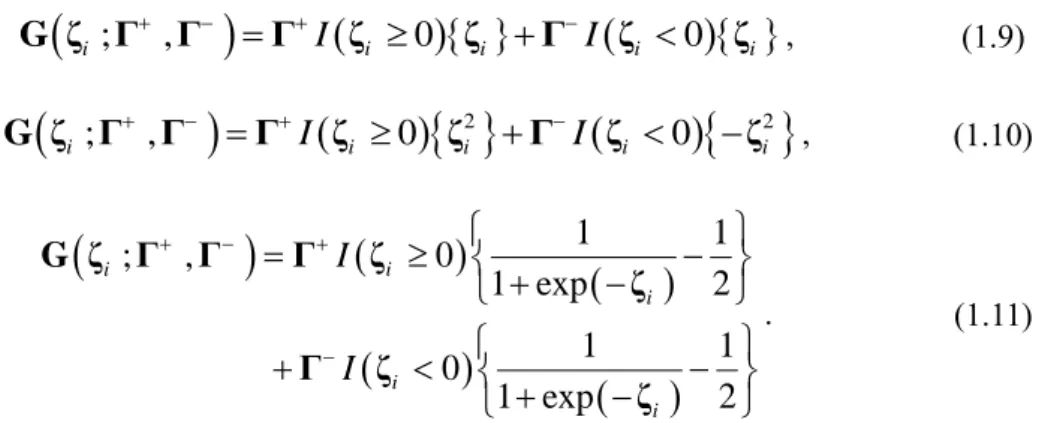
. (1.8)

The asymmetric linear model (ALM), asymmetric quadratic model (AQM), and asymmetric logistic model (ALGM) are defined as



_i

;

,



I



_i

0  

_i

I



_i

0  

_i

G ζ Γ



Γ





Γ



ζ



ζ



Γ



ζ



ζ

, (1.9)









 

2





 

2

;

,

0

i

I

i i

I

i i

G ζ Γ



Γ





Γ



ζ



ζ



Γ



ζ





ζ

, (1.10)





















1

1 ;

,

0 1 exp

2

1

0 1 exp

2

i i i i i

I

G ζ

Γ Γ

Γ

ζ

Γ

ζ

   









_



_

















_



_









. (1.11)

Table 1.1 summarizes all of the prosed models for model comparison, and Figure 1.3 shows each function described by the threshold and asymmetric models.

Table 1.1: Summary of the proposed models Figure 1.3: Proposed functions

(19)

1.4. Empirical Applications

1.4.1. Data Description

The data were gathered through a research company from two types of hotels, banks, and retail stores in Japan. The questionnaires were referred to Parasuraman et al. (1988; 1991; 1994b), and a total of 300 respondents were gathered in each service industry. Hotel B is a business hotel offering select services in low prices. Hotel A is a city hotel with some restaurants and shops located near a large station. Bank B is a local bank focusing on local customers and companies. Bank A is a megabank providing diverse services in domestic and overseas market. Retail B is a supermarket primarily selling commodities and food. Retail A is a department store with several specialty shops.

1.4.2. Model Estimation

The proposed models used the Bayesian estimation via Markov chain Monte Carlo (MCMC) algorithm with Gibbs sampling for estimation. In Gibbs sampling, conditional distributions for each random variable are considered; therefore, the algorithm of nonlinear factor analysis model is almost the same as that of the linear factor analysis model (Zhu & Lee 1999, Lee 2007), which is a major advantage of the Bayesian approach with the Gibbs sampler. However, simulating from p(𝛇𝑖| −) , 𝑝(𝜂+| −) , and 𝑝(𝜂−| −) , which are nonstandard and complex, is not an easy task.

Hence, to simulate from these distributions, the random walk Metropolis-Hastings (RW-MH) method is used within the MCMC algorithm.

1.4.3. Model Comparison

Tables 1.2 and 1.3 report that the model fits for each model were evaluated using the widely applicable information criterion (WAIC) (Watanabe 2010a, 2010b, Gelman et al. 2013) and the widely applicable Bayesian information criterion (WBIC) (Watanabe 2013). These indexes

(20)

Bayes marginal likelihood, respectively. The smaller WAIC indicates a more accurate model. The WBIC is interpreted as a minus logarithm of Bayes marginal likelihood (Watanabe 2013), so that the smaller WBIC also suggests a better model fitting.

Although the TLM is supported in Bank A and Retail B by the WAIC, the TLGM displays better WBIC for all service industries. This result also indicates that consumers’ perceived service qualities are driven by latent nonlinear structure along with the thresholds.

Table 1.2: WAIC Table 1.3: WBIC

1.4.4. Estimation Results

The Ch.1 Appendix provides the estimates of parameters in the TLGM, and Tables 1.4 and 1.5 show the estimated asymmetric and threshold parameters. Figure 1.4 describes the estimated function and distribution of unique factors for each SERVQUAL dimension.

Table 1.4: Estimated threshold parameters Table 1.5: Estimated asymmetric parameters Figure 1.4: Estimated function and uniqueness

Table 1.4 provides estimates for threshold parameters and the ranges reveal the latent zone of tolerance. This result indicates that consumers evaluate perceived service quality with an acceptable discrepancy between expectations and perceptions. The larger the positive threshold, the more difficult it is for consumers to experience service delight. In contrast, at a smaller negative threshold, consumers find it easier to tolerate service failure. When comparing the absolute value of each estimated threshold parameter in Table 1.4, the negative threshold in Hotel A, Bank B, Retail B, and Retail A are estimated to be larger than the positive threshold.

(21)

They ,therefore, obtained better results, while both thresholds mostly displayed similar estimates in Hotel B and Bank A, respectively (see also Figure 1.4). The absolute value of estimates in Bank A is the largest; thus, indicating that customers might accept discrepancies more easily in Bank A. Hotel B is required to pay more attention to service failures because of the smallest absolute value of the negative threshold.

“Delight” and “Failure” in Table 1.5 indicate the estimates for delight and failure parameters, and the standardized coefficients are shown in std.D and std.F. According to the 95% highest probability density interval (HPDI), all estimates are not 0. P{D < F} shows that of the two parameters, failure is greater than delight. Although some failure parameters are smaller than delight parameters in Hotel B, Bank A, and Retail B, whereas all failure parameters are larger than delight parameters in Hotel A, Bank B, and Retail A, which is parallel to the assumptions of value function. These results indicate that delight and failure parameters primarily follow the prospect theory, and that service failure, which is a negative discrepancy, has significantly more influence on the observed perceived service quality than service delight. Therefore, consumers’ evaluation process of perceived service quality has an asymmetric structure.

In Table 1.5, std.U indicates standardized estimated variances of each uniqueness factor for SEVQUAL dimensions that show the dependent efficacy of each SERVQUAL dimension. The precisions of the five dimensions’ qualities are presumed to be unequal because corresponding distributions look different. The distribution becomes flat if the factor’s uniqueness has a larger effect, whereas it becomes shaper with a smaller effect (see Figure 1.4). Smaller uniqueness indicates that the sub-dimension depends on the higher dimension (common factor) rather than on the uniqueness itself. On the contrary, larger uniqueness indicates that the sub-dimension has some unique features in comparison to other sub-dimensions. For example, estimates for Tangible in Hotel A (see Table 1.5) indicates that the Tangible factor is almost independent from the other factors, and has a larger effect than the baseline quality, so that it possesses larger uniqueness than

(22)

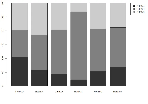
1.4.5. Segmentation for the Customer by Threshold Parameters

Figure 5 illustrates the proportion of segments for the customers in each service industry divided by the threshold parameters. P.PSQ, or the top portion of the bar plots, describes the proportion of customers whose baseline quality (second-order factor) score exceeds the positive threshold, indicating that the customers perceived positive service quality. S.PSQ, in the middle of the bar plots, indicates the class of customers whose baseline quality score is inside both positive and negative threshold parameters, whereas N.PSQ, at the bottom of the bar plots, indicates the class of customers whose baseline quality score is less than the negative threshold parameter. These plots enable the comparison of potential perceived service quality for each service industry that does not meet customer expectations.

For example, over 30 % of customers in Hotel A perceived that services exceeded expectations. Bank A achieved better service perception than other service industries; however, almost all customers might evaluate that the service is neither good nor bad because of highly proportion of S.PSQ. In Hotel B, the each segment is divided as almost equally, and the proportion of customers who perceived negative service quality is the largest among these industries, which suggests that it may be useful to improve their services.

1.5. Implications and Conclusion

Three possible implications from the proposed model are investigated and future research is discussed in this study.

First, the common nonlinear effects and independent linear effects of each SERVQUAL dimension are estimated using the second-order factor analysis with nonlinear structure. In addition, a nonlinear structure for customers’ perceived service quality is established by comparing several nonlinear measurement models. Second, a comparison of different magnitudes of effects between service delights and failures is possible by estimating the asymmetric

(23)

parameters. Third, considering the threshold parameter in the measurement model, it is possible to estimate consumers’ zone of tolerance. Moreover, the properties of the proposed model can be visualized by constructing a plot, as shown in Figure 1.4. The threshold parameters are also helpful in classifying the customers into three categories as in Figure 1.5.

In this study, the nonlinear and asymmetric measurement model with threshold is established to measure the perceived service quality. Finally, the threshold logistic model is specified, and demonstrates better results when compared with the original SERVQUAL model and the other candidate models. Moreover, using the difference score enables a proper interpretation of the threshold logistic model because both the prospect theory and zone of tolerance assume the evaluation with some reference point, such as expectation. Additional work is warranted to develop a nonparametric measurement model to explore and estimate the functional form directly. Finally, the construct validation must be extended to confirm the validity for the nonlinear measurement model, and we discuss this topic in the next chapter.

(24)

1.6. Ch.1 Figures and Tables

Figure 1.1: SERVQUAL model

Figure 1.2: Second order factor model for proposed model

(25)

(26)

(27)

(28)

(29)

Figure 1.5: Proportion of segments

Table 1.1: Summary of the proposed models

Model Nonlinearity Asymmetry Threshold Function

1_factor No No No Linear

Original No No No Linear

2nd_order No No No Linear

ALM No Yes No Linear

AQM Yes Yes No Quadratic

ALGM Yes Yes No Logistic

TLM No Yes Yes Linear

TQM Yes Yes Yes Quadratic

TLGM Yes Yes Yes Logistic

Note: 1_factor is the first-order factor analysis model with only one latent variable. Original is the SERVQUAL model proposed by Parasuraman et al. (1988), and 2nd_order is the linear second-order factor analysis model.

(30)

Table 1.2: WAIC

Table 1.3: WBIC

Table 1.4: Estimated threshold parameters

negative positive Hotel B [ -0.191 , 0.193 ] Hotel A [ -0.413 , 0.151 ] Bank B [ -0.518 , 0.193 ] Bank A [ -0.746 , 0.632 ] Retail B [ -0.427 , 0.188 ] Retail A [ -0.406 , _{0.233 ]}

original 1_factor 2nd_factor ALM AQM ALGM TLM TQM TLGM result Hotel B 15545.63 16687.35 15528.51 15515.58 15512.13 15513.99 15487.12 15528.36 15456.88 TLGM Hotel A 14341.73 15511.40 14334.90 14317.28 14322.45 14324.11 14288.40 14321.04 14281.28 TLGM Bank B 16057.84 17047.89 16041.60 16007.22 15997.80 16012.55 15971.49 16003.18 15968.51 TLGM Bank A 14261.95 15428.69 14252.64 14254.08 14227.90 14273.41 14183.03 14227.22 14197.54 TLM Retail B 15759.58 16983.10 15751.12 15741.73 15717.25 15793.99 15694.44 15721.36 15751.09 TLM Retail A 14854.60 15787.66 14848.88 14846.96 14825.10 14850.17 14801.11 14834.09 14787.83 TLGM

original 1_factor 2nd_factor ALM AQM ALGM TLM TQM TLGM result Hotel B 7402.83 8219.37 7420.27 7389.84 7380.46 7348.89 7361.30 7387.29 7331.83 TLGM Hotel A 6818.23 7666.57 6812.96 6782.97 6799.91 6752.82 6789.55 6811.24 6746.56 TLGM Bank B 7649.33 8415.56 7656.09 7618.58 7619.35 7605.23 7601.53 7615.12 7568.46 TLGM Bank A 6756.16 7587.34 6736.31 6745.13 6733.92 6701.56 6717.43 6740.27 6682.58 TLGM Retail B 7490.73 8380.04 7482.02 7475.15 7485.33 7476.88 7463.93 7478.27 7456.48 TLGM Retail A 7090.21 7796.33 7069.99 7078.22 7047.49 7016.30 7043.05 7049.40 7007.85 TLGM

(31)

Table 1.5: Estimated asymmetric parameters

Delight Failure P{D < F} std.D std.F std.U Hotel B Tangilbles←BQ 1.000 1.737 [ 1.019 , 2.438 ] 0.984 0.200 0.342 0.838 Reliability ←BQ 1.299 [ 0.790 , 1.878 ] 1.496 [ 0.975 , 2.055 ] 0.709 0.340 0.389 0.726 Resp onsiveness←BQ 2.146 [ 1.539 , 2.784 ] 2.143 [ 1.568 , 2.781 ] 0.497 0.453 0.449 0.588 Assurance←BQ 2.122 [ 1.538 , 2.781 ] 1.905 [ 1.325 , 2.469 ] 0.293 0.462 0.411 0.612 Emp athy ←BQ 2.003 [ 1.350 , 2.648 ] 1.839 [ 1.260 , 2.553 ] 0.352 0.405 0.369 0.693 Hotel A Tangilbles←BQ 1.000 1.745 [ 1.112 , 2.424 ] 0.993 0.245 0.374 0.796 Reliability←BQ 1.692 [ 1.215 , 2.206 ] 2.183 [ 1.631 , 2.726 ] 0.932 0.431 0.493 0.567 Resp onsiveness←BQ 1.987 [ 1.480 , 2.522 ] 2.818 [ 2.217 , 3.409 ] 0.993 0.435 0.547 0.508 Assurance←BQ 2.399 [ 1.740 , 3.023 ] 3.397 [ 2.704 , 4.133 ] 0.986 0.412 0.517 0.558 Emp athy ←BQ 1.835 [ 1.269 , 2.408 ] 2.648 [ 2.035 , 3.355 ] 0.981 0.376 0.481 0.622 Bank B Tangilbles←BQ 1.000 1.351 [ 0.467 , 2.212 ] 0.779 0.184 0.207 0.918 Reliability ←BQ 1.129 [ 0.542 , 1.685 ] 1.615 [ 0.988 , 2.280 ] 0.888 0.307 0.369 0.761 Resp onsiveness←BQ 1.302 [ 0.724 , 1.927 ] 2.068 [ 1.401 , 2.798 ] 0.965 0.330 0.442 0.689 Assurance←BQ 1.680 [ 1.006 , 2.409 ] 2.277 [ 1.557 , 3.072 ] 0.875 0.346 0.395 0.717 Emp athy ←BQ 1.366 [ 0.734 , 2.052 ] 2.239 [ 1.470 , 2.979 ] 0.966 0.298 0.412 0.734 Bank A Tangilbles←BQ 1.000 1.882 [ 1.141 , 2.685 ] 0.990 0.185 0.322 0.858 Reliability←BQ 1.000 1.656 [ 1.114 , 2.267 ] 0.993 0.254 0.388 0.781 Resp onsiveness←BQ 2.608 [ 1.889 , 3.328 ] 2.659 [ 1.924 , 3.445 ] 0.544 0.434 0.413 0.636 Assurance←BQ 2.979 [ 2.114 , 3.774 ] 2.915 [ 2.065 , 3.733 ] 0.447 0.436 0.399 0.646 Emp athy ←BQ 2.800 [ 1.890 , 3.604 ] 3.117 [ 2.264 , 4.061 ] 0.699 0.387 0.403 0.683 Retail B Tangilbles←BQ 1.000 1.923 [ 1.058 , 2.733 ] 0.988 0.175 0.178 0.877 Reliability ←BQ 0.953 [ 0.392 , 1.553 ] 2.052 [ 1.292 , 2.876 ] 0.991 0.201 0.210 0.794 Resp onsiveness←BQ 1.359 [ 0.854 , 1.869 ] 1.694 [ 1.159 , 2.273 ] 0.843 0.409 0.402 0.640 Assurance←BQ 1.956 [ 1.276 , 2.637 ] 2.010 [ 1.371 , 2.677 ] 0.544 0.442 0.429 0.661 Emp athy ←BQ 1.490 [ 0.890 , 2.127 ] 2.057 [ 1.318 , 2.762 ] 0.898 0.328 0.332 0.723 Retail A Tangilbles←BQ 1.000 1.499 [ 1.000 , 2.107 ] 0.970 0.282 0.383 0.769 Reliability←BQ 2.173 [ 1.530 , 2.779 ] 2.650 [ 1.951 , 3.278 ] 0.858 0.425 0.476 0.588 Resp onsiveness←BQ 1.892 [ 1.284 , 2.469 ] 2.302 [ 1.628 , 2.920 ] 0.852 0.417 0.466 0.603 Assurance←BQ 2.428 [ 1.788 , 3.123 ] 3.223 [ 2.483 , 3.987 ] 0.952 0.414 0.504 0.570 Emp athy ←BQ 1.866 [ 1.225 , 2.460 ] 2.138 [ 1.527 , 2.803 ] 0.746 0.387 0.407 0.679 95%HPDI 95%HPDI

Note 1: std.D, std.F, and std.U are standard coefficients for Delight, Failure, and Uniqueness, respectively.

Note 2: Bank A fixed two parameters to avoid improper solutions, whereas the other industries fixed only one parameter in factor loadings.

(32)

1.7. Ch.1 Appendix: MCMC Algorithm for Threshold Logistic Model

1.7.1. Details of Second-order Measurement Equation for TLGM

The second-order measurement equation in base model (1.4) can be expressed as

i

τ

)

ΓF(ζ

τ

)

G(ζ

ω

i i i i









, (1.12) where, 1 ,1 2 ,1 3 ,1 4 ,1 5 ,1 1 ,2 2 ,2 3 ,2 4 ,2 5 ,2



         





 











Γ

T _, (1.13)











f ζi



,f ζi





T        i F(ζ ) , (1.14)

 























2

1 exp

1

1 }

0 {

)

(

x

I

x

f

, (1.15) and

 























2

1 exp

1

1 }

0 {

)

(

x

I

x

f

. (1.16) 1.7.2. Prior Distribution Parameter Settings



,0 . . ,0



. ~ , | j j j j j



 N 



 H  j,0 0, H.j,0 I



, ,0 , ,0



,j ~IG  j ,  j 









,j,0 0.01,



,j,0 0.01



,0 . , ,0



. ~ , | k k k k k



 N 



 H  k,0 0, H,k,0 I



, ,0 , ,0



,k ~IG k , k 









,k,0 0.01,



,k,0 0.01   0 ,max 



0 0



| ~trN ,





 

Z Z



₀



0

,



₀



1

  min ,0



0 0



| ~trN ,





 

Z Z



₀



0

,



₀



1

(33)

1.7.3. Full Conditional Distribution [1]



 



1 , , , , , , , , . i i i i i N ε τ 1 1 T 1 T 1 1 1 T 1 τ ε ε τ τ ε ω | Λ Ψ Δ ζ Γ η η y Δ Λ Ψ Λ Λ Ψ y Δ G Δ Λ Ψ Λ                _ _ _    (1.17) [2] Λj |



,j ,Ω Y,  N



a,j ,



,jA,j



(1.18) where,



1



1 0 , , ,

A

 _j



H

_j



ΩΩ

T  and j



j



H

j

Λ

j



ΩY

j



 0 . 1 0 , , , ,

A

a

_ _ _ . [3] _,

|

_{, ,0} _,

2

j j j

n

,

IG

,

Ω Y

  

















_

_





_

_

. (1.19) where,



1 _, _.₀ _,₀ _,₀



, , 0 , , ,

a

A

a

2

1

j T j T j j j T j j T j j j 

Y

  

Λ

H



Λ













.

Set 𝑡(= 1, ⋯ , 𝑇) as a number of MCMC iterations and the RW-MH algorithm for 𝑝(𝜁𝑖|𝚪, 𝚫𝜏, 𝜎𝜁2, 𝛚𝑖, 𝜂+, 𝜂−) , 𝑝(𝜂+|𝚭, 𝚪, 𝚫𝜏, 𝜎𝜁2, 𝛀, 𝜂−) , and 𝑝(𝜂−|𝚭, 𝚪, 𝚫𝜏, 𝜎𝜁2, 𝛀, 𝜂+) are following [4]



1



,

t t i

N

i ζ

ζ





_. (1.20) The probability of accepting is









2 1 2

|

,

min

,1

|

,

t i i t i i

p

   



 



 

    

















ζ

Γ Δ

ω

ζ

Γ Δ

ω

. (1.21) [5] , _ _{ }_



, 1



0 ,max , t t k trN _Z _





    _. (1.22) [6] , _ _{ } _



, 1



min ,0 , t t trN _Z _







 



 . (1.23)

The probability of accepting is







 









 



, , 2 , 1 , , 1 , , 1 , 1 2 , , 1 , , 1

,

|

,

min

,1

,

|

,

t t t t t t t t t t t t

p

Γ Δ

Ω Z

Γ Δ

Ω Z

   









 

                 

















. (1.24)

𝜎𝜁, 𝜈𝜂+, and 𝜈_𝜂− are step-size parameters which are given so that each acceptance rate becomes

(34)

Threshold Measurement Model for Perceived Service Quality [7] k |



,k , , ,



N



a,k ,



,kA,k



   Γ Z Ω  . (1.25) where,



1 _ _, ₁_{ } _, ₁_



1 0 , , ,

A

__k



H

__k



F

_k_k_

F

T_k_k_  , and

a

__,_k



A

__,_k



H

__,1_k_,₀

Γ

_k_.₀



F

__k_,_k_₁_

Ω

_k



. [8] _,k

|

,

_{,k ,0}

,

_,k

2 n

IG

Z Ω

  











_









_

_





_

_

, (1.26) where,



1 _, _.₀ _,_,₀ _,₀



, , 0 , , ,

a

A

a

2

1

k T k T k k k T k k T k k k 

Ω

  

Γ

H



Γ













_.

The above results are valid for situations where all elements of 𝚲 and 𝚪 are free parameters. As an example, consider that 𝚲_𝑗𝑇_{and the 𝑗th row of 𝚲 contain fixed parameters. Let 𝒄}

𝑗 be the

corresponding 1 × 𝑞 row vector such that 𝑐_𝑗𝑘 = 0 if 𝜆𝑗𝑘 is a fixed parameter, and 𝑐𝑗𝑘= 1 if

𝜆𝑗𝑘 is an unknown parameter. As for 𝑗 = 1, ⋯ , 𝑝 and 𝑘 = 1, ⋯ , 𝑞, let 𝑟𝑗= 𝑐𝑗1+ ⋯ + 𝑐𝑗𝑞 be

the number of unknown parameters in 𝚲_𝑗𝑇_{, 𝚲}

𝑗∗𝑇 be a 1 × 𝑟𝑗 row vector that contains the only

unknown parameters in 𝚲_𝑗𝑇_{, and 𝛀}

𝑗∗ be a 𝑟𝑗× 𝑛 submatrix of 𝛀 such that all the rows

corresponding to 𝑐_𝑗𝑘 = 0 are deleted. Let, 𝐘𝑗∗𝑇 = (𝑦𝑗,1∗ , ⋯ , 𝑦𝑗,𝑛∗ ) with





* , , , , 1

1

q j i j i j k k i jk k

y

 

c









. (1.27)

Equation (27) subtracts the constant terms from 𝐘𝑗. Hence, the conditional distributions with 𝚲𝑗,

𝐘𝑗, and 𝛀 in part of (𝚲, 𝚿𝜖) must be replaced by 𝚲𝑗∗, 𝐘𝑗∗, and 𝛀𝑗∗, respectively. This procedure

is also adapted in full conditional distribution for (𝚪, ∆_𝜏) because 𝛾_1,1+ _{and 𝛾}

1,2+ are fixed by 1

in Bank A, and 𝛾_1,1+ _{is fixed by 1 in the other industries to avoid improper solutions. Moreover,}

𝜎𝜁2, the variance of 𝜁𝑖, is fixed by 1 to identify this model. The basic and related algorithms are

(35)

Construct Validation for a Nonlinear Measurement Model

Chapter 2 Construct Validation for a Nonlinear Measurement Model

2.1. Introduction

The psychological scale, known as the “marketing scale” in marketing and consumer behavior research, is an instrument used to measure latent psychological constructs by applying factor analysis as measurement model. Assuming some constructs for consumer psychologies and behaviors, structural equation modeling (SEM) is often used with these constructs specified by the measurement model. Before estimating by SEM, we usually evaluate reliability and validity to check the accuracy of the estimated constructs. Hence, construct validity is an important topic to estimate the causal relationship among constructs in consumer research.

Construct validation has been discussed by a number of researchers (e.g., Cronbach & Meehl 1955; Campbell & Fiske 1959; Bagozzi et al. 1991; Anderson & Gerbing 1992; Messick 1995; Hu & Bentler 1998, 1999; Edwards 2001, 2003; Malhotora & Birks 2007; MacKenzie et al. 2011; Hughes 2018), and the modern concepts have been established by Messick (1995). Because we deal with uncertain and unobserved variables, researches are concerned about reliability and validity of latent variables; from not only a theoretical but also an empirical perspective. Therefore, some statistical methods of construct validation have been discussed and developed uniquely in the marketing area (Hair et al. 2009; Bagozzi & Yi 1988; Fornel & Lacker 1981).

The measurement model and validation for the constructs have a strong relationship with classical test theory (CTT). Although most researchers have not mentioned this relationship in practical research, CTT is a very important subject in psychometrics. In addition, the relationship

(36)

between CTT and item response theory (IRT) is given Turker (1946) and Lord and Novick (1968); thus, IRT model is recognized as one kind of nonlinear CTT model in psychometrics (Lewis 2006).

In consumer research, however, CTT is always assumed implicitly when using the measurement model with questionnaires. Besides, methods related to measuring constructs have been extended with a linear CTT assumption; that is, observed scores are linearly rerated to true scores. Although this assumption makes it easier to measure true scores and to estimate reliability, it is necessary to consider the possibility of measuring error problem caused by choosing an inappropriate functional relationship between the observed and true scores.

The purpose of this study is to discuss a nonlinear measurement model and its construct validation in consumer research. First, we review the linear measurement model and the construct validation. Second, we discuss effective construct validation methods for a nonlinear measurement model. Third, the results of several simulation studies and empirical analysis using SERVQUAL (PZB 1985; 1988) are provided. Finally, we discuss the importance of construct validation and its extension to interpretable machine learning.

2.2. Linear Measurement Model and Construct Validation

2.2.1. Linear Factor Analysis Model and CTT

CTT is a traditional psychological measurement theory based on the concept of a “true score” in psychometrics (e.g., Novick 1966; Traub 1997; Jones & Thissen 2006; Lewis 2006). In the most basic approach to the measurement model of CTT, the observed score Z is considered to be the sum of a true score T and a random error E:

E T

Z   . (2.1)

The standard deviation of the errors E indicates a statement of the (rack of) precision, or standard error, of the observed score. We want to measure the true score T, but we can only obtain the observed score containing the measurement error. Because the true score can be regarded as a

(37)

latent variable, factor analysis is a standard method used to estimate the true score T, called the “construct” or “latent trait.”

There are mostly three kinds of definitions for the measurement model, depending on different parameter assumptions (Jöreskog 1971; Novick & Lewis 1967; Rajaratnam et al. 1965); see Figure 1. To explain the difference among the three measurement models with factor analysis, we define a general equation form for independent individual 𝑖 (𝑖 = 1, ⋯ , 𝑛) and for item 𝑗 (𝑗 = 1, ⋯ , 𝑝): ji i j ji t z 







, (2.2)

where 𝑧𝑗𝑖 is a observed or standardized observed variable, 𝜆𝑗 is a factor loading called the

“discrimination parameter” (or “regression coefficient”) for item 𝑗, 𝑡_𝑖 is a common factor or a latent variable corresponding to the construct as a true score, and 𝜀_𝑗𝑖 is the measurement error assumed to be distributed as a normal distribution. The assumptions of CTT are represented by (2.2) with the following equations:

 

t

_i



0 E

for all 𝑖, (2.3)

 

t

_i



1 Var

for all 𝑖, (2.4)

 

_ji  0

E



for any 𝑗 and all 𝑖, (2.5)

 

ji j

Var







for any 𝑗 and all 𝑖, (2.6)



_ji, _si



 0

Cov



for any 𝑗 ≠ 𝑠 and all 𝑖, (2.7)



ti, ji



 0

Cov



for any 𝑗 and all 𝑖. (2.8) The first, parallel measurement model is that the construct has the same degree of discrimination for each item and that the precision for each item is common. Hence, the following restrictions are additionally assumed:

p



(38)

p



₁  ₂    . (2.10)

The second, tau-equivalent measurement model, assumes that the construct has the same discrimination for each item, but that all the items have a different precision. Hence, we additionally assume restriction (2.9) and that 𝜓𝑗 for any 𝑗 is a different parameter. The third,

congeneric measurement model assumes that the construct has a different discrimination for each item and that each item has a different precision. Hence, 𝜆_𝑗 and 𝜓_𝑗 for any 𝑗 are treated as different parameters.

Therefore, each model can be estimated by factor analysis model with setting above restrictions. In marketing and most the other social science areas, congeneric measurement model is a standard method to estimate constructs.

Figure 2.1: Three different measurement equations

2.2.2. Misspecification between Reflective and Formative Models

Another kind of measurement model, the formative model, represents a principal component analysis (PCA) model specification. Although this model can be regarded as one kind of the factor analysis model from the view of probabilistic principal component analysis (PPCA), the refractive and formative model are treated as different specifications (see Figure 2) in consumer behavior research. Jarvis et al. (2003) discussed the misspecification between refractive and formative models in consumer behavior research. They investigated the top journals related to Marketing (Journal of Marketing Research, Journal of Marketing, Journal of Consumer Research, Marketing Science,) and found some studies in even those top journals contain the misspecification. Because this misspecification provides a different estimate for the parameters in the structure model, it is important to clarify the assumptions between observable and latent variables when applying the measurement model.

(39)

Figure 2.2: Reflective and formative models

2.2.3. Linear Factor Analysis Model and Construct Validation

This section introduces different kinds of reliability coefficients and a method to evaluate the convergent and discriminant validity for construct validation.

2.2.3.1. Measurement Model and Reliability Coefficient

Reliability in CTT is defined as the proportion of observed score variance due to variance among individual true scores (Novic 1966; Lewis 2006; Webb et al. 2006). Coefficient alpha or Cronbach’s alpha (Cronbach 1951) is most frequently used in the present methods (MacKenzie et al. 2011). From the composite measurement (Novic & Lewis 1967) aspect, we can obtain another expression of Cronbach’s alpha in Eq. (2.11) and Ch.2 Appendix A.1, and it is helpful to understand the relationship between the measurement model and the reliability coefficient. Equation (2.3) indicates that Cronbach’s alpha represents a reliability coefficient when assuming the tau-equivalent test. In other words, this reliability estimates a coefficient to evaluating a measurement model with the condition that the factor ladings are equal for all observed variables. Therefore, when standard factor analysis is assumed, Cronbach’s alpha is not suitable to evaluate the reliability for the measurements:

 

2 2 1 2 2 1

1

p ji j t p j j

Var z

p

Var Z

_p









 





















_







. (2.11)

Another well-known estimator for reliability is coefficient omega (McDonald 1978). As in the case of coefficient alpha (see Ch.2 Appendix A.2), coefficient omega can be expressed as Eq. (2.12). This is a reasonable estimator for the reliability of a congeneric test, which is a standard assumption of factor analysis. Moreover, the third entity in (12) was proposed for construct

(40)

MacKenzie et al. 2011). This estimator is also valid for the parallel and tau-equivalent tests so that coefficient omega (or CR) is a generalization of the reliability estimator among the three basic test models:

 

_



_



2 1 1 2 1 1

1

p p j j j j t p p j j j j

Var Z











   

 







. (2.12)

2.2.3.2. Convergent and Discriminant Validity

Convergent validity is a confirmation that measures for the same construct have adequate relationships with each other, and the measures should be distinguished from that for other constructs. This is called “discriminant validity.” Both validations are required for justification of a novel trait measure, validation of test interpretation and establishing construct validity (Campbell and Fiske 1959). Campbell and Fiske (1959) proposed multi trait method matrix (MTMM) to evaluate convergent and discriminant validity jointly. However, it is inconvenient for secondary users to prepare additional different measurement methods. Moreover, Bagozzi et al. (1991) showed that MTMM is not effective in several situations because of the limited assumptions.

Confirmatory factor analysis (CFA) also provides a method for convergent and discriminant validation (Anderson & Gerbing 1988; Bagozzi & Yi 1988 Bagozzi & Phillips 1982). In most situations, applying CFA results is useful to check construct validity. However, comparison between the fixed correlation (equal to 1) and the unfixed CFA models for discriminant validity is not effective because high correlation (equal to 0.9) can still produce significant differences in fit between the two models (Hair et al. 2009).

For effective judgment, average variance extracted (AVE), which was also produced by Fornell & Larcker (1981), can be applied to evaluate both convergent and discriminant validity (Fornell & Larcker 1981; Hair et al. 2009; MacKenzie et al. 2011). AVE is defined as Eq. (2.13)

東北大学機関リポジトリTOUR

Extending Construct Measurement and Validation

in Marketing and Consumer Behavior Research: A

Study of Nonlinear Measurement Model and

Interpretable Neural Network

著者

佐藤 平国

学位授与機関

Tohoku University

学位授与番号

11301甲第18997号

Extending Construct Measurement and Validation in Marketing

and Consumer Behavior Research: A Study of Nonlinear

Measurement Model and Interpretable Neural Network

Toshikuni Sato

Graduate School of

Economics and Management

Tohoku University

Contents

Preface

Acknowledgments

Introduction

Chapter 1

Threshold Measurement Model for Perceived Service Quality

1.1. Introduction

1.2. Related Literature

1.3. Model Development



 



Λω

ε

y





 

G

ζ

τ

ω





 





 

Λ

G

ζ

τ

ε

ΛG

ζ

Λτ

ε

y

































1

1

;

,

,

,

0

2

佐藤平国

_

_

_

_

_

_

_

_