JAIST Repository https://dspace.jaist.ac.jp/

(1)

JAIST Repository

https://dspace.jaist.ac.jp/

Title コンピュータグラフィックスにおける媒体中の剛体運

動シミュレーション

Author(s) 謝, 浩然

Citation

Issue Date 2015‑03

Type Thesis or Dissertation Text version ETD

URL http://hdl.handle.net/10119/12755 Rights

Description Supervisor:宮田一乘, 知識科学研究科, 博士

(2)

Doctoral Dissertation

Immersed Rigid Body Dynamics in Computer Graphics

Haoran Xie

Supervisor: Professor Kazunori Miyata

School of Knowledge Science

Japan Advanced Institute of Science and Technology

March 2015

(3)

Keywords: real-time, immersed rigid body, free fall, phased diagram, turbulent ﬂow, data-driven simulation, two-way coupling, aerodynamics, unsteady dynamics, model reduction, motion synthesis, motion patterns, precomputation, computer graphics

(4)

Be not immortal, since it is flame.

Be infinite, while it lasts.

— Sonnet of Fidelity, Vinicius de Moraes

(5)

Abstract

The real world is complex and specular: a leaf falling down from a tree side byside, a coin moving underwater swaying left and right, and the falling snowflakes dancing up and down in even still flow environments. Unfortu- nately, the virtual worlds under the conventional animation techniques utilize the ideal models with no consideration of the detailed effects of the flow environments, which take account of the inertial, viscous, and turbulent features in high Reynolds number flow. Although the physical simulations have dramatic success in 3D films, games and virtual reality applications in recent decades, the simulations of unsteady and turbulent dynamics frustrate researchers in both computation cost and simulation fidelity.

To solve these issues, this dissertation proposes a new topic,immersed rigid body dynamics, into the real-time computer graphics community. It is clearly different from the other traditional topics in computer graphics that the research aim of immersed rigid body dynamics is to simulate the motion of rigid body fully immersed or submerged inside real flows, and strongly coupled with the surrounding flows. This dissertation presents a family of algorithms for real-time simulations of immersed rigid body dynamics in computer animation.

These algorithms are built on data-driven simulation methods to simulate the rigid body dynamics with the flow effects in computer environment. These approaches make it feasible to achieve realistic simulation results in low computation cost. In addition, a promising prior reduced model of dynamical systems is introduced for the parameter identification into computer animation.

The first contribution is a graph-based framework for synthesizing the motions of immersed rigid body, which are commonly lightweight. This framework is a first try to combine the motion graph technique in character animation field with the physics-based simulations. The typical motion patterns of immersed rigid-body dynamics are extracted in a phase diagram and verified from thousands of physical experiments to construct a precomputed trajectory database and the transition probabilities in Markov-chain model of the motion graph.

Finally, an improved noise-based algorithm is proposed for integrating the wind ﬁeld with the simulation results.

(6)

The second contribution is a stochastic model of immersed rigid body dynamics. This model first utilizes energy transport model of the surrounding turbulent flow to approximate the energy distributions due to the rigid body motions. Then, the proposed turbulent model is successfully introduced into a generalized Kirchhoff representation of the rigid body dynamics with Langevin model in a stochastic Wiener process. The proposed model adopts a new approach combining the precomputed simulation data of turbulent energy and the runtime simulations of rigid body solvers.

The third contribution focuses on a pattern-driven framework for immersed rigid body dynamics. This simulation framework first classifies the influences of parameter spaces of viscous force coefficients in a data training process, and then proposes a curvature-based motion planning method to represent the unsteady dynamics due to the vortex shedding. The proposed methods learns the knowledge of parameter subspaces of the rigid body dynamics from numerical experiments in a new dynamical model, which clarifies the viscous forces from the surrounding flow into three components and reveals the relationships among the force coefficients, the Reynolds number, and angle of attack of the body. In addition, the proposed framework combines the motion graph technique from the graph-based framework and the energy optimization in motion synthesis from the stochastic model.

Finally, a novel reduced model of dynamical systems is constructed, which can accelerate the parameter estimation of physical parameters in a dynamical model with low computation cost. In contrast to the conventional reduced order models, the proposed model is a prior meta-model of dynamical systems based on the separated representation in large domains including initial conditions, boundary conditions, and physical parameters. The proposed model does not depend on the preprocessed snapshots of the solutions from dynamics solvers.

This model is successfully applied to the weakly coupled and nonlinear problems. The improvement of the proposed reduced model in strongly nonlinear problem, such as immersed rigid body dynamics, is worth being anticipated.

(7)

Acknowledgments

As I am finally summarizing this dissertation, I would like to thank and ac- knowledge many people for their support, help and encouragement over the years enrolling in the five-year-program of JAIST, Ishikawa, Japan, which is the most wonderful institute hovering in the blue sky over the mountains of imagination and innovation. First and foremost, my sincere thanks to my advisor, Prof. Kazunori Miyata for his vision and inspiration to visual simulations in computer graphics, for his guidance and commitment to pursue researches on persistence and think topics profoundly, and for his generosity of various research opportunities and encouragement to the qualified thinking of the challenging simulation problems.

During my graduate studies, it is great luck to have the chances to meet and discuss with excellent researchers in different research fields, including but not limited to computational fluid dynamics, computer vision, software engineering, complexity science, and computer graphics. Thanks to my great advisor and the sophisticated education system, I have been enjoyed three internship opportunities in the University of Sydney (2011), University of California (2012) and Kent state university (2013). I would like to thank all the friends among the internships who help me accommodate the cheerful life overseas.

I am also grateful to the members of my thesis committee: Prof. Kazunori Miyata, Prof. Taketoshi Yoshida, Prof. Huynh Nam Van, Prof. Ho Bao Tu in JAIST and Prof. Shigeo Morishima from Waseda university. Their professional suggestions and feedbacks help me to improve this dissertation greatly. I would also thank Dr. Ye Zhao, the advisor in Kent state university for conducting my minor research, and Prof. Takashi Hashimoto for his great inspiration on research problems, and Prof. Norishige Chiba for his constructive discussion on my research topic in the short visit to the computer graphics lab of Iwate university.

In addition, I would like to thank all the members in Miyata laboratory, especially, Mr. Xiaodong Du for accommodating my early life in Japan, and Dr. Ken Ishibashi for sharing his great research experiences and his help on the application of research fellow of Japan Society for the Promotion of Science, and Dr. Thao Ngoc Nguyen for her helpful discussions on computer vision problems.

Finally, I have been deeply indebted to my parents and elder brother for their unconditional support and encouragement.

(8)

List of Figures

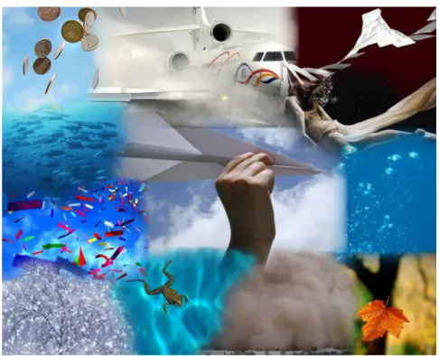
1.1 Examples of natural phenomena of the immersed bodies. Sources: Google image search. . . 3 1.2 Functional modules deﬁned in this thesis. . . 6 1.3 A family of algorithms proposed in this thesis for simulating immersed rigid

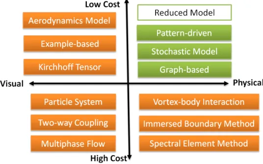
body dynamics (Green color: the proposed methods; orange color: examples of the related methods). The abscissa denotes the simulation quality, and the ordinate represents the computation cost. The details of the related work are described in the next chapter. . . 9 3.1 Six motion patterns are abstracted from experimental works [APW05b,

ZCL11], from left to right: steady decent, tumbling, ﬂuttering, chaotic, helix and spiral motions. . . 23 3.2 Overview of graph-based immersed rigid body dynamics. . . 24 3.3 The Re-I^∗ phase diagram of immersed rigid body motions from [WHH64,

SDG69, FKMN97, ZCL11], including six regimes:(a) steady descent, (b) tumbling, (c) chaotic, (d) ﬂuttering, (e) helix, and (f) spiral motions. The symbols in the diagram represent experimental results from previous works. 25 3.4 (a) Fluttering trajectory determined by solving the ODEs in Equation(3.4)

with A_⊥ = 4.1, A_∥ = 0.9 (b) Useless trajectory by solving the ODEs in Equation(3.4) with A_⊥= 4.6, A_∥ = 0.15. . . 27 3.5 Trajectory segments obtained from Equation (3.6). . . 28 3.6 Comparing synthesized trajectory (red) and measured data (black) of ﬂut-

tering motion, for no orientation (left) and interpolated orientations (right).

Arrow lines represent feature vectors. . . 28 3.7 The ﬁrst two levels of a small trajectory search tree (1) and the tree struc-

tures of ﬂuttering (2), chaotic (3), and tumbling motions(4) created by traversal of four levels of the search tree. (gl: glide left; gr: glide right) . . 29 3.8 Measured curves projected onto theXY plane: (1) steady descent motion;

(2) ﬂuttering& chaotic& tumbling motions; (3) spiral motion; and (4) helix motion. . . 30 3.9 (a) Motion classiﬁcations (blue: motion classes; green: motion groups;

Brown: motion segments). (b) Motion classes observed in experiments. . . 31 3.10 Markov chain model states and transition probabilities. . . 33 3.11 Free fall motion graph. A motion path represents a collection of splices

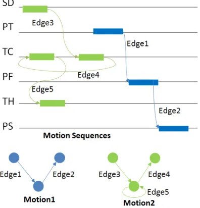
between sequences. Here, two example motions are shown. . . 34

(13)

3.12 Two-dimensional wind field, HEIGHT represents the distance (m) above the ground. The color represents the velocity length compared to the mean wind velocity U(red: V > 2U; pink: U < V ≤ 2U; blue: U/2 < V ≤ U; black: V ≤U/2), the wind direction is along the x-axis. . . . 35 3.13 Trajectory of freely falling behaviour in wind field . . . 37 3.14 Motion paths for different values of the mean wind velocity U: (a) U = 1.0

m/s,(b) U = 3.0 m/s, (c) U = 5.0) m/s. The wind direction is from right to left. . . 38 3.15 Comparison of the simulation with the ground truths of one-Japanese yen

coin falling motion in water. . . 39 3.16 Comparison of the simulation with the ground truth of a paper falling mo-

tion in air. The ﬁgure of the ground truth is blurry because of the dim background in each frame of the captured video. . . 40 3.17 (a) Comparison of the simulation with the ground truth of a leaf falling

motion in air. The simulation of the motion in a wind ﬁeld of mean wind velocity U = 3.0 m/s (b) and U = 5.0 m/s (c). The wind direction is from right to left in a screen space. . . 41 3.18 Simulation of multiple leaves falling from a tree. . . 42 4.1 Overview of the proposed stochastic model. The steps in grey color run in

precomputation steps. The runtime includes only two steps in blue color so that the computation cost is signiﬁcantly reduced. . . 45 4.2 Turbulent parameters (χ, ε) in time steps withRe= 3.8×10³and 32×32×16

MAC grids. . . 51 4.3 Simulation results of a piece of paper falling in air. (a) initial release angle

= 75^◦; (b) initial release angle = 30^◦. . . 54 4.4 Comparison between the simulation and the ground truth of a ﬂying paper

airplane. . . 55 4.5 Comparison among (a) ground truth,(b) previous work and (c) the proposed

approach. Ground truth shows oscillations generated in diﬀerent directions (the shorter silhouettes manifest the oscillation in three dimensions.), previous work takes account only Kirchhoﬀ tensor, whereas the proposed model has concerned the vortical loads. . . 56 5.1 The proposed pattern-driven framework consists of a dynamical model, data

training of motion patterns, and motion synthesis of immersed rigid body dynamics. . . 59 5.2 Computation errors between previous approach and the analytic solution

for diﬀerent bodies. For both cases , the relative error becomes larger with smaller thickness. The previous approach fails (error > 1.0%) when the thickness is smaller than 1.3 cm for ellipsoid and cylinder structures. . . 62

(14)

5.3 The illustration of the drag, rotational lift, and translational lift forces in body-fixed frame, which are corresponding with the translational velocity (blue) and angular velocity (yellow) and their cross products in the left subfigure. . . 64 5.4 Drag and lift coefficients related to the angle of attack. The dashed lines rep-

resent the lift coefficients and the solid lines for drag coefficients by the proposed parameter model. The circle-marked data [JWL⁺13] is fitted by Data 1 (C_D = 0.26, C_L1 = 2.98, C_L2 = 0.59); the square-marked data [WP03]

by Data 2 (C_D = 2.0, C_L1 = 1.02, C_L2 = 0.70); the triangle-marked data [OFM09] by Data 3 (C_D = 2.70, C_L1 = 1.31, C_L2 = 0) in the proposed model. 65 5.5 Comparison between the simulation result of the proposed dynamical model

(rectangle area in the left subﬁgure) and the captured trajectory from [VCW13]

in right-top subﬁgure. . . 66 5.6 Four motion patterns of a falling card from rest observed in this work,

where the release angle is 10^◦, a = 3.5cm, and b = 2cm: (a) SD (˜c = (1.81,0.31,0.31)); (b) AZ (˜c= (0.61,1.81,1.21)); (c) ZZ (˜c= (0.31,0.91,0.61));

(d) AR (˜c= (0.61,2.71,0.91)). The unit of the spacial coordinates is cm. . 68 5.7 The distinction among four motion patterns. SD (red points, left-top subﬁg-

ure): (d= 1.25, e= 0.72); ZZ (green points): (d= 5.69, e= 0.79); AZ (blue points): (d = 13.72, e= 0.93); AR (magenta points): (d= 22.43, e = 0.92).

The projected points are corresponding to the trajectories in Figure 5.6 with the same colors. For better appearance, the points of AZ and ZZ are rotated in π/2 and π, respectively. . . . 70 5.8 Clustering results of falling card and falling leaf motions. The diﬀerent

colors represent diﬀerent motion patterns. red: SD; green: ZZ; blue: AZ;

magenta: AR. . . 71 5.9 Sampling process from low resolution to high resolution sampling. (a) 2D

illustration. The red and green colors denote different patterns. In the middle figure, the data (+) represent the new sampled data, and the black triangles represent the data on the boundary to be resimulated. (b) The boundaries among parameter subspaces after resampling. . . 72 5.10 Parameter subspaces of different motion patterns of falling card motions.

Red: SD; green: ZZ; blue: AZ; magenta: AR. . . 73 5.11 Motion transitions among motion patterns. . . 74 5.12 Curvature curves corresponding to the motion patterns in Figure 5.6 (Red:

SD; green: ZZ; blue: AZ; magenta: AR). The square points on the motion curves denote the maximum values detected on the curvature curves with a tolerance 0.1. For better appearance, the curvature values of ZZ, AZ, and AR are added by 0.2, 0.4, and 0.6, respectively. . . 76

(15)

5.13 Simulation results with different flow effects: (a) rigid body solver without flow effects; (b) rigid body solver with inertial effect (previous method);

(c) rigid body solver with inertial effect (proposed method); (d) rigid body solver with inertial effect (proposed method) and viscous effect (previous method); (e) proposed dynamical model with both effects; and (f) proposed immersed rigid body solver with inertial, viscous, and turbulent effects. . 78 5.14 Comparison of simulation results and ground truth of a leaf falling in air:

(a) ground truth from captured video; (b) optimized control parameters in parameter subspaces (SD, red; AR, magenta). All grid surfaces denote boundary surfaces among parameter subspaces. . . 79 5.15 Force coeﬃcients C_d, C_l1 and C_l2 of drag, rotational lift, and translational

lift forces, respectively. . . 80 5.16 Comparison between diﬀerent simulation results of leaves falling from a tree

in air under the same initial conditions and the ground truth (top-left sub- ﬁgure). . . 81 6.1 Illustration of the separated representation. . . 85 6.2 (a) Numerical result of the separated representation. (b) Computation error

compared with the reference solution. . . 89 6.3 First six functions of T_i(t) and K_i(k). (Note that the values of functions

have been curve ﬁtted by the polynomial curves) . . . 90 6.4 Simulation result and its error compared with exact solution. The parame-

ters are ρ_f = 1.23, g = 9.81, A= 0.5, m= 0.1. . . 91 6.5 Convergence of our approach toward the exact solution as iteration increased. 91 6.6 Comparison with reference results for diﬀerent values of initial conditions

(lines represent reference results; empty squares represent the computation results of our separated representation (red: u₁; blue: u₂; green: u₃)) . . . 93 6.7 (a) Convergence of simulation results after iterations in the coupled model

with initial conditions corresponding to the case of Figure 3 (d). (b) Com- putation times compared with a simple iterative procedure. . . 94 6.8 (a) Simulation result with initial velocities [1.0,1.0,1.0,1.0,1.0,1.0] and (b)

its computation error (red: translational velocity; green: angular velocity) . 94 6.9 Weighted combination of linearized model at expansion pointsx1, x2, x3 and

x₄ in a 2D state space. The range of the blue circles present the valid ranges around expansion points. LineAdenote the sampling points from a training input. Note that lineB andCcan be approximated well because they locate inside the weighted regions. In the contrary, red line D is badly represented. 97 7.1 Global review from the view of knowledge science. The functional modules

are corresponding to the explanations in Section 1.3.1. . . 101 7.2 Perceptual knowledge of immersed rigid body dynamics. . . 103 7.3 Evaluations of the simulations results by the proposed approaches. G1, G2,

G3, S4, S5, S6, P7, and P8 are corresponding to the simulation results in Figures 3.15, 3.16, 3.17, 4.4, 4.5, 5.5, 5.14, and 5.16, respectively. . . 104

(16)

List of Tables

1.1 Combinations of diﬀerent modules in all proposed methods. . . 8

2.1 Summary of previous investigations on immersed rigid body dynamics from physical experiments in the order of published years. . . 12

2.2 Summary of previous investigations on immersed rigid body dynamics from numerical experiments in the order of published years. . . 16

4.1 Notation used through this chapter (Bold letters denote vector variables.). 47 4.2 Computation cost of the simulation results on runtime. . . 56

5.1 Summary of control parameters in previous experimental work. . . 67

5.2 The conﬁgurations of all the simulations in our implementations. . . 77

7.1 Comparisons of proposed methods in diﬀerent criteria. . . 101

(17)

(18)

Chapter 1 Introduction

Since Dr. Ivan Sutherland invented the computer drawing system Sketchpad in 1962, computer graphics has been improved profoundly into various topics, including computational geometry and modelling, shading and rendering, animations and simulations. When time comes to the year of 1999, there are two important events playing significant roles in physical simulations to twenty-first century: NVIDIA created the world first graphics processing unit (GPU), and Jos Stam has published his famous paper ”stable fluids”, which has at- tracted around 1,500 citations until now. The traditional physical simulation in computer graphics includes the rigid body simulations, deformable simulations, and fluid simulations.

The developments of GPU and semi-Lagrangian algorithm has ignited the enthusiasm of fluid simulations and the topics in other physical simulations. The researcher started to try more challenging topics, such as two-way coupling among fluids and bodies, turbulent flow, multiphase flow, and so on. The successful computer graphics techniques make the 3D films and games become popular to attract people worldwide. The applications of virtual reality make users immersed in a virtual world that has never happened before.

Even with the help of GPU computations, the simulation work always pursues a better trade-off between computation cost and simulation fidelity. The real-time simulations are urged in various applications, such as online games, mobile games, surgical simulations, and animation design systems, where an interactive system allows the computer to provide instantaneous feedback to the user’s operations. Note that the physical simulations usually refer the simulations of physics-based dynamical systems, such as the visual simulations of natural phenomena and different bodies, e.g., rigid and soft bodies and particles [Par12].

There is another important ﬁeld in computer animation, character animation, which covers various topics as human motion, facial animation, hand animation, and so on. Although it seems that the techniques of physical simulations and character animations are quite diﬀerent, this thesis has a successful try to introduce the character animation technique into physical simulations with motion styles by a motion graph. The pursuit of both

(19)

realistic and real-time simulations facilitates researchers to develop new algorithms, so that the state-of-art physical simulations in computer graphics have two main categories:

physics-based methods and data-driven methods. All the proposed approaches in this thesis belong to data-driven simulations to achieve realistic simulations in low computation cost. The data-driven methods are specially useful to simulate complex dynamics in two ways: capturing the complex behaviours using data model and precomputating the heavy simulations in oﬄine processes.

The physical simulations of the complex dynamical systems are greatly challenging and promising to enhance the realness of computer animations that cannot be achieved before. The complex systems arise from high degrees of freedom (DOFs) as particles and articulated bodies, high Reynolds numbers as turbulent flows, and nonsmooth dynamics as frictional contacts of cloths and rigid bodies in computer graphics. The main purpose of this thesis is to simulate the complex systems due to unsteady dynamics with high Reynolds numbers flow as turbulent flows, and to introduce a novel topic, immersed rigid body dynamics, into computer graphics.

1.1 A novel topic

The natural phenomena of the immersed bodies around us are prevalent in daily-life.

The dynamics of an immersed body means that the motion of a body moving inside the flows, immersed in air or submerged underwater, is very sensitive affected by the surrounding flow. Precisely speaking, the immersed body undergoes the wake-induced path-instability in a strongly coupled process of vortex-structure coupling within high Reynolds number. As shown in Figure 1.1, these phenomena cover the motions of falling card, falling leaf, rising bubble, falling object underwater, swaying cloth, flying paper- airplane, snowflakes, dust, the swimming motions, and so on. In this thesis, we focuses on the fundamental immersed rigid body dynamics, and the simulation techniques of immersed rigid body can be extended to linked rigid bodies, spring-mass cloth, and particle systems straightforwardly. In contrast to the previous work in computer animation, the simulation of immersed rigid body dynamics is indicated as a novel topic in the following reasons:

• Rigid body simulations: The conventional rigid body solvers do not consider any flow effect from the surrounding flow that we can notice that a falling leaf would move downward vertically by current physics engines. The rigid body follows the classic Newton’s law like in a vacuum environment, and it is obviously inconsistent with our daily experiences,

• Two-way coupling: The coupling motions among body and ﬂuids have been studied extensively in computer graphics, there are two essential diﬀerences hindering

(20)

Figure 1.1: Examples of natural phenomena of the immersed bodies. Sources: Google image search.

the two-way coupling techniques to simulate the immersed rigid body successfully.

First, they have different physics principles, the coupling motions are usually in low Reynolds number where the turbulent effect is out of account. Then, they have different research aims: the coupling simulations mainly focus on the fluid motions, such as splashing; while the simulations of immersed rigid body focus on the dynamical states of the rigid body. Due to the immersed nature, we cannot perceive the apparent movements of the surrounding air and water so that it is inadvisable to simulate the particles’ motions for graphical applications, which are commonly in high computational costs.

• Aerodynamics simulations. The aerodynamics/hydrodynamics simulations usually utilize the approximations of drag and lift forces based on a quasi-steady as- sumption, such as the quadratic viscous forces from Kutta-Joukowski theory. In such approximations, the forces’ coefficients play a significant role in the whole process of the aerodynamics simulations, which are usually designated to be as constants, functions of angle of attack or the Reynolds number. In the situation of an immersed rigid body, it is known that the force coefficients are instantaneously changed as a complex and unknown function of angle of attack, the Reynolds of number, the body geometry and the vortex-shedding periods. In this sense, the approximations of vis-

(21)

cous forces are not suﬃcient to achieve realistic simulation results for the proposed topic.

• Multiphase flow: In computer animation, the multiphase flow simulations involve the simulations of bubble flow, dust simulations, snowfall simulations, leaves simulation, and so on. The participated bodies have different physical properties (e.g., density) from the surrounding flow particles. In these simulations, the immersed bodies are considered as sphere particles with 3 DOFs, where the non-spherical particle motions is still an absent issue which presents the same motion patterns with the proposed topic.

This novel topic is also related to the turbulent/ﬂuid simulations and character animations.

More details about the related previous work are described in next chapter. Finally, the techniques for simulating the immersed rigid body dynamics in computer graphics have to overcome the following issues: (1) The computation of coupling motions with fluid in small grids is too heavy for real-time graphical applications, (2) While simulating flow in high resolutions, the turbulent motions and their numerical dissipations are difficult to be analysed; (3) In order to achieve stable simulation results, the implementation involving boundary conditions requires infinitesimal timesteps; (4) The coupling problem among the translational and rotational velocities of the rigid body exists due to six DOFs states.

Therefore, the simulation of immersed rigid body dynamics is a challenging topic in both ﬂuid mechanics and computer graphics.

1.2 A challenging topic

This section explains why the proposed topic is considered to be challenging from the view of ﬂuid mechanics.

• Strongly coupling: Coupling between a rigid body and the surrounding flow is an important subject in computer animation based on various disciplines of engineering and physical problems. Nevertheless, the community lacks of the computation technique that can simulate a strongly coupling problem of the moving boundary with unsteady flow due to its computationally challenging and expensive issues. In contrast to the enormous literature of the rigid body dynamics, particle dynamics and two-way coupling simulations, the strongly coupled fluid-body interactions involve the vortex shedding and flow instability. To make it clear, T_f and T_r present the characteristic timescales of fluid motion and rigid body motion, respectively. If T_f ≫ T_r, then the rate of change of the surrounding flow can be neglected in comparison with the rate of change of the body, for example, a cup falling onto ground.

IfT_f ≪T_r, instead of solving a coupling dynamics, the quasi-steady approximations

(22)

of drag and lift forces using force coefficients are adequate, which are the simplified representation of aerodynamics widely adopted in wind simulations. For a strongly coupled interaction,T_f ≈T_r, the steady dynamics based on quasi-steady approximations becomes invalid anymore. The numerical difficulty arises from the nonlinearity and unsteadiness of the coupled motions due to the generation and detachment of vortices from body’s edge.

• Wake instability: The Reynolds number is a critical parameter to present the flow patterns with different dynamical similarities, and is a measurement of the relative importance of inertial and viscous effects from the surrounding flow. Re = U L/ν, whereU is the mean relative velocity of the body to the flow,L is the characteristic dimension of the rigid body, and ν is the kinematic viscosity of the flow. For low Reynolds number flow, the inertia of the flow is not important and the flow is smooth and straight forward; For higher Reynolds number, inertia begins to play an important role and vortices are generated behind the object. When the Reynolds number increases, the flow becomes unsteady from the steady state and undergoes several bifurcations. The first bifurcation leads the steady flow with low Reynolds number lose its axisymmetry at a critical number Re_c1 (Re_c1 = 212 for sphere [ERFM12], Re_c1 = 105 for disk [ZLS⁺13]). The flow motion bifurcates into two branches in planar plane of the body center line. The second bifurcation occurs atRe_c2 (Re_c2 = 273 for sphere,Re_c2 = 160 for disk) where the periodic hairpin-like vortices are shed from the symmetry plane of the body. The wake structures have the alternating sign and different magnitudes. And then, the third bifurcation occurs at Re_c3 (Re_c3 = 355 for sphere, Re_c3 = 200 for disk) where the wake becomes irregular and chaotic, and the vortex shedding makes the motion be fully in three dimensional state. As the Reynolds number increases further, the secondary vortices and the counter-rotating vortex pair are observed at the leading-edge of the rigid body.

• Path instability: The effects of wake instability are related to the oscillations of the immersed body, which invoke the motion transitions among different motion patterns of the immersed rigid body. Besides of the viscous effects with the Reynolds number, the inertial effects due to the density ratio and the body geometry (aspect ratio) also play a important role for the three dimensional motion trajectories. For low Reynolds number flow, the body generates small horizontal oscillations due to the vortex shedding as Karman vortex street. While the Reynolds number increases, large amplitude oscillations were found [HW10]. The observed path could change largely with the environment noise at higher Reynolds number. When the viscous effects become predominant, the body moves side-by-side along a rectilinear path; when the inertial effects become predominant, the body falls in a planar plane. As density-ratio

(23)

increases, a zigzagging motion starts and then transfers to an autorotation motion.

There are also some three dimensional motion paths observed, such as spiral and helical motions [ZCL11].

1.3 Global overview

This section describes the functional modules of this thesis in a global overview, which are adopted in diﬀerent combinations for the proposed methods to simulate immersed rigid body dynamics. To clarify the functions of each module, we deﬁne the input and output of each module to construct data-driven methods.

Figure 1.2: Functional modules deﬁned in this thesis.

1.3.1 Functional modules

As illustrated in Figure 1.2, six functional modules are deﬁned as follows.

Dynamical models provide the kinematic and dynamical equations of the states of the immersed rigid body. The states include the information about position, orientation, translational and angular velocities of the rigid body. The dynamical equations are

(24)

commonly the ordinary diﬀerential equations which can be solved by traditional Runge-Kutta (RK) method. In contrast to RK method, the variational geometric integrator based on SE(3) [KCD09] is preferred for achieve stable numerical results.

The dynamical model is designed in a generalized Kirchhoff model considering both viscous effect and inertial effect of the surrounding flow. For the purpose of motion synthesis, a dynamical model could create various motion segments to be stored in a trajectory database.

Physics experiments capture the motions of rigid bodies by high-speed cameras in the experiments of falling objects with diﬀerent geometries and densities in air or water.

In contrast to the motion capture of the body’s state at each frame, this thesis proposes a high-level capturing system of motion patterns. In terms of the captured motions, the transition matrix among motion patterns can be obtained as discrete Markov-chain model for a motion graph in motion synthesis.

Numerical experiments obtain the precomputed simulation data by tuning control parameters. Although the control parameters are defined as drag and lift forces coefficients in this thesis, the other parameters can be added properly according to the simulation purposes, such as aspect-ratio, density, and release angle of the rigid body. All the motion trajectories are classified into different motion patterns as observed in the physical experiments. Finally, the database of parameter subspaces are constructed corresponding to each motion pattern.

Motion synthesis provides a motion planning process to connect the data of different motion patterns by a motion graph. This process can be executed in runtime for the purpose of online simulations or in precomputation for storing the instantaneous force coefficients as codebook. In addition, an energy optimization is proposed to reflect the turbulent features of energy dissipation in the surrounding flow.

Real flow defines the flow effects from the surrounding flow by considering both the potential flow and the vortex flow. For potential flow, a panel method or boundary element method can be utilized to obtain the added mass tensors. For vortex flow, there are various turbulent models, such as energy transport model, Reynolds aver- aged Navier-Stokes simulation, and large eddy simulation. In this thesis, the energy transport model is used by combining with a Langevin model. The Langevin model is a stochastic process with randomness sources including white noise or colored noises.

To reduce the runtime computation cost, the turbulent model can be simulated oﬄine with the turbulent energy database as output.

Reduced model represents the coherent features of a dynamical system. In this thesis, a prior reduced model of separated representation is proposed that does not depend

(25)

on the precomputed simulation data. The computation process of reduced model can be executed in pre-computation steps.

1.3.2 Data-driven methods

All the proposed methods are data-driven simulation methods in this dissertation to achieve real time simulations. As shown in Table 1.1, the distinctions among the proposed methods are designed as follows:

Table 1.1: Combinations of diﬀerent modules in all proposed methods.

Modules Graph-based Stochastic model Pattern Driven Reduced model

Dynamical models √ √ √ √

Physics experiments √ √

Numerical experiments √

Motion synthesis √ √

Real ﬂow √ √

Reduced model √

Graph-based method utilizes a simpliﬁeddynamical model of immersed rigid dynamics to model each motion pattern from physical experiments, and synthesize the rigid body motions from the precomputed trajectory database inmotion synthesis.

Stochastic model combines the dynamical model of immersed rigid body dynamics with a Langevin model in real flow using the precomputed turbulent energy database.

Pattern Driven method adopts a motion graph with the data of motion patterns from physical experiments, and an energy optimization in parameter subspaces from nu- merical experiments of a proposed dynamical model, which is combined with the turbulent energy from the turbulent model of real flow. A coeﬃcients codebook is obtained inmotion synthesis for the runtime simulations.

Reduced model proposes a reduced model of dynamical systems with the dynamical model in a formulation of ordinary or partial diﬀerential equations.

1.4 Contributions and outline

As illustrated in Figure 1.3, the contributions of this thesis stand in a family of novel algorithms for realistic and real-time simulations of immersed rigid body dynamics: graph- based method, stochastic model, and pattern-driven method. Note that a new reduced model is also proposed for all dynamical systems. This model can solve the weakly nonlinear and coupled systems currently, and can be improved in the simulations of strongly nonlinear

(26)

dynamical systems in the proposed topic. The previous visual simulations in computer graphics utilized simplified approaches to handle viscous forces in steady or quasi-steady force approximations, such as the listed methods in the left-top of Figure 1.3. Also, two-way coupling techniques can handle weakly fluid-body coupling motions, where the timescale of the body dynamics is smaller than the timescale of the flow dynamics. It is difficult to achieve a realistic simulation by these approaches. The strongly coupling dynamical system involving unsteady aerodynamic forces can be resolved in high-Reynolds number and nonlinear problem in fluid mechanics by the proposed approaches, such as immersed boundary methods, vortex method, and spectral element method. All these approaches can achieve realistic simulation results but lose the efficiency as shown in bottom-down of Figure 1.3. This dissertation proposes new approaches with different ways to handle data information which are suitable for real-time applications.

Figure 1.3: A family of algorithms proposed in this thesis for simulating immersed rigid body dynamics (Green color: the proposed methods; orange color: examples of the related methods). The abscissa denotes the simulation quality, and the ordinate represents the computation cost. The details of the related work are described in the next chapter.

The subsequent chapters are organized as follows:

Chapter 2 overviews the research background of immersed rigid body dynamics. This chapter ﬁrst introduces the history of the proposed topic in physics research areas.

Then, the recent related work from both computer graphics and ﬂuid mechanics is summarized. Finally, the fundamental knowledge of the dynamical models and the representation of viscous forces are discussed.

(27)

Chapter 3 starts to present a motion synthesis method for simulating immersed rigid body dynamics, which is a graph-based framework with a proposed motion graph technique to capture the transitions among diﬀerent motion patterns [XM11, XM12].

This work constructs a trajectory database for each motion segment from a dynamical model. Finally, the wind eﬀect is added into this framework to create the realistic simulation results under diﬀerent wind environments [XM14c].

Chapter 4 describes the second proposed method in the family of data-driven algorithms.

A stochastic model is proposed to account for the fluid effects from the turbulent energy model [XM14a]. This work presents a Langevin approach to represent the velocity increments from a turbulent model in Wiener process. This work proposes a fractional-step algorithm to take both the inertial and viscous effects from the surrounding flow in account [XM13].

Chapter 5 switches the third proposed method for immersed rigid body dynamics. A pattern-driven method is proposed to estimate the force coefficients by considering the inertial, viscous and turbulent effects from the surround flow. A data training process is proposed to find out the parameter subspaces from numerical experiments.

Four motion patterns are observed from the three dimensional numerical experiments, which are the utilized in a motion graph with the motion synthesis step to simulate various motion transitions. This work proposes an energy optimization method based on a turbulent model. Finally, the precomputed coeﬃcient codebook is used in the runtime simulations of the proposed dynamical model to achieve real-time simulations.

Chapter 6 proposes a prior model reduction technique for dynamical systems [XM14b].

The reduced model utilizes separated representation of dynamical systems, which is a meta-model based on diﬀerent variable domains including temporal and spacial domains, initial conditions, and physical parameters as extra-coordinates. In order to represent the dynamical model of immersed rigid body dynamics, this chapter oﬀers a feasible approach to improve the algorithm for strong nonlinear dynamical system in future.

Chapter 7 presents the conclusions and the suggestions for future work. Furthermore, this chapter summarizes the contributions of the proposed topic to other research topics in computer graphics and knowledge science. The limitations of each proposed method are also analysed and evaluated in this chapter.

(28)

Chapter 2 Background

In this chapter, a review of the research development of immersed rigid body dynamics in physics is presented first. The freely falling motion is a foundational aspect of immersed dynamics where the body moves from rest under gravity. The other dynamical aspects, such as initial velocities, wind effects and body collisions, can be embedded into the dynamical system straightforwardly. Also, this chapter surveys the related simulation works from both computer graphics and fluid mechanics. Finally, the basic mathematical models of immersed rigid dynamics are analysed briefly.

2.1 A historical review

Hundreds years ago, Newton declaimed about immersed rigid body dynamics in the leg- endary book, Principia, as ”the bladders did not always fall straight down, but sometimes flew about and oscillated to and fro while falling. And the times of falling were prolonged and increased by these motions, sometimes by one-half of one second, sometimes by a whole second.” ([New87], page 759, 1687). Maxwell described the dynamics as ”its motion, although undecided and wavering first, sometimes becomes regular”([Max90], page 115, 1853). Besides the qualitative descriptions of the phenomena, the quantitative scientific researches starts from the last century after the development of aerodynamics and hydrodynamics. The issue of immersed rigid body dynamics is relevant to different scientific and engineering problems, including meteorology, sedimentology, aerospace engineering, biological sciences, and chemistry problems. There are two booms of this research: U.S.

military funded this study for military usage in 1960s and the research interest came back inspired by chaos theory in 1990s [Wei98]. Currently it may be the third booms of the research of the topic due to the growing computation power and the generation of data science. We can also infer these trends from the published papers listed in Table 2.1 and 2.2.

(29)

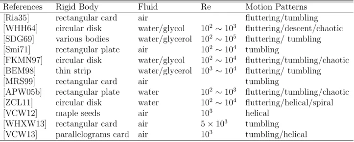
As shown in Table 2.1, scientist did numerous physical experiments of falling rigid body in ﬂuid, and found out the hidden rules as motion patterns inside the daily-life phenomena.

As explained previously, the unsteady dynamics in high Reynolds number flow make the motions seem to be unpredictable. [WHH64] firstly provided a phase diagram based on the Reynolds number Re and the dimensionless moment of inertia I^∗. The stable and unstable oscillations of the body are determined by these two parameters. The tumbling motion happens at both largerReandI^∗. [SDG69] found the effects of the shape of various bodies andReto the dynamics, and declaimed that the motion patterns of a disk are more unstable than the patterns of a three-dimensional sphere. [Smi71] measured the phase diagram for rectangular plates which is similar to the work [WHH64]. [FKMN97] started the further experiments on falling disks, and the apparent chaotic motion is proven to exist. Then, [BEM98] also observed the fluttering and tumbling motions, they discovered the fluttering dynamic of a falling object and the transition from fluttering to tumbling motions occurs at a special dimensionless quantity: the Froude number. [MRS99] studied the dependence of the angular velocity on the width of a tumbling card.

Recent experimental works attempts to uncover the motion patterns in three dimensions and the motion transitions among motion patterns. The experiments in [ZCL11, ZLS⁺13]

have found an additional three typical trajectories in a three-dimensional environment:

zigzag, transitional helix, and spiral motions. The exhaust experimental work [Raz10] concerned about the transitions among diﬀerent motion pattens of leaves based on more than six thousands three-dimensional experiments. In the recent work [VCW12] and [VCW13], the similar patterns of helical motions are observed for diﬀerent shapes of rigid bodies. All the patterns and the experimental environments of previous work are listed in Table 2.1.

Table 2.1: Summary of previous investigations on immersed rigid body dynamics from physical experiments in the order of published years.

References Rigid Body Fluid Re Motion Patterns

[Ria35] rectangular card air ﬂuttering/tumbling

[WHH64] circular disk water/glycol 10² ∼10³ ﬂuttering/descent/chaotic [SDG69] various bodies water/glycerol 10² ∼10⁵ ﬂuttering/ tumbling [Smi71] rectangular plate air 10² ∼10⁴ tumbling

[FKMN97] circular disk water/glycol 10² ∼10⁴ ﬂuttering/tumbling/chaotic [BEM98] thin strip water/glycerol 10³ ∼10⁴ ﬂuttering/ tumbling

[MRS99] rectangular card air tumbling

[APW05b] rectangular plate water 10² ∼10³ ﬂuttering/tumbling/chaotic [ZCL11] circular disk water 10² ∼10⁴ ﬂuttering/helical/spiral

[VCW12] maple seeds air 10³ helical

[WHXW13] rectangular card air 5×10³ tumbling

[VCW13] parallelograms card air 10³ tumbling/helical

(30)

2.2 Related work in physical simulations

In this section, the related works of physical simulations are presented from the research field of both computer graphics and fluid mechanics related to immersed rigid body dynamics. This thesis proposes a family of data-driven methods considering the real flow effects which the previous computer graphics work. The numerical methods in fluid mechanics are mainly in 2D case as shown in Table 2.2. Recent 3D physical simulations have the limitations to account for turbulent flow and the high computational cost, which are not feasible to satisfy the realistic and real-time requirements in this study.

2.2.1 Computer Graphics

Rigid body dynamics has a long history in computer graphics and is a significant start- ing points of other character and deformable body simulations [Bar93]. A recent work [BETC12] detailed the modern development of mechanics, complementarity problems, numerical methods in interactive rigid body simulations. The traditional rigid body solvers do not consider the influences from the surrounding flow, where any rigid body always falls down vertically.

Two-way Coupling simulations between rigid body and incompressible fluid has been studied extensively in computer graphics. Basically there are two types of schemes on this research. The first scheme handles fluid in Euler formulation and rigid bodies in Lagrangian formation [CMT04, GSLF05, BBB07, RMSG⁺08, CM10]. Guendelman et al. [GSLF05] proposed a robust ray casting algorithm for the coupling between fluid and cloths to avoid fluid leaking. Carlson et al. [CMT04] treated the rigid body as fluid grid by using distributed Langrange multiplier. The second scheme is the fully Langrangian meshless method [BTT09, CBP05, SSP07, HLW⁺12]. Becker et al. [BTT09] proposed a direct forcing method in a predictor-corrector scheme with SPH particles. Solenthaler et al. [SSP07] used a penalty method to analyze the forces on the immersed boundary. These two-way coupling approaches provide great simulation results for weakly coupling problems in low-Re conditions, where the rigid body does not exhibit chaotic behaviours. For the research purposes of immersed rigid-body dynamics in this thesis, it is trivial and infeasible to simulate high-Retwo-way coupling with turbulent flow in computer graphics as explained in Chapter 1. It is too computationally heavy for immersed rigid body simulations where the motions of fluids are not visible.

Aerodynamics simulations are widely proposed in computer animation. [WZF⁺04]

proposed Lattice-Boltzmann method for solving ﬂuid simulation and Kutta-Joukowski theorem for body’s dynamics, such as soap bubbles and feathers. This proposed

(31)

method cannot produce a designated motion trajectory, and it has diﬃculty in simulating multiple objects, because this method requires a large computational cost (a single bubble: CPU 2.8 fps and GPU 11.5 fps; a single feather: CPU 0.76 fps and GPU 6.1 fps). The commercial CG tools, including LightWave^{T M} and Maya^@ nCloth^{T M}, do not embody the functions of the animation for immersed rigid body, instead, they provide particle systems to model an immersed body by adjusting the drag and lift parameters in a wind ﬁeld. In all of these works, the motion paths are unpredictable, and it is infeasible to achieve realistic motion.

Unsteady dynamics The underwater simulation work [WP12] introduced a Kirchhoff tensor to represent inertial effects for underwater rigid body simulations. This approach is suitable for the inviscid and irrotational flow with low-Re number.

[OKRC10] presented a fractional derivatives method for representing historic force of underwater cloth in low Reynolds number flow. This work proposes a Langevin model related to the turbulent flow for solving the vortical loads. Langevin model has been applied to enhance turbulent flow simulations [CZY11] and simulations of float- ing lightweight rigid body [YCZ11] in previous work. In these work, the rotational velocity and the coupling between translational and rotational velocities are not concerned. We resolve these issues by combing generalized Kirchhoff equations with Langevin model in this paper. There are also some interesting works about motions of snowflakes and dusts, such as particle system [CFW99, TLP06], spectral-particle method [LZK⁺04]. All these approaches do not take into account the unsteady dynamics of the body, both inertial and viscous effects from the surrounding flow and the influences from the generated turbulences at the body’s boundary layer.

Turbulent Flow simulations are different with direct numerical simulation of Navier- Stokes equations. First, from the view of fluid mechanics, there are some sophisti- cate approaches in this fields, including turbulent-viscosity models (k-ε equations), Reynolds-stress models, Probability Density Function methods (Langevin model) and large-eddy simulation. It is not apparent to adopt these approaches directly in computer animation, and there are some successful works [PTC⁺10, PTSG09] in computer graphics community recently. Note that Langevin model is an empirical model based onk-ε equations [Pop83, Pop11] but an effective Langragian-stochastic approach to represent the dynamics of passive particles in turbulent flow [MD04]. Re- cent work shows that non-spherical particles moving in turbulent flow [MR10] exhibit the similar dynamics of immersed rigid bodies which has been discussed in previous work [XM13]. Therefore, it is physically reasonable to adopt Langevin model for simulating immersed rigid bodies in this work.

Data-driven methods have been proposed based on the Markov model [RP01], captured

(32)

videos [AHN04], segments from ﬂuid simulations [SYWC05], trajectories animated by Maya [VB08], and sketches by a designer [HQHQ10] to simulate the motions of falling leaves. All these simulations ignore the nature of motion of immersed rigid bodies and consider it a completely complex and unpredictable dynamic motion, which is modeled by stochastic processes or a simple particle representation.

Character animation method proposed motion synthesis combining the controllability of procedural and physically-based animation with the realistic appearance of a pre- recorded motion stream (e.g. motion capture). The motion graph [AF02] can au- tomatically organize example motion clips into graphs for eﬃcient motion synthesis.

Later, Kovar et al. built an extended motion graph using local search with a branch and bound algorithm [KGP02]. Besides being used in human motion, motion graphs are also used in other physical simulations, such as tree animation [HFR06, ZZJ⁺07].

This work includes the motion graph technique for synthesizing the motion of immersed rigid body.

2.2.2 Fluid mechanics

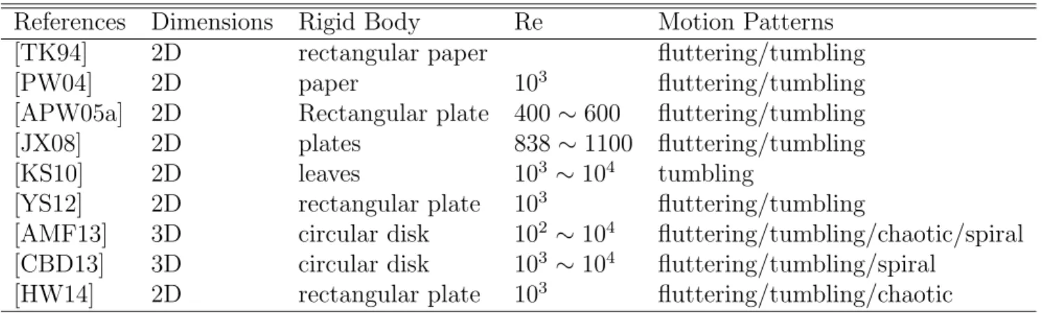
The developments of numerical simulations of immersed rigid body dynamics are listed in Table 2.2. The numerical work [TK94, APW05b, Umb05, PM11, ERFM12] corrected unsteady approximations of drag and lift forces. Tanabe et al. [TK94] built a simple phenomenological model of falling paper by solving ordinary differential equations (ODEs) based on the Kutta-Joukowski theorem. Andersen et al. [PW04] provided a solution of the 2D Navier-Stokes equations for the flow around the tumbling plate, which are solved in the formulation of vorticity stream function within a body-fixed elliptical coordinate system. This method utilized a conformal mapping to avoid singularities. [APW05b] con- ducted various numerical simulation in air, and discussed the motion transition between tumbling and fluttering motion patterns. This work observed the apparently chaotic motions are due to the high sensitivity of the dynamical system to experimental noise. [JX08]

attempted to overcome the various discrepancies between experimental and numerical solutions encountered in [APW05b]. [KS10] developed a Fourier pseudo-spectral method to solve the 2D Navier-Stokes equations coupled with equations which govern free fall motion of a object, and the simulation results varied depending on the Reynolds numbers.

[YS12] presented a direct forcing immersed boundary method for strongly coupling problems, including vortex-induced vibrations of a circular cylinder, transverse and rotational galloping of rectangular bodies, and ﬂuttering and tumbling of rectangular plates. Another approach for solving strongly coupling motions is a point vortex method [MLS09]. This method is based on Brown-Michael equation via Kutta conditions for 2D coupled motion of a sharp-edged rigid body and the surrounding inviscid ﬂow.

(33)

Table 2.2: Summary of previous investigations on immersed rigid body dynamics from numerical experiments in the order of published years.

References Dimensions Rigid Body Re Motion Patterns

[TK94] 2D rectangular paper ﬂuttering/tumbling

[PW04] 2D paper 10³ ﬂuttering/tumbling

[APW05a] 2D Rectangular plate 400∼600 ﬂuttering/tumbling

[JX08] 2D plates 838∼1100 ﬂuttering/tumbling

[KS10] 2D leaves 10³ ∼10⁴ tumbling

[YS12] 2D rectangular plate 10³ ﬂuttering/tumbling

[AMF13] 3D circular disk 10² ∼10⁴ ﬂuttering/tumbling/chaotic/spiral [CBD13] 3D circular disk 10³ ∼10⁴ ﬂuttering/tumbling/spiral

[HW14] 2D rectangular plate 10³ fluttering/tumbling/chaotic Recent progress studied the effects of mass distribution [HLW⁺13], motion transition of motion patterns [HW14]. These works are mainly discover the cases of quasi-two- dimensional setups. The recent work about three-dimensional dynamical motion patterns of immersed rigid body dynamics based on solid-fluid interaction simulations [AMF13, CBD13]. This thesis combines the research results of both experimental and numerical works to seek the motion patterns and their motion transition for an individual body in three dimensions. [CBD13] investigated the motion transitions among motion patterns based on the Galileo number and the non-dimensionalized mass. The numerical simulations of solid-fluid interaction utilized spectral element method with domain decomposition.

[AMF13] studied the inﬂuence of the body density and the thickness of disk to the motion transitions by simulating the coupled Navier-Stokes equations with generalized Kirchhoﬀ equations of rigid body dynamics [MM02].

2.3 Basic physics of immersed rigid body dynamics

2.3.1 Rigid body equations

Without the consideration of fluid effects, the dynamics of 3D rigid body follows the Newton-Euler equations in body-fixed frame.

F = ma_cm−mg (2.1)

τ = Iω˙ +ω×Iω (2.2)

whereF and τ are the aerodynamics forces and torques, respectively. m and I is the mass and moment of inertia of the rigid body. ωdenotes angular velocity. a_cmis the translational

(34)

acceleration at center of mass in body-ﬁxed frame and the value becomesacm= ˙v+ω×v by coordinate transformation from the world-frame, v is the translational velocity of the body. Finally, the rigid body equations can be described as:

( F

τ )

= (

mE 0

0 I

) (

˙ v

˙ ω

) +

(

ω×mEv ω×Iω

)

(2.3) whereE is identity matrix.

2.3.2 Coupling equations of ﬂuid-body system

The Navier-Stoke Equations are transformed into the following formulations in the reference frame moving with the rigid body.

∂u

∂t +ω×u+∇ ·(u(u−w)) = 1

ρ_f∇p+ν∇²u (2.4)

∇ ·u = 0 (2.5)

where u and p are the velocity field in the flow. ρ_f and ν are the density and viscosity of the flow. w=v+ω×r is the body velocity in world-frame, and r denotes the orthogonal coordinate in body-fixed frame. On the body boundary S, the flow velocity satisfies the no-slip boundary condition.

u(x) = w(x) ∀x∈S (2.6)

Then, the aerodynamic force and torque on the body are given as follows:

F =

∫

S

(σ·n)ds (2.7)

τ =

∫

S

x×(σ·n)ds (2.8)

whereσ =−pE+ρfν(∇v+∇^Tv) is the stress tensor of the ﬂow,n is the local normal to the solid boundary.

2.3.3 Motions in potential ﬂow

In the case of the aforementioned coupling equation (Equation 2.5) in zero viscosity, the coupling problem can be converted a ﬂow potential ϕ that satisﬁes the following Laplace

(35)

problem if the ﬂow is irrotational from rest.

∇²ϕ(x) = 0 ∀x∈R³B (2.9)

∂ϕ(x)

∂n = w(x)·n ∀x∈S (2.10)

ϕ(x) = 0 ∀∥x∥ → ∞ (2.11)

Here B represents the domain of rigid body. Note that the non-slip boundary conditions in Equation 2.6 should be replaced by Neumann conditions in the inviscid limit.

In terms of the inviscid theory [Lam75], the dynamics of rigid body inside potential ﬂow is given as Kirchhoﬀ Equations:

( F

τ )

= (

mE+K11 K12 K21 I+K22

) (

˙ v

˙ ω

) +

(

ω×(mE+K11)v ω×(I+K22)ω+v×(K11v)

)

(2.12) where K is a symmetric added-mass tensor, i.e.,K21 =K12^T.

K = (

K11 K12 K21 K22

)

K_ij =ρ_f

∫

S

ϕ_i∂ϕ_j

∂nds (2.13)

More details about the added-mass tensor can be found in [New77].

2.3.4 Experimental force model in 2D real ﬂow

The real ﬂow is viscous and vorticity exists around the immersed rigid body. The existence of vorticity in the ﬂow makes the immersed rigid body dynamics complicated to analyse.

For 2D situations, an approximation of the aerodynamic forces and torques is proposed by [APW05b, APW05a, Umb05]. The 2D dynamical model is given as follows:

(m+m11) ˙v_x = F_x−F_Lsinα−F_Dcosα−m_bgsinθ (2.14) (m+m22) ˙vy = Fy+FLcosα−FDsinα−mbgcosθ (2.15)

(I+I_a) ˙ω = M_a−M_s (2.16)

θ˙ = ω (2.17)

wherem_b is the buoyancy-corrected gravitational force. m11, m22 and I_a are the diagonal components in added-mass tensor. F_x = (m+m22)ωv_y, F_y =−(m+m11)ωv_x and M_a = (m11−m22)v_xv_y are the forces and torque due to added mass. θ andα are the angle and