Optimizing Segmentation Strategies for Simultaneous Speech Translation
Yusuke Oda Graham Neubig Sakriani Sakti Tomoki Toda Satoshi Nakamura Graduate School of Information Science
Nara Institute of Science and Technology Takayama, Ikoma, Nara 630-0192, Japan
{oda.yusuke.on9, neubig, ssakti, tomoki, s-nakamura}@is.naist.jp
Abstract
In this paper, we propose new algorithms for learning segmentation strategies for si- multaneous speech translation. In contrast to previously proposed heuristic methods, our method finds a segmentation that di- rectly maximizes the performance of the machine translation system. We describe two methods based on greedy search and dynamic programming that search for the optimal segmentation strategy. An experi- mental evaluation finds that our algorithm is able to segment the input two to three times more frequently than conventional methods in terms of number of words, while maintaining the same score of auto- matic evaluation.
11 Introduction
The performance of speech translation systems has greatly improved in the past several years, and these systems are starting to find wide use in a number of applications. Simultaneous speech translation, which translates speech from the source language into the target language in real time, is one example of such an application. When translating dialogue, the length of each utterance will usually be short, so the system can simply start the translation process when it detects the end of an utterance. However, in the case of lectures, for example, there is often no obvious boundary between utterances. Thus, translation systems re- quire a method of deciding the timing at which to start the translation process. Using estimated ends of sentences as the timing with which to start translation, in the same way as a normal text trans- lation, is a straightforward solution to this problem (Matusov et al., 2006). However, this approach
1The implementation is available at
http://odaemon.com/docs/codes/greedyseg.html.
impairs the simultaneity of translation because the system needs to wait too long until the appearance of a estimated sentence boundary. For this reason, segmentation strategies, which separate the input at appropriate positions other than end of the sen- tence, have been studied.
A number of segmentation strategies for simul- taneous speech translation have been proposed in recent years. F¨ugen et al. (2007) and Bangalore et al. (2012) propose using prosodic pauses in speech recognition to denote segmentation boundaries, but this method strongly depends on characteris- tics of the speech, such as the speed of speaking.
There is also research on methods that depend on linguistic or non-linguistic heuristics over recog- nized text (Rangarajan Sridhar et al., 2013), and it was found that a method that predicts the location of commas or periods achieves the highest perfor- mance. Methods have also been proposed using the phrase table (Yarmohammadi et al., 2013) or the right probability (RP) of phrases (Fujita et al., 2013), which indicates whether a phrase reorder- ing occurs or not.
However, each of the previously mentioned methods decides the segmentation on the basis of heuristics, so the impact of each segmenta- tion strategy on translation performance is not di- rectly considered. In addition, the mean number of words in the translation unit, which strongly af- fects the delay of translation, cannot be directly controlled by these methods.
2In this paper, we propose new segmentation al- gorithms that directly optimize translation perfor- mance given the mean number of words in the translation unit. Our approaches find appropri- ate segmentation boundaries incrementally using greedy search and dynamic programming. Each boundary is selected to explicitly maximize trans-
2The method using RP can decide relative frequency of segmentation by changing a parameter, but guessing the length of a translation unit from this parameter is not trivial.
551
lation accuracy as measured by BLEU or another evaluation measure.
We evaluate our methods on a speech transla- tion task, and we confirm that our approaches can achieve translation units two to three times as fine- grained as other methods, while maintaining the same accuracy.
2 Optimization Framework
Our methods use the outputs of an existing ma- chine translation system to learn a segmentation strategy. We define
F = {fj : 1 ≤ j ≤ N}, E = {ej : 1 ≤ j ≤ N}as a parallel corpus of source and target language sentences used to train the segmentation strategy.
Nrepresents the number of sentences in the corpus. In this work, we consider sub-sentential segmentation, where the input is already separated into sentences, and we want to further segment these sentences into shorter units. In an actual speech translation sys- tem, these sentence boundaries can be estimated automatically using a method like the period es- timation mentioned in Rangarajan Sridhar et al.
(2013). We also assume the machine translation system is defined by a function
MT(f)that takes a string of source words
fas an argument and re- turns the translation result
e.ˆ3We will introduce individual methods in the fol- lowing sections, but all follow the general frame- work shown below:
1. Decide the mean number of words
µand the machine translation evaluation measure
EVas parameters of algorithm. We can use an automatic evaluation measure such as BLEU (Papineni et al., 2002) as
EV. Then, we cal- culate the number of sub-sentential segmen- tation boundaries
Kthat we will need to in- sert into
Fto achieve an average segment length
µ:K:= max (
0,
⌊∑
f∈F|f| µ
⌋
−N )
.
(1) 2. Define
Sas a set of positions in
Fin which we will insert segmentation boundaries. For example, if we will segment the first sentence after the third word and the third sentence af- ter the fifth word, then
S = {⟨1,3⟩,⟨3,5⟩}.3In this work, we do not use the history of the language model mentioned in Bangalore et al. (2012). Considering this information improves the MT performance and we plan to include this in our approach in future work.
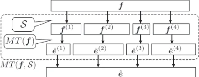
Figure 1: Concatenated translation
MT(f,S).Based on this representation, choose
Kseg- mentation boundaries in
Fto make the set
S∗that maximizes an evaluation function
ωas below:
S∗:= arg max
S∈{S′:|S′|=K}ω(S;F,E, EV, MT).
(2) In this work, we define
ωas the sum of the evaluation measure for each parallel sentence pair
⟨fj,ej⟩:ω(S) :=∑N
j=1
EV(MT(fj,S),ej),
(3) where
MT(f,S)represents the concatena- tion of all partial translations
{MT(f(n))}given the segments
Sas shown in Figure 1.
Equation (3) indicates that we assume all parallel sentences to be independent of each other, and the evaluation measure is calcu- lated for each sentence separately. This lo- cality assumption eases efficient implementa- tion of our algorithm, and can be realized us- ing a sentence-level evaluation measure such as BLEU+1 (Lin and Och, 2004).
3. Make a segmentation model
MS∗by treating the obtained segmentation boundaries
S∗as positive labels, all other positions as negative labels, and training a classifier to distinguish between them. This classifier is used to de- tect segmentation boundaries at test time.
Steps 1. and 3. of the above procedure are triv-
ial. In contrast, choosing a good segmentation ac-
cording to Equation (2) is difficult and the focus
of the rest of this paper. In order to exactly solve
Equation (2), we must perform brute-force search
over all possible segmentations unless we make
some assumptions about the relation between the
ωyielded by different segmentations. However,
the number of possible segmentations is exponen-
tially large, so brute-force search is obviously in-
tractable. In the following sections, we propose 2
I ate lunch but she left Segments already selected at the k-th iteration
ω = 0.5 ω = 0.8 (k+1)-th segment
ω = 0.7
Figure 2: Example of greedy search.
Algorithm 1 Greedy segmentation search
S∗ ←∅for
k= 1to
Kdo
S∗← S∗∪{
arg max
s∈S∗
ω(S∗∪ {s}) }
end for return
S∗methods that approximately search for a solution to Equation (2).
2.1 Greedy Search
Our first approximation is a greedy algorithm that selects segmentation boundaries one-by-one. In this method,
kalready-selected boundaries are left unchanged when deciding the
(k+1)-th boundary.We find the unselected boundary that maximizes
ωand add it to
S:
Sk+1=Sk∪ {
arg max
s∈Sk
ω(Sk∪ {s}) }
.
(4) Figure 2 shows an example of this process for a single sentence, and Algorithm 1 shows the algo- rithm for calculating
Kboundaries.
2.2 Greedy Search with Feature Grouping and Dynamic Programming
The method described in the previous section finds segments that achieve high translation per- formance for the training data. However, because the translation system
MTand evaluation mea- sure
EVare both complex, the evaluation function
ωincludes a certain amount of noise. As a result, the greedy algorithm that uses only
ωmay find a segmentation that achieves high translation perfor- mance in the training data by chance. However, these segmentations will not generalize, reducing the performance for other data.
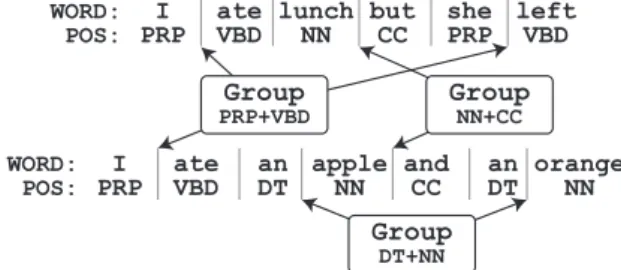
We can assume that this problem can be solved by selecting more consistent segmentations of the training data. To achieve this, we introduce a con- straint that all positions that have similar charac- teristics must be selected at the same time. Specif- ically, we first group all positions in the source
I ate lunch but she left PRP VBD NN CC PRP VBD
I ate an apple and an orange PRP VBD DT NN CC DT NN WORD:
POS:
WORD:
POS:
Group PRP+VBD
Group NN+CC
Group DT+NN
Figure 3: Grouping segments by POS bigrams.
sentences using features of the position, and intro- duce a constraint that all positions with identical features must be selected at the same time. Figure 3 shows an example of how this grouping works when we use the POS bigram surrounding each potential boundary as our feature set.
By introducing this constraint, we can expect that features which have good performance over- all will be selected, while features that have rela- tively bad performance will not be selected even if good performance is obtained when segmenting at a specific location. In addition, because all posi- tions can be classified as either segmented or not by evaluating whether the corresponding feature is in the learned feature set or not, it is not necessary to train an additional classifier for the segmenta- tion model when using this algorithm. In other words, this constraint conducts a kind of feature selection for greedy search.
In contrast to Algorithm 1, which only selected one segmentation boundary at once, in our new setting there are multiple positions selected at one time. Thus, we need to update our search algo- rithm to handle this setting. To do so, we use dynamic programming (DP) together with greedy search. Algorithm 2 shows our Greedy+DP search algorithm. Here,
c(ϕ;F)represents the number of appearances of
ϕin the set of source sentences
F, andS(F,Φ)represents the set of segments de- fined by both
Fand the set of features
Φ.The outer loop of the algorithm, like Greedy, iterates over all
Sof size 1 to
K. The inner loopexamines all features that appear exactly
jtimes in
F, and measures the effect of adding them to the best segmentation with
(k−j)boundaries.
2.3 Regularization by Feature Count
Even after we apply grouping by features, it
is likely that noise will still remain in the less
frequently-seen features. To avoid this problem,
we introduce regularization into the Greedy+DP
algorithm, with the evaluation function
ωrewrit-
Algorithm 2 Greedy+DP segmentation search
Φ0 ←∅for
k= 1to
Kdo for
j = 0to
k−1do
Φ′ ← {ϕ:c(ϕ;F) =k−j∧ϕ∈Φj} Φk,j←Φj∪
{ arg max
ϕ∈Φ′ ω(S(F,Φj∪ {ϕ})) }
end for
Φk← arg max
Φ∈{Φk,j:0≤j<k}ω(S(F,Φ))
end for
return
S(F,ΦK)ten as below:
ωα(Φ) :=ω(S(F,Φ))−α|Φ|.
(5) The coefficient
αis the strength of the regulariza- tion with regards to the number of selected fea- tures. A larger
αwill result in a larger penalty against adding new features into the model. As a result, the Greedy+DP algorithm will value fre- quently appearing features. Note that the method described in the previous section is equal to the case of
α= 0in this section.
2.4 Implementation Details
Our Greedy and Greedy+DP search algorithms are completely described in Algorithms 1 and 2.
However, these algorithms require a large amount of computation and simple implementations of them are too slow to finish in realistic time. Be- cause the heaviest parts of the algorithm are the calculation of
MTand
EV, we can greatly im- prove efficiency by memoizing the results of these functions, only recalculating on new input.
3 Experiments
3.1 Experimental Settings
We evaluated the performance of our segmentation strategies by applying them to English-German and English-Japanese TED speech translation data from WIT3 (Cettolo et al., 2012). For English- German, we used the TED data and splits from the IWSLT2013 evaluation campaign (Cettolo et al., 2013), as well as 1M sentences selected from the out-of-domain training data using the method of Duh et al. (2013). For English-Japanese, we used TED data and the dictionary entries and sen- tences from EIJIRO.
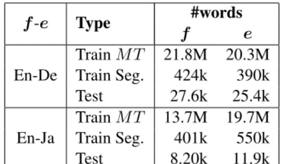
4Table 1 shows summaries of the datasets we used.
4http://eowp.alc.co.jp/info2/
f
-e Type #words
f e
En-De Train
MT21.8M 20.3M Train Seg. 424k 390k
Test 27.6k 25.4k
En-Ja Train
MT13.7M 19.7M Train Seg. 401k 550k
Test 8.20k 11.9k
Table 1: Size of
MTtraining, segmentation train- ing and testing datasets.
We use the Stanford POS Tagger (Toutanova et al., 2003) to tokenize and POS tag English and German sentences, and KyTea (Neubig et al., 2011) to tokenize Japanese sentences. A phrase- based machine translation (PBMT) system learned by Moses (Koehn et al., 2007) is used as the trans- lation system
MT. We use BLEU+1 as the eval- uation measure
EVin the proposed method. The results on the test data are evaluated by BLEU and RIBES (Isozaki et al., 2010), which is an evalu- ation measure more sensitive to global reordering than BLEU.
We evaluated our algorithm and two conven- tional methods listed below:
Greedy is our first method that uses simple greedy search and a linear SVM (using surrounding word/POS 1, 2 and 3-grams as features) to learn the segmentation model.
Greedy+DP is the algorithm that introduces grouping the positions in the source sentence by POS bigrams.
Punct-Predict is the method using predicted po- sitions of punctuation (Rangarajan Sridhar et al., 2013).
RP is the method using right probability (Fujita et al., 2013).
3.2 Results and Discussion
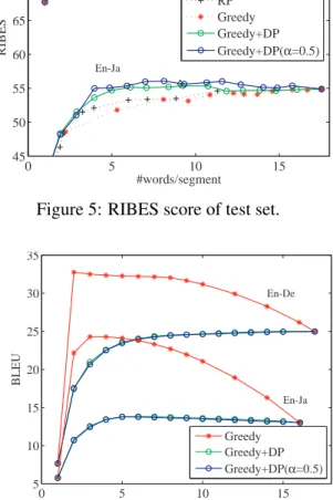
Figures 4 and 5 show the results of evaluation for each segmentation strategy measured by BLEU and RIBES respectively. The horizontal axis is the mean number of words in the generated transla- tion units. This value is proportional to the delay experienced during simultaneous speech transla- tion (Rangarajan Sridhar et al., 2013) and thus a smaller value is desirable.
RP, Greedy, and Greedy+DP methods have
multiple results in these graphs because these
methods have a parameter that controls segmen-
tation frequency. We move this parameter from
no segmentation (sentence-based translation) to
0 5 10 15 10
12 14 16 18 20
En-De
En-Ja
#words/segment
BLEU
Punct-Predict RP Greedy Greedy+DP Greedy+DP(α=0.5)
Figure 4: BLEU score of test set.
0 5 10 15
45 50 55 60 65 70 75 80
En-De
En-Ja
#words/segment
RIBES
Punct-Predict RP Greedy Greedy+DP Greedy+DP(α=0.5)
Figure 5: RIBES score of test set.
segmenting every possible boundary (word-based translation) and evaluate the results.
First, focusing on the Greedy method, we can see that it underperforms the other methods. This is a result of over-fitting as will be described in detail later. In contrast, the proposed Greedy+DP method shows high performance compared to the other methods. Especially, the result of BLEU on the English-German and the RIBES on both lan- guage pairs show higher performance than RP at all speed settings. Punct-Predict does not have an adjustable parameter, so we can only show one point. We can see that Greedy+DP can be- gin translation about two to three times faster than Punct-Predict while maintaining the same perfor- mance.
Figure 6 shows the BLEU on the training data.
From this figure, it is clear that Greedy achieves much higher performance than Greedy+DP. From this result, we can see that the Greedy algorithm is choosing a segmentation that achieves high accu- racy on the training data but does not generalize to the test data. In contrast, the grouping constraint in the Greedy+DP algorithm is effectively suppress- ing this overfitting.
The mean number of words
µcan be decided independently from other information, but a con- figuration of
µaffects tradeoff relation between translation accuracy and simultaneity. For exam- ple, smaller
µmakes faster translation speed but it also makes less translation accuracy. Basically, we should choose
µby considering this tradeoff.
4 Conclusion and Future Work
We proposed new algorithms for learning a seg- mentation strategy in simultaneous speech trans-
0 5 10 15
5 10 15 20 25 30 35
En-De
En-Ja
#words/segment
BLEU
Greedy Greedy+DP Greedy+DP(α=0.5)
Figure 6: BLEU score of training set.
lation. Our algorithms directly optimize the per- formance of a machine translation system accord- ing to an evaluation measure, and are calculated by greedy search and dynamic programming. Exper- iments show our Greedy+DP method effectively separates the source sentence into smaller units while maintaining translation performance.
With regards to future work, it has been noted that translation performance can be im- proved by considering the previously translated segment when calculating LM probabilities (Ran- garajan Sridhar et al., 2013). We would like to ex- pand our method to this framework, although in- corporation of context-sensitive translations is not trivial. In addition, the Greedy+DP algorithm uses only one feature per a position in this paper. Using a variety of features is also possible, so we plan to examine expansions of our algorithm to multiple overlapping features in future work.
Acknowledgements
Part of this work was supported by JSPS KAK-
ENHI Grant Number 24240032.
References
Srinivas Bangalore, Vivek Kumar Rangarajan Srid- har, Prakash Kolan, Ladan Golipour, and Aura Jimenez. 2012. Real-time incremental speech-to- speech translation of dialogs. InProc. NAACL HLT, pages 437–445.
Mauro Cettolo, Christian Girardi, and Marcello Fed- erico. 2012. Wit3: Web inventory of transcribed and translated talks. InProc. EAMT, pages 261–268.
Mauro Cettolo, Jan Niehues, Sebastian St¨uker, Luisa Bentivogli, and Marcello Federico. 2013. Report on the 10th iwslt evaluation campaign. InProc. IWSLT.
Kevin Duh, Graham Neubig, Katsuhito Sudoh, and Ha- jime Tsukada. 2013. Adaptation data selection us- ing neural language models: Experiments in ma- chine translation. InProc. ACL, pages 678–683.
Christian F¨ugen, Alex Waibel, and Muntsin Kolss.
2007. Simultaneous translation of lectures and speeches. Machine Translation, 21(4):209–252.
Tomoki Fujita, Graham Neubig, Sakriani Sakti, Tomoki Toda, and Satoshi Nakamura. 2013. Sim- ple, lexicalized choice of translation timing for si- multaneous speech translation. InInterSpeech.
Hideki Isozaki, Tsutomu Hirao, Kevin Duh, Katsuhito Sudoh, and Hajime Tsukada. 2010. Automatic evaluation of translation quality for distant language pairs. InProc. EMNLP, pages 944–952.
Philipp Koehn, Hieu Hoang, Alexandra Birch, Chris Callison-Burch, Marcello Federico, Nicola Bertoldi, Brooke Cowan, Wade Shen, Christine Moran, Richard Zens, Chris Dyer, Ondˇrej Bojar, Alexandra Constantin, and Evan Herbst. 2007. Moses: Open source toolkit for statistical machine translation. In Proc. ACL, pages 177–180.
Chin-Yew Lin and Franz Josef Och. 2004. Orange: A method for evaluating automatic evaluation metrics for machine translation. InProc. COLING.
Evgeny Matusov, Arne Mauser, and Hermann Ney.
2006. Automatic sentence segmentation and punc- tuation prediction for spoken language translation.
InProc. IWSLT, pages 158–165.
Graham Neubig, Yosuke Nakata, and Shinsuke Mori.
2011. Pointwise prediction for robust, adaptable japanese morphological analysis. In Proc. NAACL HLT, pages 529–533.
Kishore Papineni, Salim Roukos, Todd Ward, and Wei- Jing Zhu. 2002. Bleu: A method for automatic eval- uation of machine translation. InProc. ACL, pages 311–318.
Vivek Kumar Rangarajan Sridhar, John Chen, Srinivas Bangalore, Andrej Ljolje, and Rathinavelu Chengal- varayan. 2013. Segmentation strategies for stream- ing speech translation. InProc. NAACL HLT, pages 230–238.
Kristina Toutanova, Dan Klein, Christopher D. Man- ning, and Yoram Singer. 2003. Feature-rich part-of- speech tagging with a cyclic dependency network.
InProc. NAACL, pages 173–180.
Mahsa Yarmohammadi, Vivek Kumar Rangara- jan Sridhar, Srinivas Bangalore, and Baskaran Sankaran. 2013. Incremental segmentation and decoding strategies for simultaneous translation. In Proc. IJCNLP, pages 1032–1036.