Instructions for use
A uthor(s ) K A NG,HUNS E OK
C itation Hokkaido University Preprint S eries in Mathematics, 931: 1-20
Is s ue D ate 2008-12-8
D O I 10.14943/84079
D oc UR L http://hdl.handle.net/2115/69739
T ype bulletin (article)
F ile Information pre931.pdf
HUNSEOK KANG
Abstract. In this paper, a discrete version of a reaction-diffusion equation, also known as coupled map lattice (CML), which corresponds to the Tur-ing model of morphogenesis is studied. It is shown that CML possesses a hyperbolic property displaying a type of spatio-temporal chaos. Through-out a mathematical background of hyperbolic properties in lattice dynamical systems which are related to spatio-temporal chaos, a mathematical proof is given that the CML obtained from the Turing model possesses such hyperbolic properties. Finally, numerical studies of this finding in varying parameters to present a variety of chaotic behaviors of this system is performed.
1. Introduction
In 1952, A. Turing proposed a theoretical model for spatial pattern formation using reaction-diffusion mechanism. In his work [16] and its extensions [5, 10], it was shown that the diffusion in the mechanism may break stability in the system of reacting chemicals, and that this diffusion-driven instability results in spatially periodic patterns that are stationary in time. One of the remarkable features in this system is that the resulting pattern formation arises autonomously without referring to any external sources, such as length scales or constraints.
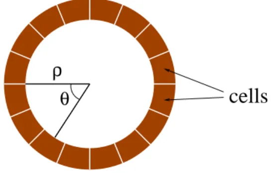
The morphogenesis is an embryological development of the structure of an organ-ism or some part of an organorgan-ism. Turing suggested a model of an idealized embryo which contains two characteristic chemical substancesX andYcalledmorphogens. These substances react with each other in each cell and diffuse between neighbor-ing cells with diffusibility coefficients µand ν respectively. Consider an idealized embryo which is realized as an annulus of the inner radiusρof tissue (see Figure 1). Concentrations of the corresponding chemicalsX andY are denoted byX and
Y, respectively. LetK1(X, Y) andK2(X, Y) be kinetic functions representing the rates at which concentrationsX and Y, respectively, change due to the chemical interaction.
The reaction rates are assumed to obey thelaw of mass actionthat states the rate at which a reaction takes place is proportional to the concentrations of the reacting substances. It is also assumed that diffusion obeys the ordinary law of diffusion. In this case, each morphogen moves from the region of greater concentration to the region of lesser one at a rate proportional to the gradient of the concentration.
1991Mathematics Subject Classification. 37N25, 37N10, 35K57.
Key words and phrases. Turing Model, Coupled Map Lattices, Traveling Wave, Hyperbolic set, Smale-horseshoe, Spatio-Temporal Chaos.
cells
θ
ρ
Figure 1. Turing’s model of an idealized embryo.
Then the governing equations are
Xt=K1(X, Y) +
µ ρ2Xθθ,
Yt=K2(X, Y) +
ν ρ2Yθθ,
(1.1)
whereθ is the angle between the radius to the current point and a fixed reference radius. Nonlinearity of the kinetic functions in (1.1) is an essential ingredient and is a source of the instability in the system. Turing used the following formulas for the kinetic functions
K1(X, Y) =−AX2−BXY +C,
K2(X, Y) =AX2+BXY −DY +E,
(1.2)
whereA, B,C,D,E∈R+ are parameters of the reaction in (1.1).
We shall discuss the dynamics of a discrete version of the Turing continuous model of the idealized embryo. When a reaction-diffusion equation is discretized, it forms a CML as usual. When discretizing Equation (1.1) the following discretiza-tions are employed: For the time derivative in (1.1)
(1.3) ∂u(x, t)
∂t →
u(x, t+ ∆t)−u(x, t)
∆t .
And for the space derivative
(1.4) ∂
2u(x, t)
∂x2 →
u(x+ ∆x, t)−2u(x, t) +u(x−∆x, t)
(∆x)2 .
By plugging the discretizations (1.3) and (1.4) into the system (1.1), we obtain a coupled map lattice (CML) of the type:
(1.5) uj(n+ 1) =f(uj(n)) +ǫgj({ui(n)}|i−j|≤s),
wheren∈Zis the discrete time coordinate andj∈Zthe discrete space coordinate. Furthermore,f :R2→R2is thelocal map for the CML and is given by
(1.6) f(u1, u2) = (u1−au21−bu1u2+c, au21+bu1u2+ (1−d)u2+e),
wherea=A∆t >0,b=B∆t >0,c=C∆t >0,d=D∆t >0 ande=E∆t >0 are parameters. Finally,g : (R2)2s+1 →R2 is the interaction of finite size s. By
Referred to Turing’s works, a number of reaction-diffusion models have been proposed for pattern formations. These all rely on the diffusion-driven instability mechanism proposed by Turing, differing only in the terms that govern reaction kineticsK1andK2of (1.1), like in (1.2). A considerable amount of existing works on the proposed models have been mostly involved in numerical and experimental approaches to study spatio-temporal dynamics ([9], [11], [15], etc.). Throughout the study, using dynamical system approaches on the basis of mathematical definitions and proofs, we shall analyze spatio-temporal chaotic dynamics which is physically observable in a finite-dimensional phase space.
The main goal of this paper is to study the dynamics of the local mapf (1.6), focusing on its hyperbolic structure, and finally to show that the lattice system (1.5) displays spatio-temporal chaos. In [13], it was shown that a lattice system obtained from the discretization of the Maginu model of morphogenesis displays spatio-temporal chaos. This model is described by a two-dimensional nonlinear reaction diffusion equation in the Turing form of (1.1) with the reaction kinetic functions K1 andK2
K1(X, Y) =−aX(X−θ)(X−1)−bY, K2(X, Y) =cX−dY.
This Maginu model is a simplified version of the Turing model, which is proposed by Maginu on the basis of FighHugh-Nagumo equation. (See [10] for details.) It was proven that the CML corresponding to this model displays spatio-temporal chaos by showing that the local map of the CML possesses a locally maximal hyperbolic set. This example had been the only known example of lattice system whose local map is hyperbolic. Let us emphasize that the CML corresponding to Turing model also exhibits spatio-temporal chaos as so does its simplified model.
2. Review of Spatio-Temporal Chaos in Lattice Systems
In this section, we describe hyperbolic properties of CMLs via traveling waves, which characterize instability of trajectories. Our goal in this section is to illus-trate that for sufficiently small interactions, these properties are dominated by the hyperbolic behavior of the local mapf and lead to a type of spatio-temporal chaos in lattice systems.
We provide a formal mathematical description of lattice systems for one-dimensional case in terms of dynamical systems. (See [14] for general description of lattice sys-tems for multi-dimensional cases.) We define a special norm called norm with weights. Namely, givenq1>1,q2>1 andu= (uj)∈NZRd,j ∈Z,
kukq1,q2=
X
j<0 |uj|
q−1j
+X
j≥0 |uj|
qj2 .
Then the CML (1.5) is described as the infinite-dimensional dynamical system (Mq1,q2,Φǫ) with the underlying phase space
Mq1,q2 ={u= (uj) :kukq1,q2 <∞}
and the nonlinear evolution operator Φ = Φǫ
It is noted that the dynamical system (Mq1,q2,Φ) corresponds to solutions of the
CML which satisfy the initial condition (uj(0))∈ Mq1,q2 and boundary condition kukq1,q2 <∞.
In [1], traveling wave solution was introduced as a class of solutions for the equation (1.5). Let m and l be relatively prime integers. Then a traveling wave solution of Equation (1.5) is a solution of the form:
uj(n) =ψ(lj+mn),
where ψ: Z→Rd is a function. The numbers mand l determine the velocity of the wave. We assumem > ls, therefore, the velocity of the wave is large.
We consider the traveling wave mapFǫ: (Rd)ls+m→(Rd)ls+m given by
Fǫ(x1, ..., xls+m) = (x2, ..., xls+m, f(xls+1) +ǫg(xp(i))si=−s),
wherep(i) =l(s+i) + 1. Then it was shown that the traveling wave mapFǫ and the evolution operator Φ are conjugated.
Theorem 2.1 (see [1]). There existq1(0)>1,q (0)
2 >1 such that for anyq1> q (0) 1 , q2> q2(0), the traveling wave mapFǫis smoothly conjugate to the evolution operator Φ; in other words, there exists a smooth embeddingχof(Rd)ls+mintoM
q1,q2 such that the following diagram is commutative:
(Rd)ls+m −−−−→ Aχ
q1,q2 ⊂ Mq1,q2
Fǫ m
y
yΦ
(Rd)ls+m −−−−→ Aχ
q1,q2 ⊂ Mq1,q2
whereAq1,q2 =χ((R
d)ls+m)is finite-dimensional.
Consequently, under the assumption that the interaction in (1.5) is sufficiently small, the dynamics of the evolution operator Φ on the set of traveling wave so-lutions with a given velocity m/l is completely determined by the traveling wave mapFǫ.
The evolution operator Φ has a special form Φ =F+ǫGwhereF =N
i∈Zfiand
G= (gj)j∈Z. F is called the uncoupled map andGthe interaction. Iterates of the map Φ generates aZ-action onMq1,q2 called time translation. On the other hand,
we consider another group action of the latticeZ onMq1,q2 by space translations Sk. Namely, for any k∈
Z andu= (uj)∈ Mq1,q2, we set (S
k(u))
i =ui+k. IfG commutes with the spatial translationsSk, i.e.,Sk◦G=G◦Sk, we callGspatial translation invariant. In this case the pairτ = (Φ, S) generates a Z2-action which represents a CML onM.
In [14], a mathematical definition of spatio-temporal chaos in lattice systems is given by Pesin and Sinai. A lattice dynamical system (Φ, S) is said to display
(1) temporal chaos if there exists a measure µ invariant under the Z-action
{Φl}which is mixing;
(2) spatial chaos if there exists a measureµinvariant under theZ-action{Sk} which is mixing;
We consider the case when the local mapf possesses a locally maximal hyperbolic set Λ. In particular, if the local map is hyperbolic in a strong sense (i.e., it possesses a hyperbolic set; every trajectory in this set is highly unstable; see below) then so are the traveling wave map and the restrictions of space and time translations to the submanifold of traveling wave solutions. This implies that the CML displays chaotic behavior of the highest degree, i.e., there exists a measure invariant under space and time translations which is supported on the set of traveling wave solutions and has ergodic properties of higher order.
Recall that a compact invariant set Λ is calledhyperbolic if for every x∈ Λ there exists a splitting of the tangent space TxM at xinto two subspaces Es(x) andEu(x),T MΛ=Es(x)L
Eu(x) such that:
(1) the splitting is invariant under the differentialdf , i.e.,
df(Es(x)) =Es(f(x)), df(Eu(x)) =Eu(f(x));
(2) the subspacesEs(x) andEu(x) are respectively stable and unstable for the differentialdf, i.e.,
|dfn xv| ≤cλ
n|v|
for everyv∈Es(x) and
|dfn
xv| ≥c−1λ− n|v|
for everyv∈Eu(x), wherec >0 and 0< λ <1 are constants independent ofxandv.
A hyperbolic set Λ is said to be locally maximal if there exists an open neigh-borhoodV of Λ such that
Λ = ∞ \
n=−∞
fn(V).
For every pointx∈Λ one can construct local stable and unstable manifolds. We denote them by Ws
loc(x, f) andW u
loc(x, f) respectively. The local stable manifold consists of those pointsywhose forward trajectories follow the trajectory ofxwithin the distanceǫfor sufficiently smallǫ. The local unstable manifold is characterized in a similar way by reversing the time.
One can view the mapFǫ as a small perturbation of the mapF0:
F0(x1, ...xk, ..., xn) = (x2, ..., xk+1, ..., f(xk)).
Note that the mapF0 is an endomorphism and its differential dxF0 is degenerate for everyx∈(Rd)ls+m. Therefore, in studying topological and ergodic properties of the mapFǫ for sufficiently smallǫthe classical perturbation theory may not be applied directly and may need significant modifications.
Assume that Λ is a locally maximal hyperbolic set for the local mapf. Consider the set ˜Λ0 = Nni=1Λi, where Λi are copies of Λi, i = 1, ..., n. We have that
F0(˜Λ0)⊂Λ˜0 and ˜Λ0 is hyperbolic.
The set ˜Λ0 may not survive under small perturbations of F0 (even for local
diffeomorphisms). Therefore, we introduce the set
Λ0=
\
j≥0
It is invariant under F0, i.e.,F0(Λ0) ⊂Λ0. It is locally maximal and hyperbolic,
and it admits the following characterization: For anyy∈Λ0there exists a sequence yk ∈Λ0 such thaty0=y andF0(yk) =yk+1 fork∈Z.
In the case of endomorphisms for every pointxin a locally maximal hyperbolic set one can construct a local stable manifold. It is uniquely defined and consists of those pointsy whose forward trajectories follow the trajectory of xwithin the distanceǫfor sufficiently smallǫ. On the other hand there are many local unstable manifolds, each corresponds to a branch of preimages of x. We will specify later the choice of unstable manifolds.
For the endomorphismF0, the local stable manifold at a pointx= (xi)∈Λ0 is
given by
Ws
loc(x, F0) = k−1
Y
i=1
B(xi, ǫ)× n
Y
i=k
Ws
loc(xi, f),
whereǫ >0 is sufficiently small. We will define the local unstable manifold atxby
Wlocu (x, F0) = k−1
Y
i=1 {xi} ×
n
Y
i=k
Wlocu (xi, f),
In [1], the authors studied hyperbolic properties of the mapFǫfor sufficiently small
ǫusing a modification of the classical perturbation theorem for hyperbolic sets.
Theorem 2.2 (See [1]). There existsǫ0>0 such that for any 0< ǫ < ǫ0 there is an invariant locally maximal hyperbolic set Λǫ for Fǫ.
By Theorem 2.2, for sufficiently smallǫthere exists a locally maximal hyperbolic set Λǫ for the traveling wave map Fǫ. Let µ be an invariant mixing measure on Λǫ. Using the mapχ we can push this measure on Aq1,q2. Hence, we obtain the
measureµq1,q2=χ∗µ.
Theorem 2.3 (See [1]). The measure µq1,q2 is invariant under time and space translations and is mixing.
Therefore, the lattice dynamical system displays spatio-temporal chaos. If the local map is hyperbolic (i.e. possesses a locally maximal hyperbolic set) one can physically observe spatio-temporal chaos for the evolution operator Φ in the space traveling wave solutions.
The chaotic behavior in the infinite-dimensional phase space Mq1,q2 associated
with traveling wave solutions may not be stable in a strong sense with respect to initial data: a small change in the initial condition may cause the corresponding trajectory to diverge from the initial one. However, there is stability in a weak sense: every submanifoldAq1,q2 (which consists of traveling wave solutions running
with the velocitym/l) possesses a stable everywhere dense separatrix.
Let us note thatin practice one can never deal with infinite dimensional space and therefore, cannot distinguish between metricsk · kq1,q2 with differentq1andq2.
3. Hyperbolic Property
In this section, we shall study the dynamics of the local map f focusing on hyperbolic properties of the system. A detailed mathematical proof is provided for the existence of a locally maximal hyperbolic set forf.
3.1. Basic properties and notations. We write, for convenience, the local map
f(u1, u2) = (f1(u1, u2), f2(u1, u2)), where
f1(u1, u2) =u1−au21−bu1u2+c,
f2(u1, u2) =au21+bu1u2+ (1−d)u2+e.
The mapf has two fixed points for all positive values of parametersa,b,c,d, and
e. We denote the fixed points byq+= (q1+, q2) andq−= (q1−, q2), where
q1+=
−b(c+e) +p
b2(c+e)2+ 4acd2
2ad =
2cd b(c+e) +p
b2(c+e)2+ 4acd2,
q1−=
−b(c+e)−p
b2(c+e)2+ 4acd2
2ad =
2cd b(c+e)−p
b2(c+e)2+ 4acd2,
(3.1)
andq2= (c+e)/d. The Jacobian matrixDfpof the local mapf atp= (u1, u2) is
(3.2) Dfp=
1−2au1−bu2 −bu1
2au1+bu2 bu1+ (1−d)
.
So the characteristic functionhp(x) ofDfpis
hp(x) =x
2−(2−d−2au1+bu1−bu2)x+
+ (1−d+bu1−2au1−bu2+ 2adu1+bdu2).
(3.3)
Denote nullclines off1 andf2 by
N1+={(u1, u2)|f1(u1, u2) =u1,u1>0},
N1−={(u1, u2)|f1(u1, u2) =u1,u1<0},
N2+={(u1, u2)|f2(u1, u2) =u2,u2>0},
N2−={(u1, u2)|f2(u1, u2) =u2,u2<0}.
The intersection of nullclines, (N+
1 ∪N1−)∩(N2+∪N2−), is composed of the two
fixed points, and precisely,
N1+∩N2+=q+ and N1−∩N2+=q−.
Remark 3.1. The followings are obtained from direct calculations:
(1) The image of an arbitrary horizontal line in the upper half(u1, u2)-plane is an open-upward parabola whose symmetric axis has slope of−1.
(2) The images of two arbitrary distinct horizontal lines in the upper half
(u1, u2)-plane have the only one intersection.
(3) The image of a vertical line{u1=k} is a straight line represented by
(3.4)
u2=−
1 + 1−d
bk
u1+1−d
bk (k−ak
2+c) +k+c+e.
3.2. Main result. A horseshoe-type construction of the local mapf is established to obtain a locally maximal invariant subset Λ. Then we shall show that the set Λ possesses hyperbolic structure. As described in Section 2, the existence of the locally maximal hyperbolic set implies that the CML (1.5) displays spatio-temporal chaos.
Theorem 3.2. There exists a rectangle R = [s1, t1]×[s2, t2] ⊂ R2 (for some s1 < q1− < q
+
1 < t1 < c,0 < s2 < e, q2< t2, and s1+t2 > c+e) and a number ǫ >0 such that for all dwith |d−1|< ǫone can find a0 >0 for which if a > a0 then
(1) the two fixed points, q+= (q+1, q2)andq−= (q1−, q2)are saddles;
(2) the set
Λ = ∞ \
n=−∞
fn(R)
is a locally maximal hyperbolic set forf.
The two fixed pointsq+ andq− are located inside the rectangle Rin Theorem 3.2. As stated in Theorem 3.2, let the assumptions on the parametersaanddhold in this entire section, that is,dis sufficiently close to 1, ais sufficiently large, and
dis dependent ofa.
The constantsq1+andq1−, given in (3.1), are inversely proportional to the param-etera. Under the conditionss1 < q1− and q1+ < t1 in Theorem 3.2, for sufficiently
largea >0,s1andt1can be chosen regardless of the parametera. Similarly, under the conditions that 0< s2 < e and t2 > q2 = (c+e)/d, s2 and t2 can be chosen regardless ofa. Thus it is natural to assume that
Remark 3.3. The constants s1,t1, s2 andt2 do not depend on the parameter a, whena >0 is sufficiently large.
Denote the four corners ofRby
r1= (s1, s2),r2= (t1, s2),r3= (t1, t2), andr4= (s1, t2),
and also, four boundaries ofRby
R1=r1r2,R2=r2r3,R3=r3r4, and R4=r4r1.
The cornerr4 lies above the straight line{u1+u2=c+e} under the assumption
in Theorem 3.2. See Figure 2 for the shape of the rectangleR.
The first statement of Theorem 3.2 is easily proven by checking the characteristic function (3.3) of the Jacobian matrix Dfp at the fixed points q+ and q−. The
characteristic function hp at a pointp = (u1, u2) forx = 1 andx= −1 has the
values
hp(1) = 2adu1+bdu2;
hp(−1) = 4−2d+ 2bu1−4au1−2bu2+ 2adu1+bdu2.
At the fixed pointsq+ andq−,
hq+(1) =
p
b2(c+e)2+ 4acd2>0;
hq−(1) =− p
O
r1 r2
R4 R2
t1
s1 q+ q−
s2
t2
2
q
N1 N1
R1
R3
q+ q−
4
r r3
1 1
+ −
N2
+
Figure 2. Bounded domainRin Theorem 3.2.
Thus, to show that the fixed pointsq+ andq− are saddles, it is necessary to have the conditionshq+(−1)<0 andhq−(−1)>0:
hq+(−1) = 4−2d+ 2bq
+
1 −4aq+1 −2bq2+ 2adq+1 +bdq2
= 2bq1++ (2−d)
2−
q
b2q2 2+ 4ac
<0,
hq−(−1) = 4−2d+ 2bq
−
1 −4aq1−−2bq2+ 2adq1−+bdq2
= 2bq1−+ (2−d)
2 +
q
b2q2 2+ 4ac
>0,
fordsufficiently close to 1 and sufficiently largea. Therefore, the two fixed points q+ andq− are saddles.
In order to prove the second statement of Theorem 3.2, the following claims are proposed:
(1) f(R)∩Rhas two disjoint connected horizontal strips; (2) f−1(R)∩Rhas two disjoint connected vertical strips;
(3) Λ is hyperbolic.
For the claims (1) and (2) above, it is necessary to understand appearance of the imagef(R) and the preimagef−1(R) aroundR. We begin to study the image of
the the boundaries (in Section 3.3), and then, work on the image of the interior of R via all the horizontal line segments in R and verify the claims (1) and (2) (in Section 3.4). Finally, for the claim (3), we use the cone technique to prove the hyperbolicity of Λ (in Section 3.5).
3.3. Boundaries of R. We study how the images of the boundaries Ri, i = 1,2,3,4, behave and how they are related to the others. We first check how the images of the vertical boundariesR2 andR4 ofRare placed aroundR.
Lemma 3.4. For(u1, u2)∈R2∪R4,f1(u1, u2)< s1.
ofRare located in the LHS of the nullclineN1−. Therefore,
f1(r1)< s1 and f1(r4)< s1.
Hence,f1(u1, u2)< s1 for all (u1, u2)∈R4. On the other hand, sinces2< t2,
f1(r2) =t1−at21−bt1s2+c > t1−at21−bt1t2+c=f1(r3).
Sinces1 andt1 are independent ofaas stated in Remark 3.3, for sufficiently large
a >0,f1(r2)< s1, so we have
f1(r3)< f1(r2)< s1.
Hencef1(u1, u2)< s1 for all (u1, u2)∈R2.
We also check appearance of the images of the horizontal boundariesR1andR3
inR, concerning their intersections with the boundariesRi,i= 1,2,3,4.
Lemma 3.5. For(u1, u2)∈R1∪R3,f(u1, u2)∈/ (R1∪R3).
Proof. According to Remark 3.1 (1), the image of a horizontal line {u2 = k},
s2 ≤k ≤t2, is an open-upward parabola whose symmetric axis has slope −1. So this image has the lowest point in (u1, u2)-plane atu1=−bk/(2a), which is
(3.5)
b2k2−2bk
4a +c,− b2k2
4a + (1−d)k+e
.
For sufficiently largea,−bk/(2a) is so small enough thatf(R1) andf(R3) contain the lowest points in the form of (3.5) atk=s2 andk=t2, respectively, and since theu1-coordinate of (3.5) is
t1<b
2k2−2bk
4a +c
their lowest points are placed in the RHS ofR2.
Sincef1(0, k) =c > t1, the image of the horizontal line{u2=k} intersects the vertical line{u1=t1} at the two points
(3.6) t1, e+ (c−t1) +−(bk−1)± p
(bk−1)2+ 4a(c−t1)
2a + (1−d)k
!
.
In the u2-coordinate of (3.6), (c−t1) is positive by assumption, the fraction is negligible for sufficiently largea, and (1−d)kis negligible fordsufficiently close to 1. Hence, the u2-coordinates of the intersection (3.6) are greater thans2.
On the other hand, by Lemma 3.4, the image of the horizontal line {u2 =k}
and the vertical line{u1=s1} meet at two points
(3.7) s1,(c+e−s1) +−(bk−1)± p
(bk−1)2+ 4a(c−s1)
2a + (1−d)k
!
.
In theu2-coordinate of (3.7), (1−d)kand the fraction are negligible, and (c+e−s1) is less than t2 by assumption in Theorem 3.2. Hence, the u2-coordinates of the intersection (3.7) are less thant2. Therefore, neitherf(R1) nor f(R3) can touch
f R
( )
hzf R
( )
vtf R
( )
vtf R
( )
hzO
q
−q
+R
R
z
hz hz
R
vtR
vtFigure 3. Images of boundaries of R. Rhz are the horizontal boundaries (solid lines) andRvtare the vertical boundaries (dotted lines). z, given in (3.8), is the unique intersection of the images of the two horizontal boundaries.
By Lemma 3.4, all the endpoints of f(R1) and f(R3) are in the RHS of R4. Equation (3.6) in the proof of Lemma 3.5 holds for s2 ≤ k ≤ t2, so, by having
u2 = s2 and u2 = t2, each of f(R1) and f(R3) has two intersections with R2. Similarly, Equation (3.7) holds for s2 ≤ k≤t2, so each off(R1) and f(R3) also has two intersections withR4. Thus we let
f(R1)∩R2={(t1, α),(t1,αˆ)}, and f(R3)∩R2={(t1, β),(t1,βˆ)},
where α > αˆ and β >βˆ. The following lemma shows us how these intersections are arranged inR2.
Lemma 3.6. Either α > β >α >ˆ βˆ orβ > α >β >ˆ α.ˆ
Proof. By Remark 3.1 (2), the image of the horizontal line{u2 =s2} and that of
{u2 = t2} have the only one intersection. Let z = (z1, z2) be their intersection. Then, solving the equations ofz
(3.8) z=f(ζ, s2), andz=f(˜ζ, t2),
forζ and ˜ζ, we have
ζ=(1−d)(1−b−(1−d)(s2−t2)) 2a(1−d)−b ,
˜
ζ=(1−d)(1−b+ ((2a−1)(1−d)−b)(s2−t2))
2a(1−d)−b .
(3.9)
Bothζand ˜ζvanish fordsufficiently close to 1, so that (ζ, s2)∈R1and (˜ζ, t2)∈R3, and hence,f(R1) andf(R3) also intersect atz. Note that
z1−t1=f1(ζ, s2)−t1= (ζ−aζ2−bs2ζ+c)−t1= (c−t1) + (1−bs2−aζ)ζ.
00000000000000000 00000000000000000 00000000000000000 00000000000000000 00000000000000000 00000000000000000 00000000000000000 00000000000000000 00000000000000000 00000000000000000 00000000000000000 00000000000000000 00000000000000000 00000000000000000 00000000000000000 00000000000000000 00000000000000000 00000000000000000 00000000000000000 00000000000000000 00000000000000000 00000000000000000 00000000000000000 11111111111111111 11111111111111111 11111111111111111 11111111111111111 11111111111111111 11111111111111111 11111111111111111 11111111111111111 11111111111111111 11111111111111111 11111111111111111 11111111111111111 11111111111111111 11111111111111111 11111111111111111 11111111111111111 11111111111111111 11111111111111111 11111111111111111 11111111111111111 11111111111111111 11111111111111111 11111111111111111 0000000000000000000000000000000 0000000000000000000000000000000 0000000000000000000000000000000 0000000000000000000000000000000 0000000000000000000000000000000 0000000000000000000000000000000 0000000000000000000000000000000 0000000000000000000000000000000 0000000000000000000000000000000 0000000000000000000000000000000 0000000000000000000000000000000 0000000000000000000000000000000 0000000000000000000000000000000 1111111111111111111111111111111 1111111111111111111111111111111 1111111111111111111111111111111 1111111111111111111111111111111 1111111111111111111111111111111 1111111111111111111111111111111 1111111111111111111111111111111 1111111111111111111111111111111 1111111111111111111111111111111 1111111111111111111111111111111 1111111111111111111111111111111 1111111111111111111111111111111 1111111111111111111111111111111
(a)f(R)∩R.
000000000000000000000000000000 000000000000000000000000000000 000000000000000000000000000000 000000000000000000000000000000 000000000000000000000000000000 000000000000000000000000000000 000000000000000000000000000000 000000000000000000000000000000 000000000000000000000000000000 000000000000000000000000000000 000000000000000000000000000000 000000000000000000000000000000 111111111111111111111111111111 111111111111111111111111111111 111111111111111111111111111111 111111111111111111111111111111 111111111111111111111111111111 111111111111111111111111111111 111111111111111111111111111111 111111111111111111111111111111 111111111111111111111111111111 111111111111111111111111111111 111111111111111111111111111111 111111111111111111111111111111 000000000000000 000000000000000 000000000000000 000000000000000 000000000000000 000000000000000 000000000000000 000000000000000 000000000000000 000000000000000 000000000000000 000000000000000 000000000000000 000000000000000 000000000000000 000000000000000 000000000000000 000000000000000 000000000000000 000000000000000 000000000000000 000000000000000 000000000000000 111111111111111 111111111111111 111111111111111 111111111111111 111111111111111 111111111111111 111111111111111 111111111111111 111111111111111 111111111111111 111111111111111 111111111111111 111111111111111 111111111111111 111111111111111 111111111111111 111111111111111 111111111111111 111111111111111 111111111111111 111111111111111 111111111111111 111111111111111
(b)f−1(R)∩R.
Figure 4. These figures illustrate thatf(R)∩Randf−1(R)∩R
make two disjoint horizontal components and two disjoint vertical components, respectively.
From each lemma in this section, we obtain the following properties:
(1) the images of horizontal boundariesR1 andR3 do not meet the horizontal boundaries (See Lemma 3.5).
(2) the intersections of f(R1) with R2 and those of f(R3) with R2 appear alternately onR2 (See Lemma 3.6).
(3) the images of vertical boundaries R2 and R4 lie in the LHS of R4 (See Lemma 3.4).
Combining these three properties, one can see how the images of the boundaries ofR behave, and especially, how they are related to their original preimages. See Figure 3.
3.4. Interiors of R. As seen in Section 3.3, the images of the boundaries of R surround two disjoint bounded regions inside R. See Figure 3). Let R+ be one bounded region containing q+, andR− the other bounded region containing q−. Then
R+⊂f(R)∩R, and R−⊂f(R)∩R.
LetS+andS−be the maximal connected components inf(R)∩RcontainingR+
andR−, respectively. We shall show thatS+ andS− are disjoint, and hence, they are the two horizontal disjoint strips off(R)∩R.
Denote byLz the line with slope of −1 passing through the point z= (z1, z2),
where z, given in the proof of Lemma 3.6, is the intersection of the images of the horizontal lines{u2=s2}and{u2=t2}. ThenR+is placed aboveLzwhileR
− is
placed belowLz. In Lemma 3.7, we shall show that Lz is placed betweenS
+ and
S−, having no intersections with them.
On the other hand, we denote by Hk the horizontal line segment in R with
v
uθ
u 1θ
u 2(a) Unstable cone
s
v
θ
θ
ss 1
2
(b) Stable cone
Figure 5. The unstable and stable cones Cu(p) andCs(p) in (3.10). The reference angles of the cones areθu
1 = tan−1(1 +|λ−1|)
and θu
2 = tan−1(1− |λ−1|) in (a), and θs1 = tan−1(|λ|+ 1) and θs
2= tan−1(|λ| −1) in (b).
Lemma 3.7. Lz andf(Hk)have the only one intersection, say x= (x1, x2), and
the intersectionxlies in the RHS of R2, i.e.,x1> t1.
Proof. Since the symmetric axis off(Hk) has the same slope asLz, they have the
only one intersection. From the equationf1(u1, k) +f2(u1, k) =z1+z2, we obtain
u1= (1−d)(z1+z2−k).
This implies that f(Hk) intersects Lz when u1 = (1−d)(z1 +z2−k), so the
u1-coordinate of the intersectionxis
x1=f1((1−d)(z1+z2−k), k)
=c+ (1−d)(z1+z2−k)(1−bk−a(1−d)(z1+z2−k)).
Therefore, fordsufficiently close to 1, (x1−c) vanishes so thatx1> t1.
By Lemma 3.7, the line Lz is placed between S+ and S− without intersecting
them. Therefore,f(R)∩Ris composed of two disjoint connected horizontal strips S+ andS−. Using the same method, one can show thatf−1(R)∩Ris composed of two disjoint connected vertical strips. See Figure 4.
3.5. Hyperbolicity ofΛ. We define the cone fieldsCu(p) andCs(p) by
Cu(p) ={v=ξvu+ηvs∈TpR2 : |η| ≤λ−1|ξ|},
Cs(p) ={v=ξvu+ηvs∈T
pR2 : |η| ≥λ|ξ|},
(3.10)
wherevu= (−1,1) andvs= (0,1). Then for givenξ >0 andη >0,v= (−ξ, ξ+η). Figure 5 shows us the shape of the conesCu(p) andCs(p). For ease in estimation, we use the norm which measures the larger component of a vector: k(v1, v2)k = max{|v1|,|v2|}. We find aλ >1 that makes the cones strictly invariant.
Proposition 3.8. There is a λ > 1 for which the following two statements are true.
(1) For allp∈R∩f−1(R)andv∈Cu(p),Df pv∈C
u(f(p))andkDf pvk ≥
λkvk.
(2) For allp∈R∩f(R)andv∈Cs(p),Df−1
p v∈C
s(f−1(p))andkDf−1
p vk ≥
λkvk.
In order to prove Proposition 3.8, we need some estimates which we prove first in the following lemma.
Lemma 3.9. For any point(u1, u2)∈f−1(R),
max{|1−2au1−bu2|,|2au1+bu2|} ≥p
(bu2−1)2+ 2ac.
Proof. Since f(u1, u2)∈R, f1(u1, u2)≤ c/2. This inequality implies that one of the following inequalities holds:
u1≤ −(bu2−1)−
p
(bu2−1)2+ 2ac
2a ,
(3.11)
u1≥ −(bu2−1) +
p
(bu2−1)2+ 2ac
2a .
(3.12)
If (3.11) holds, then |1−2au1−bu2|>|2au1+bu2|so that
|1−2au1−bu2| ≥
1−2a·−(bu2−1)−
p
(bu2−1)2+ 2ac
2a −bu2
=p
(bu2−1)2+ 2ac.
If (3.12) holds, then |1−2au1−bu2|<|2au1+bu2|so that
|2au1+bu2| ≥
2a· −(bu2−1) +
p
(bu2−1)2+ 2ac
2a +bu2
= 1 +p(bu2−1)2+ 2ac.
The set Λ, given in Theorem 3.2, can be replaced in the following way:
Λ = ∞ \
n=−∞
fn(f−1(R)) =
∞ \
n=−∞
fn(R)
!
.
Therefore, without loss of generality, we assume that every point (u1, u2) ∈ R satisfies the inequalities (3.11) and (3.12), and furthermore, (u1, u2) has the same property as in Lemma 3.9.
Proof of Proposition 3.8. Takep= (u1, u2) with p,f(p)∈R. Let v=vu+vs∈
Cu(p) wherevu=ξ(−1,1) andvs=η(0,1). Thenkvuk ≥λkvskso that|ξ| ≥λ|η|, and hence,|ξ| ≥ |η|.
Letw=wu+ws=Df
p(v), where
wu=ξ1(−1,1) and ws=η1(0,1).
Note that
v=
−1 0 1 1
ξ η
,w=
−1 0 1 1 ξ1 η1 , and
−1 0 1 1
−1 =
−1 0 1 1
So we have ξ1 η1 =
−1 0 1 1
1−2au1−bu2 −bu1
2au1+bu2 bu1+ 1−d
−1 0 1 1 ξ η =
1−2au1−bu2+bu1 bu1 −d 1−d
ξ η
=
(1−2au1−bu2+bu1)ξ+bu1η −dξ+ (1−d)η
.
Thus,|η1|=| −dξ+ (1−d)η| ≤(|d|+|1−d|)|ξ|. Also,
|ξ1|=|(1−2au1−bu2+bu1)ξ+bu1η|
≥ |1−2au1−bu2+bu1||ξ| − |bu1||η| ≥(|1−2au1−bu2| −2|bu1|)|ξ|
≥|2au1+bu2−1| −2|bu1| |d|+|1−d| |η1| ≥
p
(bu2−1)2+ 2ac−2|bu1| |d|+|1−d| |η1|.
Let (w1, w2) =Dfp(v), i.e.,
w1 w2 =
(−1 + 2au1+bu2−bu1)ξ−bu1η
(−2au1−bu2+bu1+ 1−d)ξ+ (bu1+ 1−d)η
Then
|w1| ≥(|2au1+bu2−1| −2|bu1|)|ξ|, |w2| ≥(|2au1+bu2| −2|bu1| − |1−d|)|ξ|.
Sincekvk= max{|ξ|,|ξ+η|} ≤2|ξ|,
kDfp(v)k= max{|w1|,|w2|}
≥(p(bu2−1)2+ 2ac−2|bu1| − |1−d|)|ξ|
≥
p
(bu2−1)2+ 2ac−2|bu1| − |1−d|
2 kvk.
Therefore, we take
λ1= min ( p
(bu2−1)2+ 2ac−2|bu1| |d|+|1−d| ,
p
(bu2−1)2+ 2ac−2|bu1| − |1−d|
2
)
,
so that kwuk ≥ λ1kwsk and kDf
p(v)k ≥λ1kvk. Finally, under the assumptions
onaandd, λ1>1. This proves the first part of Proposition 3.8.
For the second part, takep= (u1, u2) withp,f−1(p)∈R. Letv=vu+vs∈
Cs(p) where vu =ξ(−1,1) andvs=η(0,1). Sincekvsk ≥λkvuk,|η| ≥λ|ξ|, and hence,|η| ≥ |ξ|.
Letw=wu+ws=Df−1
p (v), where
wu=ξ−1(−1,1) and ws=η−1(0,1).
Then we have
ξ−1 η−1
= 1
m
−1 0 1 1
bu1+ 1−d bu1
−2au1−bu2 1−2au1−bu2
−1 0 1 1 ξ η = 1 m
1−d −bu1
d 1−2au1−bu2+bu1 ξ η = 1 m
(1−d)ξ−bu1η dξ+ (1−2au1−bu2+bu1)η
wherem=m(u1, u2) = (1−d)(1−2au1−bu2) +bu1. Then,
|ξ−1|=
|(1−d)ξ−bu1η| |m(u1, u2)| ≤
|bu1|+|1−d| |m(u1, u2)| |η|
So, we have
|η−1|=
|dξ+ (1−2au1−bu2+bu1)η| |m(u1, u2)|
≥ |1−2au1−bu2+bu1||η| − |d||ξ| |m(u1, u2)|
≥ |1−2au1−bu2| − |bu1| − |d| |m(u1, u2)| |η|
≥ |1−2au1−bu2| − |bu1| − |d| |bu1|+|1−d| |ξ−1|
≥
p
(bu2−1)2+ 2ac− |bu1| − |d| |bu1|+|1−d| |ξ−1|.
Let (w1, w2) =Df−1
p (v), i.e.,
w1 w2
= 1
m
(−1 +d)ξ−bu1η ξ+ (1−2au1−bu2)η
Then
|w1| ≥ |bu1| − |1−d|
|1−d||1−2au1−bu2|+|bu1||η|,
|w2| ≥ |1−2au1−bu2| −1
|1−d||1−2au1−bu2|+|bu1||η|.
For a sufficiently large value ofa,|w1|<|w2|. Sincekvk= max{|ξ|,|ξ+η|} ≤2|η|,
kDfp−1(v)k= max{|w1|,|w2|}
≥ |1−2au1−bu2| −1 |1−d||1−2au1−bu2|+|bu1||η|
≥
p
(bu2−1)2+ 2ac−1
2|1−d||1−2au1−bu2|+ 2|bu1|kvk.
Therefore, we take
λ2= min ( p
(bu2−1)2+ 2ac− |bu1| − |d| |bu1|+|1−d| ,
p
(bu2−1)2+ 2ac−1
2|1−d||1−2au1−bu2|+ 2|bu1|
)
,
so thatkwsk ≥λ2kwukandkDf−1
p (v)k ≥λ2kvk. Finally, due to the assumptions
onaandd, λ2>1. This completes the proof of Proposition 3.8.
4. Numerical Results
−1.5 −1 −0.5 0 0.5 1 −1 −0.5 0 0.5 1 1.5 2 2.5 3 3.5 4 000000000000000 000000000000000 000000000000000 000000000000000 000000000000000 000000000000000 000000000000000 000000000000000 000000000000000 000000000000000 000000000000000 000000000000000 000000000000000 000000000000000 000000000000000 000000000000000 000000000000000 000000000000000 000000000000000 000000000000000 111111111111111 111111111111111 111111111111111 111111111111111 111111111111111 111111111111111 111111111111111 111111111111111 111111111111111 111111111111111 111111111111111 111111111111111 111111111111111 111111111111111 111111111111111 111111111111111 111111111111111 111111111111111 111111111111111 111111111111111 0000000000000000000000000000000000000000 0000000000000000000000000000000000000000 0000000000000000000000000000000000000000 0000000000000000000000000000000000000000 0000000000000000000000000000000000000000 0000000000000000000000000000000000000000 0000000000000000000000000000000000000000 0000000000000000000000000000000000000000 0000000000000000000000000000000000000000 0000000000000000000000000000000000000000 0000000000000000000000000000000000000000 0000000000000000000000000000000000000000 0000000000000000000000000000000000000000 0000000000000000000000000000000000000000 1111111111111111111111111111111111111111 1111111111111111111111111111111111111111 1111111111111111111111111111111111111111 1111111111111111111111111111111111111111 1111111111111111111111111111111111111111 1111111111111111111111111111111111111111 1111111111111111111111111111111111111111 1111111111111111111111111111111111111111 1111111111111111111111111111111111111111 1111111111111111111111111111111111111111 1111111111111111111111111111111111111111 1111111111111111111111111111111111111111 1111111111111111111111111111111111111111 1111111111111111111111111111111111111111
Rh2
Rh1 R2 h ( )
f
( )R1 h
f
(a)f(Rh
1) andf(Rh2).
−1.5 −1 −0.5 0 0.5 1
−1 −0.5 0 0.5 1 1.5 2 2.5 3 3.5 4 00000000000000000000000000 00000000000000000000000000 00000000000000000000000000 00000000000000000000000000 00000000000000000000000000 00000000000000000000000000 00000000000000000000000000 00000000000000000000000000 00000000000000000000000000 00000000000000000000000000 00000000000000000000000000 00000000000000000000000000 00000000000000000000000000 00000000000000000000000000 00000000000000000000000000 11111111111111111111111111 11111111111111111111111111 11111111111111111111111111 11111111111111111111111111 11111111111111111111111111 11111111111111111111111111 11111111111111111111111111 11111111111111111111111111 11111111111111111111111111 11111111111111111111111111 11111111111111111111111111 11111111111111111111111111 11111111111111111111111111 11111111111111111111111111 11111111111111111111111111 0000000000000000 0000000000000000 0000000000000000 0000000000000000 0000000000000000 0000000000000000 0000000000000000 0000000000000000 0000000000000000 0000000000000000 0000000000000000 0000000000000000 0000000000000000 0000000000000000 0000000000000000 0000000000000000 0000000000000000 0000000000000000 0000000000000000 0000000000000000 0000000000000000 0000000000000000 0000000000000000 0000000000000000 0000000000000000 0000000000000000 0000000000000000 0000000000000000 0000000000000000 0000000000000000 0000000000000000 0000000000000000 0000000000000000 0000000000000000 0000000000000000 0000000000000000 1111111111111111 1111111111111111 1111111111111111 1111111111111111 1111111111111111 1111111111111111 1111111111111111 1111111111111111 1111111111111111 1111111111111111 1111111111111111 1111111111111111 1111111111111111 1111111111111111 1111111111111111 1111111111111111 1111111111111111 1111111111111111 1111111111111111 1111111111111111 1111111111111111 1111111111111111 1111111111111111 1111111111111111 1111111111111111 1111111111111111 1111111111111111 1111111111111111 1111111111111111 1111111111111111 1111111111111111 1111111111111111 1111111111111111 1111111111111111 1111111111111111 1111111111111111
Rv1
Rv2
( )R1 v -1
f R2
v ( ) -1 f
(b)f−1(Rv
1) andf−1(Rv2).
Figure 6. Ata= 4.5,b= 0.85,c= 0.75,d= 1, ande= 0.6, the two disjoint horizontal strips and the two disjoint vertical strips which constitute a Smale-horseshoe. In (a), the line between Rh
1
and Rh
2 is mapped to the intersection of f(Rh1) and f(Rh2). In
(b), however, the preimage of the line between Rv
1 and Rv2 does
not exist in the plane, and it may be viewed as the intersection of
f−1(Rv
1) andf−1(Rv2), which is the infinity.
In Section 3, it was revealed that the existence of hyperbolic sets of the local map
f (1.6) is mainly dependent of the values of the parametersaandd. We deal with two cases whend= 1, and whendis not equal to 1 but as close to 1 as necessary, while lettingabe large enough.
4.1. d= 1. One can have easily comprehensible examples for hyperbolic sets when
d= 1. We consider the image underf of an arbitrary vertical line{u1=k}inR2. Whenu1 =k = 0, sincef(0, u2) = (c, e) for allu2 ∈R, the image of the vertical line {u1=k} is a point (c, e). So, by Remark 3.1 (2), the images of two arbitrary distinct horizontal lines meet only at the point (c, e).
On the other hand, whenu1=k6= 0, the image of the vertical line{u1=k} is the straight line{u1+u2 =k+c+e} (by pluggingd= 1 into (3.4)), so that the images of two arbitrary distinct vertical lines do not intersect. Thus, the restriction of the mapf to{(u1, u2)|u1= 06 , u2∈R}(the complement ofu2-axis in the (u1, u2 )-plane) is one-to-one and onto itself. Therefore, the image of the interior of R is completely wrapped by the image of the boundary ofR.
Consequently, when d = 1, in order to see if the map f becomes a horseshoe map in R, we just need to work on the dynamics of the boundaries ofRwithout concerning the interior ofRand its image. The images of the horizontal boundaries
R1 andR3intersect at the point (c, e) as seen above, and hence, it suffices to show that
(1) the four corners of Rmove byf to the LHS ofR4, (2) the intersection (c, e) is located in the RHS ofR2, and
(3) neither f(R1) norf(R3) has any intersection withR1 andR3.
−0.8 −0.6 −0.4 −0.2 0 0.2 0.4 0.6 0.8 0.5
1 1.5 2 2.5
Figure 7. The darkest spots are the components of f−2(R)∩ f−1(R)∩R∩f(R)∩f2(R). This shows how a locally maximal
hyperbolic set Λ are created.
values for the parameters and the corners ofRsatisfies the condition above. Let
Rh1 ={(u1, u2)∈R|u1≤0},
Rh2 ={(u1, u2)∈R|u1≥0}.
Then f(Rh1)∩R and f(Rh2)∩R are disjoint and they form the two horizontal components off(R)∩R. Similarly, let
Rv1={(u1, u2)∈R|u1+u2≤c+e},
Rv2={(u1, u2)∈R|u1+u2≥c+e}.
Then f−1(Rv
1)∩Rand f−1(Rv2)∩R are disjoint and they form the two vertical
components off−1(R)∩R. In Figure 6, we see howRh
i,i= 1,2, andRvj,j = 1,2, move underf andf−1, respectively. Moreover, in Figure 7, the forward image and
the backward image of R under f are combined to see how the locally maximal invariant set Λ are formulated.
−2 −1.5 −1 −0.5 0 0.5 0.3 0.38 0.46 0.54 0.62 0.7 0.5
0.78 1
0.25 1.5
0.3 2
2.5
0.4 3
0.45 0.5 0.55 0.6 0.65 0.7 0.75
Figure 8. The image of R by f at a = 6, b = 0.6, c = 0.7,
d = 1.05, and e = 0.5. It shows that f(R)∩R is composed of two disjoint horizontal connected components, so that the Smale-horseshoe structure appears. In the zoom-in region of the rectan-gular box, it is observed that the two horizontal components are disjoint in [−0.7,0.62], at least.
4.2. d≈1,d6= 1. For the other example, we set the parametersa= 6,b= 0.6,c= 0.7,d= 1.05 ande= 0.5, and the rectangular regionR= [−0.6,0.55]×[0.3,2.4]. As shown in Section 4.1, it can be shown that all the properties concerning boundaries ofR, described in Section 3.3, hold.
However, since the restriction of f to {(u1, u2)|u1 6= 0, u2 ∈ R} is not one-to-one correspondence whend6= 1, it may not be guaranteed that the images of the boundaries ofRwrap completely the image of the interior ofR. So, it is necessary to check the statement of Lemma 3.7. As seen in Figure 8, the image of an arbitrary horizontal line segments in R and the line with slope of −1 passing through the intersection of f(R2) with f(R4) have only one intersection whose u1-coordinate is greater than 0.62, and thus, this intersection is located in the LHS ofR2. See . Therefore, the image of the interior ofRmake two disjoint horizontal strips inR. Similarly, one can find two disjoint vertical components inf−1(R)∩R.
5. Conclusion
References
[1] V.S. Afraimovich and Ya. Pesin, Travelling Waves in Lattice Models of Multi-dimensional and Multi-component Media : I. General Hyperbolic Properties, Nonlinearity,6(1993), 429– 455.
[2] V.M. Alekseev,Quasirandom Dynamical Systems. I. Quasirandom Diffeomorphisms, Math. USSR Sb.,5(1968), 73–128.
[3] L.A. Bunimovich and Ya. SinaiSpace-Time Chaos in Coupled Map Lattices, Nonlinearity,1 (1988), 491–516.
[4] R. Devaney and Z. Nitecki,Shift automorphism in the H´enon mapping, Comm. Math. Phys., 67(1979), 137–148.
[5] A. Gierer and H. Meinhardt, A Theory of Biological Pattern Formation, Kybernetik, 12 (1972), 30–39.
[6] M. Jiang and Ya. Pesin,Equilibrium Measures for Coupled Map Lattices: Existence, Unique-ness, and Finite-Dimensional Approximations, Comm. Math. Phys.,193:3(1998), 675–711. [7] K. Kaneko,Theory and Applications of Coupled Map Lattices, Wiley, New York (1993). [8] H. Kang, Dynamics of Local Map of a Discrete Brusselator Model: Eventually Trapping
Regions and Strange Attractors, DCDS-A,20:4(2008), 939–959.
[9] L. Ji and Q. Li, Effect of spatiotemporal perturbation on Turing pattern formation, Phys. Let. A,329, (2004), 309–317.
[10] K. Maginu, Reaction-Diffusion Equation Describing Morphogenesis, Mathematical Bio-science,27(1975), 17–98.
[11] P. Maini, Spatial and Spatiotemporal Pattern Formation in Generalised Turing Systems, Math. Comput. Model.,32:11(1996), 71–77.
[12] J. Moser, Stable and Random Motions in Dynamical Systems, Princeton University Press, Princeton, (1973).
[13] D. Orendovici and Ya. Pesin,Chaos in Traveling Waves of Lattice Systems of Unbounded Media, IMA Vol. Math. Appl.,119, Springer, (2000), 327–358.
[14] Ya. Pesin and Ya. SinaiSpace-Time Chaos in Chains of Weakly Hyperbolic Mappings, Ad-vances in Soviet Math.,3(1991), 165–198.
[15] D. Tanaka, Turing Instability Leads Oscillatory Systems to Spatiotemporal Chaos, Prog. Theor. Phys. Suppl.,161(2006), 119–126.
[16] A. Turing,The Chemical Basis of Morphogenesis, Philosophical Transactions of the Royal Society of London,237(1952), 37–72.