At-home Rice Consumption in Japan : Socio-demographic Analyses

(1)

Abstract

Cereals, potatoes, and beans were the major components of Japanese food diets, account-ing for nearly three fourths of total caloric intakes in 1960, when Japan’s economy had al-ready recovered completely from the WWII devastation. Rice alone accounted for 48.3% of all foods in terms of caloric intake. The share rapidly declined to 25.9% in 1990, and gradu-ally fell to 22.6% in 2012 during the decades after the economic bubble burst in 1991. Ex-plaining this dietary transition is important to understanding Japan’s agriculture and food situation, and may add insights about dietary changes in other countries.

In this article, changes in at-home rice consumption are analyzed from the age/cohort per-spectives, i.e., cohort tables, showing individual consumption by age groups for each year from 1980 to 2014 are decomposed, using a Bayesian cohort model ; the period effects de-rived are regressed against economic variables to determine demand elasticities free from the demographic factors ; the same cohort tables are decomposed by augmented cohort models to determine economic demand elasticities on top of age, period, and cohort effects in one-step. To supplement the study, a demand system, composed of rice, bread, meat, and fish, is analyzed with an AIDS model, using the period effects estimated for these four commodities individually. Our findings suggest that it may not be easy to attribute steady and drastic decreases in at-home rice consumption to the economic variables―prices of rice and conceivably competitive products, such as bread, meat, and fish, etc.― even af-ter age and cohort effects are accounted for.

JEL 区分：C4, C13, D12

Keywords：at-home consumption, rice, bread, meat, fish, cohort analysis, demand elastici-ties, demand system, trend

＊Professor Emeritus, Senshu University

＊＊Professor of Statistics (retired), Tokyo Metropolitan University.

At-home Rice Consumption in Japan

―Socio-demographic Analyses

Hiroshi Mori

＊

(2)

Introduction

Rice consumption per person in terms of net annual supply of polished rice increased from 105 kg in fiscal year 1955, the year when the government’s 1956 White Paper on Economy proclaimed “mohaya sengo de nai” (the post-war era is over) and peaked at 118 kg in FY 1962. It then gradu-ally and steadily declined to 79 kg in 1980, 68kg in 1995 and 57kg in 2012, respectively (Food Bal-ance Sheet).

Japan’s Bureau of Statistics has been conducting diary type consumption surveys of approximately 8000 households 12 months annually across the country since 1946 and publishes the survey results in Monthly and Annual Reports of Family Income and Expenditure Survey (FIES). In this article, we will depend mainly on the FIES Annual Reports for consumption data.

According to FIES , per person household purchases (＝consumption, hereafter) of raw rice was 89.1 kg in calendar year 1963, 45.8 kg in 1980, 31.1 kg in 1995, and 24.6 kg in 2013, accounting for 84.8%, 56.0%, 45.7%, and 43.1% of net supply of rice based on FBS , respectively. Rice consumption has been shifting away from home preparation of uncooked rice.

As Japan’s socio-economy has developed, eating-out, as well as home delivery of sushi and pur-chasing bentos or cooked rice, either fresh or frozen, at the convenience stores/supermarkets has become increasingly more popular. These developments have resulted in the sharp declines of home cooking of raw rice for the past half century1）_{. However, at-home consumption of rice (i.e.,}

preparation of purchased raw rice at home) remains and will be the most important segment of rice consumption, as will be examined in greater detail later.

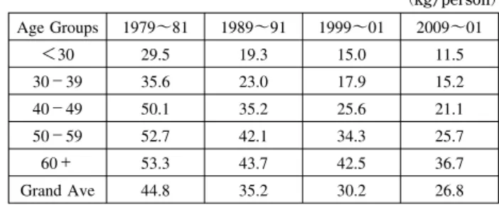
Starting in 1979, the FIES annual report publishes household purchases (consumption) of various goods and services classified by the age groups of household head (HH). Table 1 provides changes in per person2）

at-home rice consumption (＝raw rice to be prepared at-home, to repeat) during the past 30 years since 1980, classified by the HH age groups. Per person consumption on the grand av-erage (of approximately 8000 households3）_{) steadily decreased from 44.8 kg in 1980 (3 year simple}

averages of 1979 to 1881) to 26.8 kg in 2010, or by 40.0%. Rice consumption varies by HH age : a

Table 1 Per capita At-home Rice Consumption by HH Age Groups, 1980-2010 （kg/person） Age Groups 1979∼81 1989∼91 1999∼01 2009∼01 ＜30 29.5 19.3 15.0 11.5 30−39 35.6 23.0 17.9 15.2 40−49 50.1 35.2 25.6 21.1 50−59 52.7 42.1 34.3 25.7 60＋ 53.3 43.7 42.5 36.7 Grand Ave 44.8 35.2 30.2 26.8

(3)

per person of households with a HH under 30 years of age decreased sharply from 29.5 to 11.5 kg--by 61.0% --whereas that of households with a HH over 60 years of age decreased from 53.3 to 36.7 kg--by 31.0% --over the same period, resulting in even greater disparities between the young and the old in per capita rice consumption at home.

1）“Eating out rates” (total number of eating-out divided by 3 times×days of survey) increased from 11.3% in 1965 to 18.9% in 1990 and slightly declined to 17.1% in 2000, and 18.1% in 2010, according to the

Na-tional Nutrition Survey, 1990, p.46 and 2000, p.44, and 2010, pp.80−91, etc.

2）The ordinary households of 4 persons in size, for example, comprises the household head and his/her spouse of the similar age and two children of different age groups, who may eat more or much less foods than their parents.

3）Single person households are not included.

2. Deriving Individual Consumption of Family Members by Age

When household consumption classified by the age of household head (HH, again) is available, it may be straightforward to estimate individual consumption by age (of HH) by dividing total house-hold consumption by the number of persons contained in the househouse-hold, as was done in the previ-ous section. This approach could be valid, when one can assume that all members of the family eat nearly the same amount of foods in question as the household head, but this would seldom hold true in everyday lives. In the case of a 4-member family of HH aged 30, for example, 2 members are likely to be small children, who eat substantially less rice than their parents. Dividing total household consumption by 4 would result in substantial underestimates of individual consumption by adult members of the family of HH 30 years of age. In another case of a 4-member family of HH 45 years of age, the children are likely to be both high-teenagers, who normally eat substantially more rice than their parents. A simple division approach is likely to result in more than admissible overestimates of individual consumption by those in their mid-forties.

Mori and Inaba (1997) explicitly incorporated age structures of households classified by HH age groups into a (behavioral) equation system (Prais, 1953 ; Morishima, 1984) to estimate individual consumption by household members by age groups, with a few constraints of plausible assumptions, such as that individual consumption in the mid-forties should be equal to that in the early fifties, for example. Tanaka, Mori, and Inaba refined the model statistically later, replacing the equality con-straints by the more natural concon-straints of “gradual changes between successive age groups”4）_in

in-dividual consumption (Tanaka, Mori, and Inaba, 2004).

The Tanaka, Mori, and Inaba (TMI) model is summarized as below : Hj−∑CijXi＝Ej （i＝1−16 ; j＝1−10）（1）

Xk−Xk＋1＝Ek （k＝1−15）（2）

(4)

Hj: consumption by household headed by someone j years of age

Cij: number of individuals of i years of age in household headed by someone j years of age

Xi: estimated consumption by individuals of i years of age

Ej, Ek: residuals

Xi, individual consumption by i years of age, is estimated by minimizing the sum of squared

residu-als（1）and（2）above.

Table 2 provides estimates of individual annual at-home consumption of (raw) rice by 5 year age bracket up to the oldest category, 75＋years of age, for the period of 1980−2014. The two youngest groups, 0−4 and 5−9 years of age, do not represent any sizable segments of household age struc-tures classified by HH age groups. Judging from t values, etc., the consumption estimates for these age groups are not as stable as the older ones and not provided in Table 2.

A brief comparison of these data derived on individual consumption by age of household mem-bers by the TMI model in Table 2 to the data for household consumption by HH age groups simply divided by the household size in Table 1 confirms the discussion in the preceding section : older people in their 50s and 60s consume appreciably more rice than the younger ones in their 20s and 30s ; further-more, the younger generations (birth cohorts) seem to consume appreciably less (home-cooked) rice than the older ones.

4）Certain disparities are explicitly assumed between the youngest age groups : between 0−4 and 5−9, and 5 −9 and 10−14 years old, based on the nutrient intakes data, the National Nutrition Survey, various issues.

3. Decomposing Cohort Table into Age, Period, and Cohort Effects

When the general cohort table, comprising 12 age groups from the high-teenage years, 15−19, to the elderly years, 70−74, is decomposed into age/period/cohort effects by means of the Nakamura’s Bayesian cohort model (Nakamura, 1986), subject to the usual sum to zero constraints, we come up with the statistical results shown in Table 3. The three youngest age groups of 0−4, 5−9, and 10−14 years old are deleted, on the unproven premise that the eating habits of foods in general are firmly formed in the late teenage years (Ohga, 1999 ; Mori and Saegusa, 2010). The cells of the oldest age group, 75 and older, are also deleted, because they contain more than one age group, 75−79, conse-quently more than one birth cohort in each cell. The age cell, over 75 in 1980, for example, contains the cohort born in 1901 to 1905, the cohort born in 1896 to 1900, and so on, whereas the age cell of 70−74 years old in 1980 contains only one cohort, born in 1906 to 1910.

(5)

(6)

tool (Nakamura, 1986), with several technical modifications, as needed (Mori, Saegusa, and Dyck, 2012 ; Mori, Saegusa, and Inaba, 2014 ; etc.).

The basic structure of the model is summarized below :

In the ordinary cohort modeling, Xit, the action by i year-olds at the period t, is commonly

ex-pressed as follows, which may be “a poor approximation of how social change occurs” (Yang et al., 2008, p.1733), without any deductive theories like utility maximization in microeconomics, for exam-ple.

Xit＝B ＋Ai＋Pt＋Ck＋εit （3）

where :

Xit: event (average consumption) by i year-olds at the time, t

B: grand mean effect

Ai: the effect to be attributed to age, i years old

Pt: the effect to be attributed to period, t

Ck: the effect to be attributed to (birth) cohort (k)

εit: random errors

To center the parameters, we set the usual sum to zero constraints. ∑iAi＝∑tPt＝∑kCk＝０（4）

The model（3）can be written in the conventional matrix form of a least-squares regression below.

Y ＝Xb＋ε （5）

∑

i ∑t［X

it−（B ＋Ai＋Pt＋Ck）］2＝min! （6）

To overcome, or tackle with the identification problem stated above, one of the easiest measures taken by the conventional generalized models is to impose equality constraints on neighboring age and/or period groups (Yang, Fu, and Land, 2004, p.81). Nakamura imposes intuitively more natural assumptions of “gradual changes between successive parameters” for all three factors of age, period, and cohort effects and minimizes the following equation, allotting the hyper-parameters determined on the objective principle of ABIC (Akaike’s Bayesian Information Criterion) minimization.

1 σ2

A

∑（Ai−Ai＋1）2＋

1 σ2 P ∑（Pt−Pt＋1）2＋ 1 σ2 C ∑（Ck−Ck＋1）2＝min! （7）

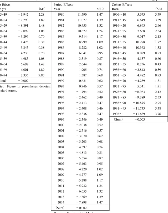
Table 3 demonstrates that age effects on rice consumption of individual consumers in their 50s, 60s, and the early 70s are distinctly positive, whereas age effects of younger adults under 40 years of age are clearly negative (under the sum to zero constraints,（4）above). Cohort effects are dis-tinctly positive for the older generations born before the mid-1950s, while for those born after the mid-1950s, cohort effects are increasingly negative, as large as −11.0kg, against the grand mean ef-fect of 36.1kg for those born after the mid-1980s, for example. The period efef-fects, provided in the middle column, suggest that individual rice consumption, after the age and cohort effects accounted for, has been steadily declining from the outset of the earlier 1980s.5）_{The period effects thus}

deter-mined could reflect changes in prices and household income, and other unknown forces, including unspecified “structural changes”(Huang and Bouis, 2001 ; Mori, 2015 ; etc.).

(7)

co-Table 3 Individual At-home Rice Cosumption by Age Decomposed into Age, Period, and Cohort Effects, 1980-2014, Bayesian Model

Grand Mean Effects＝36.081（.151）（kg/person）

Age Efects

Age yrs （SE）

Period Effects Year （SE） Cohort Effects Born （SE） 15−19 −1.942 2.28 1980 11.590 1.47 1906∼10 5.673 3.79 20−24 −7.290 1.89 1981 11.027 1.39 1911∼15 6.649 3.39 25−29 −8.891 1.48 1982 10.453 1.32 1916∼20 6.863 2.96 30−34 −7.099 1.08 1983 10.622 1.24 1921∼25 7.668 2.54 35−39 −3.296 0.70 1984 9.514 1.17 1926∼30 9.017 2.13 40−44 1.426 0.38 1985 8.999 1.09 1931∼35 10.298 1.72 45−49 3.845 0.38 1986 8.282 1.02 1936∼40 10.362 1.32 50−54 4.233 0.70 1987 6.041 0.95 1941∼45 8.089 0.93 55−59 4.983 1.08 1988 3.319 0.87 1946∼50 4.137 0.60 60−64 5.692 1.48 1989 2.644 0.81 1951∼55 −0.236 0.43 65−69 6.001 1.89 1990 1.905 0.74 1956∼60 −3.842 0.59 70−74 2.336 9.83 1991 1.387 0.68 1961∼65 −4.482 0.93 （Sum） −0.002 1992 0.621 0.62 1966∼70 −4.239 1.31

(8)

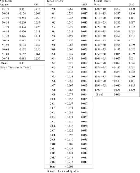
Table 4 Individual At-home Rice Consumption by Age Decomposed into Age, Period, and Cohort Effects in Logs, 1980-2014, Bayesian Model

Grand Mean Effects＝3.45（.004）（in natural logs）

Age Efects

Age yrs （SE）

Period Effects Year （SE） Cohort Effects Born （SE） 15−19 0.081 0.078 1980 0.267 0.049 1906∼10 0.212 0.130 20−24 −0.174 0.064 1981 0.256 0.047 1911∼15 0.237 0.116 25−29 −0.263 0.050 1982 0.243 0.044 1916∼20 0.246 0.101 30−34 −0.209 0.037 1983 0.240 0.042 1921∼25 0.282 0.087 35−39 −0.094 0.023 1984 0.225 0.039 1926∼30 0.325 0.072 40−44 0.026 0.011 1985 0.211 0.036 1931∼35 0.361 0.058 45−49 0.076 0.011 1986 0.199 0.034 1936∼40 0.367 0.044 50−54 0.082 0.023 1987 0.150 0.031 1941∼45 0.331 0.031 55−59 0.104 0.037 1988 0.088 0.028 1946∼50 0.258 0.019 60−64 0.132 0.050 1989 0.066 0.026 1951∼55 0.152 0.012 65−69 0.152 0.064 1990 0.049 0.023 1956∼60 0.035 0.019 70−74 0.088 0.336 1991 0.041 0.021 1961∼65 −0.027 0.031 （Sum） 0.001 1992 0.028 0.019 1966∼70 −0.067 0.044

Note : The same as Table 3. 1993 0.025 0.017 1971∼75 −0.147 0.058

1994 −0.047 0.015 1976∼80 −0.273 0.072 1995 −0.058 0.014 1981∼85 −0.448 0.086 1996 −0.056 0.013 1986∼90 −0.583 0.101 1997 −0.062 0.013 1991∼95 −0.640 0.115 1998 −0.062 0.013 1996∼ −0.621 0.129 1999 −0.077 0.014 （Sum） 0.000 2000 −0.052 0.015 2001 −0.057 0.017 2002 −0.071 0.019 2003 −0.081 0.021 2004 −0.111 0.023 2005 −0.120 0.026 2006 −0.132 0.028 2007 −0.122 0.031 2008 −0.095 0.034 2009 −0.110 0.036 2010 −0.108 0.039 2011 −0.127 0.042 2012 −0.151 0.044 2013 −0.177 0.047 2014 −0.213 0.049 （Sum） −0.001

(9)

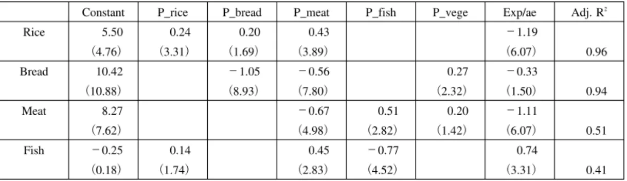
hort table, Table 2, is decomposed in natural logs to produce Table 4, which is essentially the same as Table 3. The age effects are clearly positive for the older age groups and the newer generations are shown to carry steadily declining cohort effects, so forth. The period effects provided in Table 4, estimated in natural logs are regressed against the prices of rice, bread, fish, meat, and vegetables and household living expenditures per adult equivalence scale as a proxy for income (OECD, 1982), all deflated by the CPI for all goods and services, resulting in equation（8）. The own price elasticity of rice at 0.24 does not seem economically reasonable ; cross-price elasticities of bread and meat are 0.38 and 0.64, respectively ; those of fish and vegetables, both of which carry negative signs should be neglected because the coefficients lack statistical significance ; income elasticity at −0.95 may or may not be reasonable but should not be neglected.

（gm＋pe）＝4.90＋0.24ln（p-rice）＋0.38ln（p-bread）＋0.64ln（p-meat）−0.38ln（p-fish）

（4.53）（3.69）（2.69）（4.96）（2.12）

−0.23（p-vege）−0.95ln（ex/ae）（8）

（1.27）（4.55） Adj.R2_＝0.97

When prices of fish and vegetables are deleted, we come up with the similar outcomes, as shown below in（9）.

（gm＋pe）＝5.50＋0.24ln（p-rice）＋0.20ln（p-bread）＋0.43ln（p-meat）−1.19ln（ex/ae）（9）

（4.76）（3.31）（1.69）（3.88）（6.07） Adj.R2_＝0.96

Figures in parentheses in the equations above denote t values.

Considering that a drastic decline in at-home rice consumption in the past half century may have been affected by unidentified factors other than the economic variables of prices and income and the demographic effects, we may need further exploration for changes in rice consumption.

Tables 5, 6, and 76）_{provide the cohort parameters in logs for at-home bread, meat and fish}

con-sumption, respectively, estimated in the same fashions as for rice presented in Table 4. The period effects for consumption of bread, meat, and fish, respectively for 35 years from 1980 to 2014 are re-gressed against prices of four or five presumably related products, rice, bread, meat, fish, and vege-tables and per adult household expenditures, as conducted for rice above. Table 8 summarizes the economic demand elasticities for rice, bread, meat, and fish, estimated in this “two-step approach” : first to identify period effects from 1980 to 2014, controlling for age and cohort effects, and then to regress the period effects (＋ grand mean effect) for the specific product against the prices of re-lated products and household incomes.

To repeat, the own price elasticity of rice is estimated at ＋0.24, while the cross price elasticities of bread and meat are estimated at ＋0.20 and ＋0.43, respectively with reasonable statistical signifi-cance and (per adult household) expenditure elasticity at −1.19 with high t-value, with the model adjusted R2 _{at 0.96. Intuitively, the positive own price elasticity along with a very high negative}

(10)

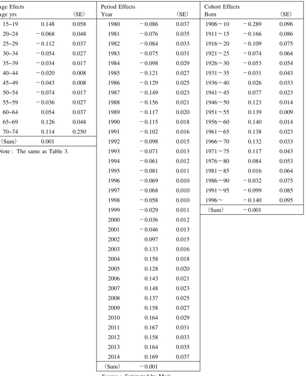
Table 5 Individual At-home Bread Consumption by Age Decomposed into Age, Period, and Cohort Effects in Logs, 1980-2014, Bayesian Model

Age Efects

Age yrs （SE）

Period Effects Year （SE） Cohort Effects Born （SE） 15−19 0.148 0.058 1980 −0.086 0.037 1906∼10 −0.289 0.096 20−24 −0.068 0.048 1981 −0.076 0.035 1911∼15 −0.166 0.086 25−29 −0.112 0.037 1982 −0.084 0.033 1916∼20 −0.109 0.075 30−34 −0.054 0.027 1983 −0.075 0.031 1921∼25 −0.074 0.064 35−39 −0.034 0.017 1984 −0.098 0.029 1926∼30 −0.053 0.054 40−44 −0.020 0.008 1985 −0.121 0.027 1931∼35 −0.031 0.043 45−49 −0.043 0.008 1986 −0.129 0.025 1936∼40 0.026 0.033 50−54 −0.074 0.017 1987 −0.149 0.023 1941∼45 0.077 0.023 55−59 −0.036 0.027 1988 −0.156 0.021 1946∼50 0.123 0.014 60−64 0.054 0.037 1989 −0.117 0.020 1951∼55 0.139 0.009 65−69 0.126 0.048 1990 −0.115 0.018 1956∼60 0.140 0.014 70−74 0.114 0.250 1991 −0.102 0.016 1961∼65 0.138 0.023 （Sum） 0.001 1992 −0.098 0.015 1966∼70 0.132 0.033

Note : The same as Table 3. 1993 −0.071 0.013 1971∼75 0.117 0.043

(11)

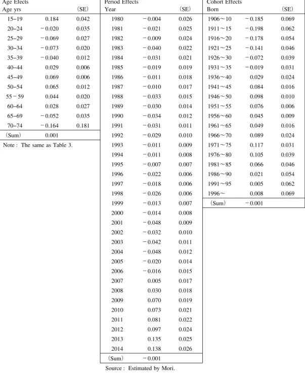
Table 6 Individual At-home Meat Consumption by Age Decomposed into Age, Period, and Cohort Effects in Logs, 1980-2014, Bayesian Model

Age Efects

Age yrs （SE）

Period Effects Year （SE） Cohort Effects Born （SE） 15−19 0.184 0.042 1980 −0.004 0.026 1906∼10 −0.185 0.069 20−24 −0.020 0.035 1981 −0.021 0.025 1911∼15 −0.198 0.062 25−29 −0.069 0.027 1982 −0.009 0.024 1916∼20 −0.178 0.054 30−34 −0.073 0.020 1983 −0.040 0.022 1921∼25 −0.141 0.046 35−39 −0.040 0.012 1984 −0.031 0.021 1926∼30 −0.072 0.039 40−44 0.029 0.006 1985 −0.019 0.019 1931∼35 −0.019 0.031 45−49 0.069 0.006 1986 −0.011 0.018 1936∼40 0.029 0.024 50−54 0.065 0.012 1987 −0.010 0.017 1941∼45 0.084 0.016 55−59 0.044 0.020 1988 −0.033 0.015 1946∼50 0.098 0.010 60−64 0.028 0.027 1989 −0.030 0.014 1951∼55 0.076 0.006 65−69 −0.052 0.035 1990 −0.034 0.012 1956∼60 0.045 0.009 70−74 −0.164 0.181 1991 −0.031 0.011 1961∼65 0.049 0.016 （Sum） 0.001 1992 −0.029 0.010 1966∼70 0.089 0.024

Note : The same as Table 3. 1993 −0.011 0.009 1971∼75 0.117 0.031

(12)

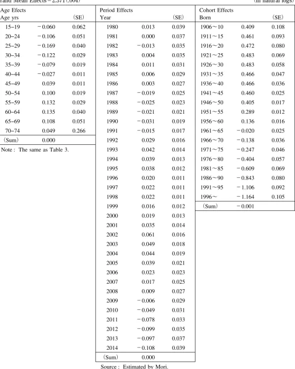
Table 7 Individual At-home Fish Consumption by Age Decomposed into Age, Period, and Cohort Effects in Logs, 1980-2014, Bayesian Model

Age Efects

Age yrs （SE）

Period Effects Year （SE） Cohort Effects Born （SE） 15−19 −0.060 0.062 1980 0.013 0.039 1906∼10 0.409 0.108 20−24 −0.106 0.051 1981 0.000 0.037 1911∼15 0.461 0.093 25−29 −0.169 0.040 1982 −0.013 0.035 1916∼20 0.472 0.080 30−34 −0.122 0.029 1983 0.004 0.035 1921∼25 0.483 0.069 35−39 −0.079 0.019 1984 0.011 0.031 1926∼30 0.483 0.058 40−44 −0.027 0.011 1985 0.006 0.029 1931∼35 0.466 0.047 45−49 0.039 0.011 1986 0.003 0.027 1936∼40 0.466 0.036 50−54 0.100 0.019 1987 −0.019 0.025 1941∼45 0.460 0.025 55−59 0.132 0.029 1988 −0.025 0.023 1946∼50 0.405 0.017 60−64 0.135 0.040 1989 −0.021 0.021 1951∼55 0.289 0.012 65−69 0.108 0.051 1990 −0.031 0.019 1956∼60 0.136 0.016 70−74 0.049 0.266 1991 −0.015 0.017 1961∼65 −0.020 0.025 （Sum） 0.000 1992 0.029 0.016 1966∼70 −0.138 0.036

Note : The same as Table 3. 1993 0.042 0.014 1971∼75 −0.247 0.046

1994 0.039 0.013 1976∼80 −0.404 0.057 1995 0.038 0.012 1981∼85 −0.609 0.069 1996 0.020 0.011 1986∼90 −0.843 0.080 1997 0.022 0.011 1991∼95 −1.106 0.092 1998 0.022 0.011 1996∼ −1.164 0.105 1999 0.016 0.012 （Sum） −0.001 2000 0.019 0.013 2001 0.035 0.014 2002 0.061 0.016 2003 0.049 0.018 2004 0.044 0.019 2005 0.039 0.021 2006 0.023 0.023 2007 0.017 0.025 2008 0.009 0.027 2009 −0.006 0.029 2010 −0.049 0.031 2011 −0.078 0.033 2012 −0.099 0.035 2013 −0.097 0.037 2014 −0.108 0.039 （Sum） 0.000

(13)

fish.

5）The authors also decomposed the same cohort table, Table 2, by means of the “intrinsic estimator” (IE) developed by Yang et al. (2004 and 2008), to produce cohort parameters very similar to those estimated by the Nakamura’s Bayesian model. The IE results are provided in Appendix Table 1.

6）Cohort tables comprising individual consumption by age groups for 35 years from 1980 to 2014 for bread, meat, and fish are provided in Appendix Tables 2, 3, and 4.

4. Determining Cohort Parameters and Economic Demand Elasticities in One

-Step by Augmented Cohort Models

In micro-economics, demand for a chosen product is determined by its own price and prices of other related products and by the incomes of those who demand the product and more often than not by changes in social circumstances, such as increases in health-consciousness (B-W Lin et al., 2003), “westernization” in diet (Tokoyama and Egaitsu, 1994), etc. R. Schrimper raised a question on Salathe’s presentation at the American Agricultural Association Meeting, 1979, “The Effect of Changes in Population Characteristics on Food Consumption” (Salathe, 1979), asking that “is it rea-sonable to expect all generations to follow the same transformation of eating habits over the life cy-cle?” He suggested that “cohort effects as opposed to pure age effects” should not be overlooked (Schrimper, 1979, p. 1059). Stimulated by his insightful comments, we have been trying to incorpo-rate age/cohort effects into food demand analyses for some time since the early 2000s (Mori eds., 2001).

If one’s consumption of a certain food is determined explicitly by the economic factors such as prices and incomes on top of demographic factors of age/cohort effects, it should be theoretically desirable to determine the impacts of economic and demographic variables simultaneously in one-step. This is what Stewart and Blisard proposed (2008) and Saegusa et al. have been following suits

Table 8 Demand Elasticities Summary, Rice, Bread, Meat, and Fish, Using Period Effects Identified by Bayesian Cohort Analysis

Constant P_rice P_bread P_meat P_fish P_vege Exp/ae Adj. R2

Rice 5.50 0.24 0.20 0.43 −1.19 （4.76）（3.31）（1.69）（3.89）（6.07） 0.96 Bread 10.42 −1.05 −0.56 0.27 −0.33 （10.88）（8.93）（7.80）（2.32）（1.50） 0.94 Meat 8.27 −0.67 0.51 0.20 −1.11 （7.62）（4.98）（2.82）（1.42）（6.07） 0.51 Fish −0.25 0.14 0.45 −0.77 0.74 （0.18）（1.74）（2.83）（4.52）（3.31） 0.41

Notes : All prices and expenditures deflated by CPI（2010＝100）; figures in parentheses denote t-values. The prices which showed t-values smaller than 1 in absolute value not used.

(14)

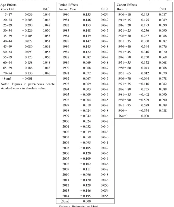
Table 9 At-home Rice Consumption by Age Decomposed into Age/Period/Cohort Effects, 1980-2014 Augmented BE Model in Logs

Own Price Elasticity of Rice＝.01（.12）

Cross Price Elasticity of Bread＝.16（.23）; Cross Price Elasticity of Meat＝.34（.23） Cross Price Elasticity of Fish＝−.30（.25）; Income Elasticity＝−.72（.41）

Grand Mean Effect＝6.061（2.437） ABIC＝−1120.921 （in natural logs）

Age Effects

Years Old （SE）

Period Effects

Annual Year （SE）

Cohort Effects Born in （SE） 15−17 0.039 0.046 1980 0.155 0.054 1906∼10 0.145 0.087 20−24 −0.208 0.046 1981 0.146 0.049 1911∼15 0.175 0.089 25−29 −0.290 0.048 1982 0.153 0.048 1916∼20 0.193 0.090 30−34 −0.229 0.050 1983 0.148 0.047 1921∼25 0.236 0.090 35−39 −0.105 0.055 1984 0.139 0.047 1926∼30 0.287 0.088 40−44 0.022 0.061 1985 0.142 0.049 1931∼35 0.330 0.082 45−49 0.080 0.061 1986 0.145 0.048 1936∼40 0.344 0.076 50−54 0.093 0.055 1987 0.122 0.049 1941∼45 0.316 0.070 55−59 0.123 0.050 1988 0.082 0.047 1946∼50 0.250 0.068 60−64 0.158 0.048 1989 0.069 0.048 1951∼55 0.152 0.068 65−69 0.186 0.046 1990 0.068 0.047 1956∼60 0.043 0.068 70−74 0.130 0.046 1991 0.072 0.048 1961∼65 −0.012 0.070 （Sum） −0.001 1992 0.067 0.047 1966∼70 −0.044 0.078

Note : Figures in parentheses denote standard errors in absolute value.

1993 0.069 0.044 1971∼75 −0.116 0.082 1994 0.003 0.047 1976∼80 −0.235 0.088 1995 −0.009 0.046 1981∼85 −0.402 0.090 1996 −0.004 0.045 1986∼90 −0.529 0.090 1997 −0.019 0.047 1991∼95 −0.579 0.089 1998 −0.024 0.048 1996∼ −0.554 0.088 1999 −0.042 0.046 （Sum） 0.000 2000 −0.024 0.042 2001 −0.032 0.040 2002 −0.039 0.043 2003 −0.059 0.040 2004 −0.095 0.041 2005 −0.105 0.042 2006 −0.120 0.045 2007 −0.109 0.046 2008 −0.102 0.046 2009 −0.111 0.048 2010 −0.096 0.048 2011 −0.120 0.046 2012 −0.129 0.050 2013 −0.146 0.054 2014 −0.195 0.055 （Sum） 0.000

(15)

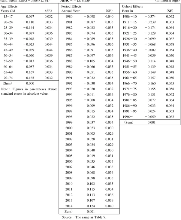
Table 10 At-home Bread Consumption by Age Decomposed into Age/Period/Cohort Effects, 1980-2014 Augmented BE Model in Logs

Own Price Elasticity of Bread＝−0.97（.17）

Cross Price Elasticity of Rice＝.07（.09）; Cross Price Elasticity of Meat＝．13（．17） Cross Price Elasticity of Fish＝−.15（.18）; Income Elasticity＝.15（.30）

Age Effects

Years Old （SE）

Period Effects

Cohort Effects Born in （SE） 15−17 0.097 0.032 1980 −0.098 0.040 1906∼10 −0.374 0.062 20−24 −0.110 0.033 1981 −0.087 0.035 1911∼15 −0.239 0.063 25−29 −0.144 0.034 1982 −0.083 0.035 1916∼20 −0.174 0.064 30−34 −0.077 0.036 1983 −0.074 0.035 1921∼25 −0.129 0.064 35−39 −0.048 0.039 1984 −0.089 0.035 1926∼30 −0.099 0.062 40−44 −0.025 0.044 1985 −0.096 0.036 1931∼35 −0.068 0.058 45−49 −0.039 0.044 1986 −0.091 0.035 1936∼40 −0.002 0.054 50−54 −0.060 0.039 1987 −0.097 0.036 1941∼45 0.059 0.050 55−59 −0.013 0.036 1988 −0.105 0.034 1946∼50 0.114 0.048 60−64 0.087 0.034 1989 −0.066 0.035 1951∼55 0.139 0.048 65−69 0.167 0.033 1990 −0.051 0.035 1956∼60 0.149 0.048 70−74 0.165 0.032 1991 −0.032 0.035 1961∼65 0.157 0.050 （Sum） 0.000 1992 −0.030 0.034 1966∼70 0.160 0.055

1993 −0.020 0.032 1971∼75 0.155 0.058 1994 −0.011 0.034 1976∼80 0.131 0.062 1995 −0.008 0.034 1981∼85 0.072 0.064 1996 0.009 0.032 1986∼90 0.033 0.064 1997 0.015 0.034 1991∼95 −0.024 0.063 1998 0.022 0.035 1996∼ −0.059 0.062 1999 0.037 0.034 （Sum） 0.001 2000 0.023 0.030 2001 0.003 0.029 2002 0.028 0.031 2003 0.034 0.029 2004 0.040 0.030 2005 0.019 0.031 2006 0.035 0.033 2007 0.046 0.033 2008 0.068 0.034 2009 0.098 0.035 2010 0.103 0.035 2011 0.115 0.034 2012 0.113 0.036 2013 0.107 0.039 2014 0.124 0.040 （Sum） 0.001

(16)

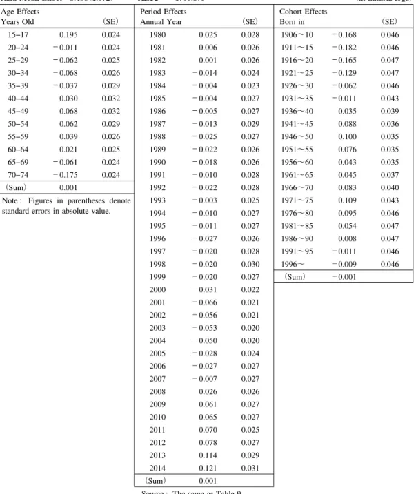
Table 11 At-home Meat Consumption by Age Decomposed into Age/Period/Cohort Effects, 1980-2014 Augmented BE Model in Logs

Own Price Elasticity of Meat＝−.22（.14）

Cross Price Elasticity of Fish＝.22（.16）; Cross Price Elasticity of Bread＝−.11（.15） Cross Price Elasticity of Veges＝−.15（.07）; Income Elasticity＝.05（.26）

Age Effects

Years Old （SE）

Period Effects

Cohort Effects Born in （SE） 15−17 0.195 0.024 1980 0.025 0.028 1906∼10 −0.168 0.046 20−24 −0.011 0.024 1981 0.006 0.026 1911∼15 −0.182 0.046 25−29 −0.062 0.025 1982 0.001 0.026 1916∼20 −0.165 0.047 30−34 −0.068 0.026 1983 −0.014 0.024 1921∼25 −0.129 0.047 35−39 −0.037 0.029 1984 −0.004 0.023 1926∼30 −0.062 0.046 40−44 0.030 0.032 1985 −0.004 0.027 1931∼35 −0.011 0.043 45−49 0.068 0.032 1986 −0.005 0.027 1936∼40 0.035 0.039 50−54 0.062 0.029 1987 −0.013 0.029 1941∼45 0.088 0.036 55−59 0.039 0.026 1988 −0.025 0.027 1946∼50 0.100 0.035 60−64 0.021 0.025 1989 −0.022 0.026 1951∼55 0.076 0.035 65−69 −0.061 0.024 1990 −0.018 0.026 1956∼60 0.043 0.035 70−74 −0.175 0.024 1991 −0.010 0.028 1961∼65 0.045 0.037 （Sum） 0.001 1992 −0.022 0.028 1966∼70 0.083 0.040

1993 −0.003 0.025 1971∼75 0.109 0.043 1994 −0.010 0.027 1976∼80 0.095 0.046 1995 −0.011 0.027 1981∼85 0.054 0.047 1996 −0.027 0.026 1986∼90 0.008 0.047 1997 −0.020 0.028 1991∼95 −0.011 0.046 1998 −0.020 0.030 1996∼ −0.009 0.046 1999 −0.020 0.027 （Sum） −0.001 2000 −0.031 0.022 2001 −0.066 0.021 2002 −0.056 0.021 2003 −0.053 0.020 2004 −0.050 0.020 2005 −0.028 0.024 2006 −0.027 0.027 2007 −0.007 0.027 2008 0.026 0.026 2009 0.061 0.027 2010 0.065 0.027 2011 0.070 0.025 2012 0.078 0.027 2013 0.114 0.029 2014 0.121 0.031 （Sum） 0.001

(17)

Table 12 At-home Fish Consumption by Age Decomposed into Age/Period/Cohort Effects, 1980-2014 Augmented BE Model in Logs

Own Price Elasticity of Fish＝−.64（.17）

Cross Price Elasticity of Meat＝.28（.16）; Cross Price Elasticity of Rice＝.02（.09） Cross Price Elasticity of Veges＝−.14（.09）; Income Elasticity＝.41（.30）

Age Effects

Years Old （SE）

Period Effects

Cohort Effects Born in （SE） 15−17 −0.040 0.036 1980 0.025 0.036 1906∼10 0.446 0.069 20−24 −0.089 0.036 1981 0.013 0.033 1911∼15 0.490 0.071 25−29 −0.156 0.038 1982 0.000 0.033 1916∼20 0.499 0.072 30−34 −0.113 0.040 1983 −0.001 0.032 1921∼25 0.505 0.072 35−39 −0.074 0.043 1984 −0.003 0.032 1926∼30 0.502 0.070 40−44 −0.025 0.048 1985 0.000 0.033 1931∼35 0.481 0.067 45−49 0.038 0.048 1986 0.004 0.033 1936∼40 0.476 0.062 50−54 0.094 0.043 1987 0.000 0.033 1941∼45 0.467 0.056 55−59 0.123 0.040 1988 −0.006 0.032 1946∼50 0.408 0.054 60−64 0.122 0.038 1989 0.000 0.032 1951∼55 0.289 0.054 65−69 0.091 0.036 1990 0.007 0.032 1956∼60 0.132 0.054 70−74 0.028 0.036 1991 0.025 0.032 1961∼65 −0.027 0.056 （Sum） −0.001 1992 0.048 0.032 1966∼70 −0.150 0.064

1993 0.052 0.031 1971∼75 −0.262 0.066 1994 0.047 0.032 1976∼80 −0.422 0.071 1995 0.045 0.032 1981∼85 −0.632 0.072 1996 0.028 0.031 1986∼90 −0.870 0.072 1997 0.027 0.032 1991∼95 −1.137 0.071 1998 0.033 0.032 1996∼ −1.195 0.069 1999 0.026 0.031 （Sum） 0.000 2000 0.021 0.029 2001 0.031 0.028 2002 0.038 0.029 2003 0.017 0.028 2004 0.000 0.028 2005 −0.008 0.026 2006 −0.010 0.026 2007 −0.018 0.028 2008 −0.031 0.029 2009 −0.042 0.030 2010 −0.061 0.031 2011 −0.076 0.031 2012 −0.084 0.033 2013 −0.076 0.036 2014 −0.072 0.037 （Sum） −0.001

(18)

(Saegusa and Mori, 2012 ; Mori, Saegusa, and Dyck, 2012 ; Mori, Saegusa, and Tanaka, 2015 ; etc.). Saegusa named this one-step approach “augmented cohort model” following the lead of Stewart and Blisard, 2008, p.48.

Tables 9, 10, 11, and 12 provide estimates of economic elasticities on top of traditional cohort pa-rameters--age, period, and cohort effects--for rice, bread, meat, and fish, respectively. We first intro-duced prices of all 5 products, rice, bread, meat, fish, and vegetables, irrespective of the product for analysis and selected the best-performing output for each product strictly in reference to ABIC of the model.

At first, one may notice that the structure of age/cohort effects remained basically, if not exactly, the same as the traditional cohort model without the economic variables incorporated. The aug-mented model has resulted in changes in period effects, as expected, for all cases of rice, bread, meat, and fish : generally flatter than the traditional model but not totally flat, implying that there remain unknown other factors which may have affected long-run changes in at-home consumption of all four products for the past some 30 years since 1980 : the case for rice is graphically pre-sented in Figure 1. Table 13 summarizes the key economic parameters determined by the aug-mented model shown in the upper parts of Tables 9, 10, 11, and 12, respectively.

The own price elasticity of rice is estimated at ＋0.01, not significantly different from zero, whereas that for bread, meat and fish is estimated at −0.97, −0.22, and −0.64, respectively, all sig-nificantly different from zero. Meat and fish are found mutually competitive, with cross price elastic-ity of fish on meat is estimated at 0.22, and that of meat on fish at 0.28, both statistically different from zero at 5% level. In respect of expenditure elasticity, rice is estimated at −0.72 (SE＝0.41) and fish at 0.41 (SE＝0.30) and neither bread nor meat found different from zero statistically. Intuitively, estimates of demand elasticities shown in Table 13 appear to be more reasonable than those pro-vided in linear regression models（8）and（9）in the previous section.

(19)

20.00 25.00 30.00 35.00 40.00 45.00 50.00 19 80 19 82 19 84 19 86 19 88 19 90 19 92 19 94 19 96 19 98 20 00 20 02 20 04 20 06 20 08 20 10 20 12 20 14 k g / p e r s o n Year cap_Q APC_PE Aug_PE

Figure 1 Comparison of Simple Average with Age_Cohort Effects Compensated, and Age_Cohort and Economic Factors Compensated Period Effects,

At-home Rice Consumption, 1980-2014

Table 13 Demand Elasticities for Rice, Bread, Meat, and Fish, Estimated by Augmented Bayesian Model

P_rice P_bread P_meat P_fish P_veges Exp/ae ABIC

Rice 0.01 0.16 0.34 −0.30 −0.72 （0.12）（0.23）（0.23）（0.25）（0.41） −1120.92 Bread 0.07 −0.97 0.13 −0.15 0.15 （0.09）（0.17）（0.17）（0.18）（0.30） −1378.559 Meat −0.11 −0.22 0.22 −0.15 0.05 （0.15）（0.14）（0.16）（0.07）（0.26） −1736.379 Fish 0.02 0.28 −0.64 −0.14 0.41 （0.09）（0.16）（0.17）（0.09）（0.30） −1153.064

Notes : All prices and expenditures deflated by CPI（2010＝100）;

figures in parentheses denote standard errors of estimates in absolute values.

(20)

The same appears to be the case with fish, where the older people consume distinctly more fish than the younger ones, by referring to Table 12 and Appendix Table 7.

Demand elasticities of rice, bread, meat and fish estimated by the augmented model-T are sum-marized in Table 14. The own price elasticities for all four products, rice, bread, meat and fish are estimated with theoretically valid sign, at −0.15, −0.92, −0.16, and −0.65, respectively. In respect to cross-relationship, rice and meat are found statistically competitive with bread, at ＋0.17 and ＋ 0.33, respectively, fish is competitive to meat, with the cross price elasticity of fish at ＋0.21, so forth. The expenditure elasticity of fish is estimated at ＋0.53, whereas that of rice at −0.35 and those of bread and meat are found not significantly different from zero. Trend is found statistically negative on changes in at-home consumption of both rice and fish and the opposite is the case with bread and meat.

Saegusa applied T, a straight trend, which is 10 for 1980, 11 for 1981, −−, 44 for 2014, as men-tioned above, without any theoretical and/or empirical background supporting it. We are not certain if it can be extrapolated to the year 2020 as 50, for example. For the sake of statistical fitness, it would be possible to apply kinky time trend, which is 10 for the first 11 years from 1980 to 1990, and then 11 for 1991, 12 for 1992, −−, 34 for 2014, for example. There may be some empirical justifi-cation for this modifijustifi-cation, since Japan’s economy plunged into a long period of slow growth after the bubble burst in 1991. Tedious experiments along this line may or may not produce some useful insights into the nature of long-run changes in at-home rice consumption.

5. Demand System Analyses Using Period Effects Estimated by the

Tradi-tional A/P/C Bayesian Model

As shown clearly by Table 16, nearly 50% of daily energy intake of 2,291 kilo calories (kc) de-pended on rice and 10.9% on wheat, respectively and meat, eggs and milk and dairy products com-bined accounted for 3.9% and fish 3.8%, respectively in 1960. The dependence on rice then

de-Table 14 Demand Elasticities for Rice, Bread, Meat, and Fish, Estimated by Augmented Bayesian Model, with Time Trend

P_rice P_bread P_meat P_fish P_veges Exp/ae Trend ABIC

Rice −0.15 0.13 0.03 −0.32 −0.35 −0.023 （0.11）（0.19）（0.21）（0.21）（0.36）（0.006） −1134.93 Bread 0.17 −0.92 0.33 −0.15 −0.10 0.014 （0.09）（0.15）（0.16）（0.16）（0.28）（0.004） −1388.566 Meat −0.11 −0.16 0.21 −0.15 0.00 0.004 （0.14）（0.15）（0.15）（0.07）（0.26）（0.004） −1739.796 Fish 0.17 −0.65 −0.13 0.53 −0.009 （0.16）（0.16）（0.09）（0.27）（0.004） −1157.662 Notes : All prices and expenditures deflated by CPI（2010＝100）;

figures in parentheses denote standard errors of estimates in absolute values.

(21)

Table 15 At-home Rice Consumption by Age Decomposed into Age/Period/Cohort Effects, 1980-2014 Augmented BE Model-T in Logs

Own Price Elasticity of Rice＝−.15（.11）; Trend Effect＝−.023（.006） Cross Price Elasticity of Bread＝.13（.23）; Cross Price Elasticity of Meat＝.03（.21）

Cross Price Elasticity of Fish＝−.32（.21）; Income Elasticity＝−.35（.36）

Age Effects

Years Old （SE）

Period Effects

Cohort Effects Born in （SE） 15−17 −0.126 0.047 1980 0.012 0.044 1906∼10 −0.114 0.090 20−24 −0.344 0.048 1981 0.016 0.041 1911∼15 −0.065 0.092 25−29 −0.395 0.050 1982 0.030 0.041 1916∼20 −0.016 0.093 30−34 −0.303 0.052 1983 0.036 0.041 1921∼25 0.056 0.092 35−39 −0.150 0.057 1984 0.035 0.041 1926∼30 0.136 0.090 40−44 0.007 0.064 1985 0.043 0.041 1931∼35 0.210 0.084 45−49 0.095 0.064 1986 0.050 0.041 1936∼40 0.254 0.078 50−54 0.139 0.057 1987 0.034 0.042 1941∼45 0.255 0.072 55−59 0.198 0.052 1988 0.001 0.041 1946∼50 0.219 0.070 60−64 0.263 0.050 1989 −0.003 0.041 1951∼55 0.151 0.070 65−69 0.321 0.048 1990 0.005 0.041 1956∼60 0.073 0.070 70−74 0.294 0.047 1991 0.012 0.042 1961∼65 0.048 0.073 （Sum） −0.001 1992 0.013 0.043 1966∼70 0.045 0.080

(22)

creased steadily to 34.0% in 1975, 25.9% in 1990, and 23.7% in 2010, respectively, whereas that of wheat slightly increased to 12.6% in 1975 and 13.5% in 20107）_{. The percentage of meat, eggs and}

milk and dairy products in total caloric intakes conspicuously increased to 10.2% in 1975, 13.9% in 1990, and 15.9% in 2010 and that of fish increased moderately to 4.7% in 1975 and 5.4% in 1990 and then slightly declined to 4.5% in 2010.

As mentioned earlier, at-home rice consumption (preparation of raw rice at home) accounts for a declining percentage of total rice supply and yet remains the most important segment of total con-sumption today.

Recognizing the limitations, the demand system for this analysis comprises 4 commodity groups, rice, bread, (fresh) meat, and (fresh) fish. The Almost Ideal Demand System (AIDS) model, devel-oped by Deaton and Muellbauer (1980), is used and in this article a unique demand system ap-proach in association with the Bayesian A/P/C analysis is also proposed in Technical Supplement.

The expenditure share equation of commodity i is expressed as below w（i）＝αi＋βiln（y/P）＋∑γijln（pj）（10）

αi,βi, andγijare parameters to be estimated

w（i）: commodity i’s share in total expenditures for all the 4 commodities y : total expenditures for the 4 commodities

pj: real prices of commodity j

P : Stone’s price index

Based on the Slutsky equations, the restrictions below are normally imposed Table 1６ Changes in Energy Sources by Commodity Groups,

from 1960 to 2012

（％） FY1960 YF1975 YF1990 YF2010 YF2012

(23)

Adding up :∑4 i＝1α i＝1, 4 ∑ i＝1β i＝0, 4 ∑ i＝1γ ij＝0 （11） Homogeneity Condition：∑ j γ ij＝0 （12） Symmetry Assumptions：γij＝γji （13）

In order to calculate the expenditure for commodity i in year t, we use the period effect for i at t in kg, in place of simple per capita average consumption in the ordinary time-series analyses, multi-plied by the average real price of the commodity i in the year, t. The consumption data we use are thus per adult consumption, with age and cohort effects accounted for (as described in the preced-ing sections).

We tried AIDS estimation of demand elasticities with several modifications, with all the theoretical restrictions imposed, or one of them, symmetry deleted, for example, or trend imposed on rice, etc.

Table 17 Demand Elasticities for Rice, Bread, Meat, and Fish Estimated by AIDS Model, Using Period Effects,

with Age and Cohort Effects Accounted for, 1980-2014 a）

P_Rice P_Bread P_Meat P_Fish Expend.

Rice −0.57 −0.13 −0.15 −0.14 0.94 （0.015）（0.007）（0.012）（0.017）（0.017） Bread 0.29 −1.11 −0.16 0.17 1.07 （0.010）（0.008）（0.010）（0.011）（0.002） Meat −0.12 −0.07 −0.73 −0.10 1.02 （0.008）（0.004）（0.013）（0.016）（0.001） Fish −0.13 0.09 −0.12 −0.84 0.99 （0.014）（0.005）（0.020）（0.03）（0.001） b）

P_Rice P_Bread P_Meat P_Fish

Rice −0.49 −0.19 −0.59 −0.60

Bread −0.10 −0.72 0.20 −0.22

Meat −0.40 −0.06 −1.16 −0.27

Fish 0.12 0.11 0.60 −0.06

Notes : All prices and expenditures deflated by CPI（2010＝100）;

(24)

Table 17 provides a few of the Marshallian elasticity matrixes worked out. Most of the AIDS models produced negative signs for own price elasticities, but many of the cross price elasticities estimated turned out negative even between meat and fish, for example. If the system of demand is properly composed, the restrictions derived from the Slutsky equations would help determining own and cross price elasticities with fewer biases. And also, if some, or all commodities covered have differ-ent time trends in slope, some measures to rectify trend effects may need to be incorporated. These tasks are left for further analyses.

Needless to mention, expenditure elasticities by commodity groups estimated are those of expen-ditures of the four groups covered, not household living expenexpen-ditures, used in the previous sections as proxies for household incomes (W. Thompson, 2004).

7）Noodle is another important use of wheat in Japan, besides bread, but not covered by this study, due to inconsistent data preparations in FIES . Boiled noodle and dry noodle to be boiled at home, and also in-stant noodle, which is subin-stantially higher in price are aggregated into one category, noodles, for exam-ple.

6. Findings

Rice consumption per capita at-home declined steadily from 89.1 kg in 1963, the peak year after WWII, to 34.7 kg in 1990, when the economy enjoyed the highest prosperity before the bubble burst in 1991 and plunged into a long period of slow growth and kept falling, to 24.1 kg in 2014. When the economy grows, people tend to take more energy from animal protein and fat and less from cereals. Japan’s population has been aging very rapidly for some time. Households headed by those under 40 years of age accounted for 40.8%, and those by over 60 years of age 11.7% of total households in 1965. These ratios changed to 37.7% : 14.4% in 1980, 25.4% : 24.1% in 1990, and 11.4% : 45.2% in 2010, respectively. The population aging may imply a gradual fall in per capita rice consumption on the one hand, since people tend to consume less energy-intensive foods as they turn 55 or 60, for example. On the other hand, those in their 60s in the mid 1990s, for example, were born during WWII and came of age around 1960, when most people ate a lot of rice as a main source of energy and very little meat and so their eating habits are formed with rice as a central staple : in the technical jargon, their cohort effects of rice consumption should be very high, com-pared to those who came of age after the post-war prosperity. Thus, aging of population may not lead to a straight decline in per capita rice consumption.

(25)

there seem to remain unidentified forces that have contributed to almost steady decreases in con-sumption up to the present.

References

Deaton, Angus and John Muellbauer（1980）Economics and Consumer Behavior, Cambridge, Cambridge University Press.

Huang, Jikun and Howarth Bouis（2001）”Structural Change in the Demand for Food in Asia : Empirical Evidence from Taiwan,” Agricultural Economics, 26, 57−69.

Japanese Government, Bureau of Statistics, Family Income and Expenditure Survey, Annual Report, various issues, Tokyo.

Japanese Government, Ministry of Agriculture, Forestry and Fisheries, Food Balance Sheet, various issues, Tokyo. Japanese Government, Ministry of Health, Labour and Welfare, National Health and Nutrition Survey in Japan, various

issues, Tokyo.

Lin, B-W, J.N. Vaiyam, J. Allhouse, and J. Cromartie（2003）Food and Agricultural Commodity Consumption in the

United States : Looking Ahead to 2010, USDA, ERS, Agricultural Economic Report No. 820.

Mason, William and Stephen Fienberg eds.（1985）Cohort Analysis in Social Research : Beyond the Identification

Prob-lem, New York : Springer-Verlag.

Mori, Hiroshi eds.（2001）Cohort Analysis of Japanese Food Consumption―New and Old Generations, Senshu Univer-sity Press, Tokyo.

Mori, Hiroshi and Toshio Inaba（1997）“Estimating Individual Fresh Fruit Consumption by Age from Household Data, 1979 to 1994,” Journal of Rural Economics, 69（3）, 175−85.

Mori, H. and D.L. Clason, and J. Lillywhite（2006）“Estimating Price and Income Elasticities for Foods in the Pres-ence of Age-Cohort Effects,” Agribusiness : an International Journal , 22（2）,201−17.

Mori, Hiroshi and Yoshiharu Saegusa（2010）“Cohort Effects in Food Consumption : What They Are and How They Are Formed,” Evolutionary and Institutional Economics Review, 7（1）, 43−63.<http : // link.springer.com /article / 10.4441.eier.7.43>

Mori, Hiroshi and Yoshiharu Saegusa（2011）“Estimating Demand Elasticities of Fresh Fruit and Fresh Vegetables, Using Augmented Cohort Model with Economic Variables,” Senshu University Economic Bulletin, Vol. 46, No.2, 31−53（in Japanese）.

Mori, H., Y. Saegusa and J. Dyck（2012）“Estimating Demand Elasticities in a Rapidly Aging Society―The Cases of Selected Fresh Fruits in Japan,” Annual Bulletin of Social Science, No. 46, The Institute for Social Science, Senshu University, 123−144.

Mori, H. Y. Saegusa, and T. Inaba（2014）“Incorporating Cohort Analysis into a Demand System―At-home Consump-tion of Apples, Mandarins and a Few Other Fruits in the Winter Season,” Senshu University Economic Bulletin, Vol. 49, No.2, 31−53（in Japanese）.

Mori, H. Y. Saegusa, and M. Tanaka（2015）“Augmented Cohort Analysis―A Practical Way to Predict Future At-home Consumption of Selected Food Products,” Senshu University Economic Bulletin, Vol. 49, No.3, 39−63. Mori, Hiroshi（2015）“An Attempt to Compensate for Structural Changes in Demand by Cohort Models,” Senshu

University Economic Bulletin, Vol. 50, No.1, 95−115（in Japanese）.

Morishima, Masaru（1984）“Shifts of Demand Curve and Estimation of Food Demand by Age,” Journal of Rural

Eco-nomics, 56（2）, 63−69（in Japanese）.

Nakamura, Takashi（1986）“Bayesian Cohort Models for General Cohort Tables,” Annals of the Institute of Statistical

Mathematics, 38, 353−370. <http : //www.ism.ac.jp/editsec/aism/pdf/038_2_ 0353. pdf > OECD（1982）The OECD List of Social Indicators, Paris.

(26)

Pollak, R. A and T. J. Wales（1981）”Demographic Variables in Demand Analysis,” Econometrica, 49（6）,1533−1551. Prais, S.J.（1953）“The Estimation of Equivalent−Adult Scales from Family Budgets,” Economic Journal , 63, No.25, 791

−810.

Saegusa, Yoshiharu and Hiroshi Mori（2012）“Estimating Demand Elasticities by Means of Augmented Cohort Model ―The Cases of Beef and Wine,” Senshu University Economic Bulletin, Vol. 47, No. 1, 1−22（in Japanese）. Salathe, Larry.（1979）“The Effects of Changes in Population Characteristics on U.S. Consumption of Selected Foods,”

American Journal of Agricultural Economics, 61（5）,1036−1045.

Schrimper, R.A.（1979）“Demographic Changes and the Demand for Food : Discussion,” American Journal of

Agricul-tural Economics, 61（5）,1058−60.

Stewart, Hayden and Noel Blisard（2008）“Are Younger Cohorts Demanding Less Fresh Vegetables?,” Review of

Agri-cultural Economics, Vol. 30, No. 1, 43−60.

Tanaka, M., H. Mori and T. Inaba（2004）“Re-estimating per Capita Individual Consumption by Age from Household Data,” Japanese Journal of Rural Economics, Vol. 6, 20−30.

Thompson, Wyatt（2004）“Using Elasticities from an Almost Ideal Demand System? Watch out for Group Expendi-ture!” American Journal of Agricultural Economics, 86（4）,1108−1116.

Tokoyama, Hiromi and Fumio Egaitsu（1994）“Major Categories of Changes in Food Consumption Patterns in Japan,”

Oxford Agrarian Studies, Vol. 22, No, 2, 191−202.

Yang, Y., W.J. Fu, and K.C. Land（2004）“A Methodological Comparison of Age-Period-Cohort Models : The Intrinsic Estimator and Conventional Generalized Models,” Sociological Methodology, Vol. 34, 75−110.

Yang, Y., S. Schulhofer-Wohl, W.J. Fu, and K.C. Land（2008）“The Intrinsic Estimator for Age-Period-Cohort Analysis : What It Is and How to Use It,” American Journal of Sociology, Vol. 113, No. 6, 1697−1736.

Acknowledgement

(27)

Appendix Table 1 Individual At-home Rice Consumption by Age Decomposed into Age, Period, and Cohort Effects, 1980-2014, Intrinsic Estimator Model

Grand Mean Effects＝36.023（.157）（kg/person）

Age Efects

Age yrs （SE）

Period Effects Year （SE） Cohort Effects Born （SE） 15−19 −2.699 0.36 1980 12.287 0.54 1906∼10 3.478 1.72 20−24 −8.005 0.33 1981 11.548 0.54 1911∼15 5.274 1.06 25−29 −9.460 0.33 1982 10.747 0.55 1916∼20 5.698 0.75 30−34 −7.505 0.33 1983 11.352 0.55 1921∼25 6.789 0.65 35−39 −3.540 0.33 1984 9.754 0.55 1926∼30 8.292 0.57 40−44 1.373 0.33 1985 9.400 0.55 1931∼35 9.775 0.52 45−49 3.939 0.33 1986 8.973 0.55 1936∼40 10.004 0.48 50−54 4.451 0.33 1987 6.457 0.55 1941∼45 7.861 0.46 55−59 5.354 0.33 1988 3.105 0.55 1946∼50 4.031 0.46 60−64 6.221 0.33 1989 2.907 0.55 1951∼55 −0.191 0.46 65−69 6.723 0.34 1990 2.066 0.55 1956∼60 −3.722 0.45 70−74 3.150 1.16 1991 1.625 0.55 1961∼65 −4.147 0.44 （Sum） −0.002 1992 0.554 0.55 1966∼70 −3.689 0.45

(28)

(29)

(30)

(31)

Appendix Table 5 At-home Bread Consumption by Age Decomposed into Age/Period/Cohort Effects, 1980-2014 Augmented BE Model-T in Logs

Own Price Elasticity of Bread＝−0.92（.15）; Trend Efect＝.014（.004） Cross Price Elasticity of Rice＝.17（.09）; Cross Price Elasticity of Meat＝.33（.16）

Cross Price Elasticity of Fish＝−.15（.16）; Income Elasticity＝−.10（.28）

Age Effects

Years Old （SE）

Period Effects

Cohort Effects Born in （SE） 15−17 0.181 0.035 1980 −0.006 0.034 1906∼10 −0.374 0.062 20−24 −0.041 0.035 1981 −0.004 0.032 1911∼15 −0.239 0.063 25−29 −0.091 0.037 1982 −0.006 0.032 1916∼20 −0.174 0.064 30−34 −0.039 0.038 1983 −0.005 0.032 1921∼25 −0.129 0.064 35−39 −0.025 0.042 1984 −0.022 0.032 1926∼30 −0.099 0.062 40−44 −0.017 0.047 1985 −0.034 0.032 1931∼35 −0.068 0.058 45−49 −0.046 0.047 1986 −0.034 0.032 1936∼40 −0.002 0.054 50−54 −0.083 0.042 1987 −0.042 0.033 1941∼45 0.059 0.050 55−59 −0.051 0.038 1988 −0.048 0.032 1946∼50 0.114 0.048 60−64 0.033 0.037 1989 −0.020 0.032 1951∼55 0.139 0.048 65−69 0.099 0.035 1990 −0.011 0.032 1956∼60 0.149 0.048 70−74 0.081 0.035 1991 0.004 0.033 1961∼65 0.157 0.050 （Sum） 0.001 1992 0.003 0.033 1966∼70 0.160 0.055

1993 0.011 0.034 1971∼75 0.155 0.058 1994 0.014 0.035 1976∼80 0.131 0.062 1995 0.020 0.034 1981∼85 0.072 0.064 1996 0.031 0.036 1986∼90 0.033 0.064 1997 0.030 0.037 1991∼95 −0.024 0.063 1998 0.032 0.037 1996∼ −0.059 0.062 1999 0.040 0.036 （Sum） 0.001 2000 0.024 0.035 2001 0.002 0.034 2002 0.016 0.033 2003 0.009 0.032 2004 −0.001 0.033 2005 −0.020 0.033 2006 −0.016 0.034 2007 −0.013 0.035 2008 −0.004 0.036 2009 0.018 0.036 2010 0.020 0.037 2011 0.018 0.036 2012 0.008 0.037 2013 −0.008 0.038 2014 −0.006 0.039 （Sum） 0.000

(32)

Appendix Table 6 At-home Meat Consumption by Age Decomposed into Age/Period/Cohort Effects, 1980-2014 Augmented BE Model-T in Logs

Own Price Elasticity of Meat＝−.16（.15）; Trend Effect＝.004（.004） Cross Price Elasticity of Fish＝.21（.15）; Cross Price Elasticity of Bread＝−.11（.14）

Cross Price Elasticity of Veges＝−.15（.07）; Income Elasticity＝.003（.26）

Age Effects

Years Old （SE）

Period Effects

Cohort Effects Born in （SE） 15−17 0.218 0.026 1980 0.066 0.032 1906∼10 −0.130 0.050 20−24 0.008 0.026 1981 0.045 0.032 1911∼15 −0.148 0.050 25−29 −0.047 0.027 1982 0.038 0.033 1916∼20 −0.134 0.051 30−34 −0.057 0.028 1983 0.021 0.032 1921∼25 −0.103 0.051 35−39 −0.031 0.031 1984 0.028 0.032 1926∼30 −0.040 0.049 40−44 0.032 0.035 1985 0.028 0.033 1931∼35 0.006 0.046 45−49 0.066 0.035 1986 0.025 0.033 1936∼40 0.048 0.042 50−54 0.056 0.031 1987 0.015 0.034 1941∼45 0.097 0.039 55−59 0.028 0.028 1988 0.001 0.034 1946∼50 0.105 0.038 60−64 0.006 0.027 1989 0.002 0.033 1951∼55 0.076 0.038 65−69 −0.081 0.026 1990 0.002 0.034 1956∼60 0.039 0.038 70−74 −0.198 0.026 1991 0.008 0.035 1961∼65 0.036 0.040 （Sum） 0.000 1992 −0.005 0.036 1966∼70 0.071 0.044

1993 0.013 0.037 1971∼75 0.092 0.046 1994 0.005 0.039 1976∼80 0.074 0.049 1995 0.001 0.040 1981∼85 0.028 0.051 1996 −0.019 0.040 1986∼90 −0.023 0.051 1997 −0.015 0.040 1991∼95 −0.046 0.051 1998 −0.019 0.041 1996∼ −0.047 0.050 1999 −0.022 0.040 （Sum） 0.001 2000 −0.036 0.038 2001 −0.073 0.037 2002 −0.066 0.036 2003 −0.068 0.035 2004 −0.069 0.035 2005 −0.050 0.036 2006 −0.054 0.037 2007 −0.037 0.038 2008 −0.009 0.038 2009 0.025 0.039 2010 0.026 0.040 2011 0.028 0.038 2012 0.034 0.038 2013 0.066 0.040 2014 0.066 0.040 （Sum） 0.001

(33)

Appendix Table 7 At-home Fish Consumption by Age Decomposed into Age/Period/Cohort Effects, 1980-2014 Augmented BE Model-T in Logs

Own Price Elasticity of Fish＝−.65（.16）; Trend Effect＝−.009（.004） Cross Price Elasticity of Meat＝.17（.16）

Cross Price Elasticity of Veges＝−.13（.09）; Income Elasticity＝.53（.27）

Age Effects

Years Old （SE）

Period Effects

Cohort Effects Born in （SE） 15−17 −0.164 0.047 1980 −0.013 0.029 1906∼10 0.248 0.090 20−24 −0.191 0.047 1981 −0.021 0.028 1911∼15 0.308 0.092 25−29 −0.236 0.049 1982 −0.032 0.029 1916∼20 0.340 0.093 30−34 −0.169 0.051 1983 −0.031 0.028 1921∼25 0.369 0.092 35−39 −0.108 0.057 1984 −0.032 0.028 1926∼30 0.388 0.091 40−44 −0.036 0.063 1985 −0.028 0.029 1931∼35 0.390 0.085 45−49 0.049 0.063 1986 −0.024 0.030 1936∼40 0.408 0.078 50−54 0.129 0.057 1987 −0.027 0.030 1941∼45 0.422 0.071 55−59 0.180 0.051 1988 −0.031 0.030 1946∼50 0.385 0.070 60−64 0.201 0.049 1989 −0.024 0.029 1951∼55 0.289 0.070 65−69 0.194 0.047 1990 −0.014 0.029 1956∼60 0.154 0.070 70−74 0.152 0.047 1991 0.005 0.030 1961∼65 0.018 0.072 （Sum） 0.001 1992 0.027 0.031 1966∼70 −0.082 0.080

1993 0.031 0.032 1971∼75 −0.172 0.085 1994 0.028 0.033 1976∼80 −0.310 0.091 1995 0.027 0.034 1981∼85 −0.496 0.093 1996 0.015 0.034 1986∼90 −0.712 0.093 1997 0.018 0.034 1991∼95 −0.955 0.092 1998 0.026 0.034 1996∼ −0.993 0.090 1999 0.023 0.033 （Sum） −0.001 2000 0.022 0.032 2001 0.034 0.032 2002 0.044 0.031 2003 0.030 0.030 2004 0.019 0.030 2005 0.015 0.030 2006 0.017 0.030 2007 0.013 0.031 2008 0.005 0.032 2009 −0.004 0.033 2010 −0.019 0.034 2011 −0.029 0.034 2012 −0.034 0.034 2013 −0.023 0.035 2014 −0.013 0.037 （Sum） 0.000

(34)

《Technical Supplements》

An Attempt to Incorporate A/P/C Model into a Demand System

(Yoshiharu Saegusa)

1. Preface

1.1 Almost Ideal Demand System(AIDS)

The data comprises 4 food groups, (fresh) fish, (fresh) meat, rice, and bread (!＝1, 2, 3, 4) and for the period of 1980−2014, 35 years (j＝1, 2, −−, n), the same as in the foregoing text. Individual at-home consumption by 12 age groups (i＝1, 2, −−, m), from 15−19 to 70−74 years old, by 5 year bracket is used. Let X!(j, i) denate per adult consumption at time j by individual household

mem-bers of i years old and P!(j) average real price of commodity!at time j. Dividing expenditure for

commodity!by individual of i years of age by total expenditure for the 4 food groups at time j, we obtain :

W!(j, i)＝X!(j, i)/S(j, i)

where

S(j, i)＝∑ X!(j, i)＊P!(j)

In one of our preceding papers(Saegusa, 2013, pp.125−144), the following equation is used in fitting AIDS to the series of expenditure shares above.

W!(j, i)＝μ!＋∑γikLnPk(j)＋β!Ln(S(j, i)/Pj＊)＋error

γl4is deleted by adding the condition of homogeneity as below :

W!(j, i)＝μ!＋∑γ!kLn(Pk(j)＋β!Ln(S(j, i)/Pj＊)＋error （1）

where Pj＊is the Stone price index.

In the following paper which analyzed consumption of fresh fruit in the winter season(Mori, Saegusa, and Inaba, 2014, pp.127−144), AIDS is expressed as below, by replacing pk(j)＝LnPk(j), and

z(j, i)＝Ln(S(j, i)/P＊₎

W!(j, i)＝μ!＋∑γ!kpk(j)＋γ!0z(j, i),!＝1, 2, 3 （2）

In the analyses which follow, we will depend on equation（2）.First, we will add the symmetry condi-tions below :

γ21＝γ12,γ31＝γ13, γ23＝γ32

Then,_μ!andθ will be the only free parameters to estimate :

(35)

1.2 Setting-up Regression Models

Let z denote the nm×1 column vector of z(j, i) in the order of (1, 1), (1, 2), ---, (1, m), (2, 1), (2, 2), --, (2, m), --; likewise let W!denote the column vector of W!(j, i).

W1(t) Yt＝ ! # # % W2(t) " $ $ & W3(t)

where t＝1, 2, ----, nm : n＝ total number of years, m＝total number of age classes.

The regression equation for AIDS based on the data classified by both number of years of observa-tion and age groups can be expressed as below in equaobserva-tion（3）.

Yt＝Utλ＋εt, t＝1, 2, ----, nm （3）

where

λ＝(μ, θ)’, as μ＝(μ1,μ2,μ3)’

εt∼ N(0,φ), where φ is a 3x3 precision matrix

and matrix Uthas the structure below.

Ut＝'1 0 0 P1(t) P2(t) P3(t) 0 0 0 Z(t) 0 0 ) ) + 0 1 0 0 P1(t) 0 P2(t) P3(t) 0 0 Z(t) 0 ( * * , 0 0 1 0 0 P1(t) 0 P2(t) P3(t) 0 0 Z(t)

P(t),!＝1, 2, 3 and Z(t), elements of Utare defined as below.

Let Xbdenote the partial matrix affected by the period effects, then

Xbp1＝P1, Xbp2＝P2, Xbp3＝P3, Xbz＝Z

By replacing _{μ in equation（2）by μ}0＋Xbβ, we obtain a demand function containing the period

ef-fects,β as shift parameters. Then the expenditure share of commodity !is expressed as below. W!(t)＝Utλ＋Xbβ＋εt, t ＝1, 2, ---, n×m （4）

The condition of “gradual changes between successive parameters” (Nakamura, 1986) is imposed on_{β, as described later.}

2. Estimating AIDS, Using the Series of First Differences

2.1 Notation in Use

p!(j) represents the price series of commodity!, j＝1, 2, ---, n

△p!(j)＝p!(j＋1)−p!(j), j＝1, 2, ----, n−1

△p!is a column vector of △p!(j)

z!(j, i) represents the expenditure series for commodity!by ithage group at year j, j＝1, 2, ---, n

(36)

△z!represents (n−1)m×1 column vector of △!z (j, i) compiled in the order, (1, 1), (1, 2), --, (1,

m) ; (2, 2), , (2, m) ;

----In the same fashion, the series of expenditure share for commodity!are compiled and let define △W!as a column vector of △W!(j, i).

D : primary difference matrix of (n−1)×n D(i, i)＝−1, D(i, i＋1)＝1, i＝1, 2, ----, n−1 D＊_{is expressed as D}_{! I.}

where I is a unit matrix of m×m. △p＝Dp, △W＝D＊_W

Xbin equation（4）can be converted into Xb＊.

2.2 Regression Models, Using First Difference Series

Period Effects :

First, let_βjdenote the element of period effects of commodity(!)

βj＝!βj1 # # % βj2 " $ $ & βj3

Let the differences ofβj, △β(j), j＝1, 2, ---, n−1 expressed as follows :

△β(j)＝ β! j, 1−βj−1, 1 # # % βj, 2−βj−1, 2 " $ $ & βj, 3−βj−1, 3

and then, △β represents the vector of △β(j) compiled in the following manner ; △β＝(△β（1）,---, △β(n−1))

with△β becoming a vector of 3(n−1)×1. In the analysis to follow, we set G＝3(n−1). Regression Model of Difference Series

If Ytrepresents a matrix below,

Yt＝!△W1(t) # # % △W2(t) " $ $ & △W3(t)

Ytcan be expressed as below :

(37)

λ＝(μ, γ11,γ12,γ13,γ22,γ23, γ33,γ10,γ20,γ30)’

γ11,γ22andγ33are own price elasticities of each commodity andγ10,γ20andγ30refer to the parameters

which show expenditure coefficients.

V is a matrix which possesses the structure below : V＝ V! 1(t) # # % V2(t) " $ $ & V3(t)

where V1, V2, and V3are matrices of dummy variables of (n−1)m ×G, respectively.

For example, V1for commodity（1）has the structure below :

I 0 0 ---0 ' ) ) ) ) ) + 0 0 I ---0 ( * * * * * ,

…

I 0 0

I＝(1, 1, ---, 1)’, a column vector of m×1 and V1(t) is the tthrow vector of matrix V1.

In estimating model（5）in the Bayesian way, we set up the prior distribution of parameter, △β as follows :

Q△β∼N(0, I ! ψ−1₎

where I is a unit matrix of (n−1)(n−1), and Q＝I! io, where io is a column vector of 3×1 and Ψ is a dispersion matrix of 3×3.

△β(j), J＝1, 2, ---, (n−1) are thus distributed mutually independent from each other over time, ac-cording to N(0,Φ−1_).

Summing up, our regression model based on the difference series can be expressed as follows : Equation（5）is rewritten as（6）,assuming Xt＝(U＊, V)

Yt＝Xtα＋εt （6）

where

α＝(λ, △β) R＝(0, Q)

then, the prior distribution ofα in model（6）is expressed as follows, Rα∼N(0, I! Ψ−1_{), with the error term :} _ε

t∼N(0,Φ)

In estimating α in equation（6）and Ψ and Φ, hyper-parameters, we depend on the Gibbs sampler which is often used in Bayesian data analysis(Gelman et al., 2004).

Bayesian Estimation by Means of the Gibbs Sampler

Samplings of α, Φ and Ψ are performed in accordance to the following posterior distribution, i.e., each distribution is drawn with vague prior given to_{Φ and Ψ.}

(38)

＾_α＝A(∑t Xt’ ΦY) A＝(∑t Xt’ ΦXt＋R’ (I! Ψ)R) Φ｜α, Y∼W(γ1, S1) （7.2） where γ1＝(n−1)m−3 S1＝(∑t(Yt−X＾tα)(Yt−X＾tα)’

W(γ1, S1) stands for the Wishart distribution of S1, where the degree of freedom isγ1

and the scale matrix is S1.

Ψ｜α, Y∼W(γ2, S2) （7.3）

where γ2＝(n−1)+1

S1＝∑△βj△βj’

W(_γ2, S2)stands for the Wishart distribution of S2, where the degree of freedom isγ2

and the scale matrix is S2.

Actual Steps :

Step 1 : Assign initial values to_{Φ ; Step 2 : Generate α from the distribution in（7.1）; Step 3 :} Sub-stituteα for the distribution（7.2）to generate Φ ; Step 4 : Substitute Φ for the distribution（7.3）to generateΨ, and then come back to Step 2. Repeat these operations N times to generate N sets of samples of (_{α, Φ, Ψ) to determine (α, Φ, Ψ) by averaging them.}

3. Results of the Bayesian Estimation.

We can obtain demand elasticities for individual commodities by converting the estimates of_α de-rived from the Gibbs sampler (which was repeated 1000 times for this analysis). For example, the expenditure elasticity of commodity (!), E(!) can be obtained by converting γjoby E(!j)＝(γjo＋W!)/

Wj :!＝1, 2, 3, 4, where W!denotes average expenditure share by commodity (!) : 0.307, 0.328,

0.239, and 0,126 for fish, meat, rice, and bread, respectively.

The demand elasticities, own and cross price elasticities and expenditure elasticities for the 4 com-modity groups estimated by the Gibbs sampler are provided in Table I, below.

In Table II, elasticities estimated based on the series of first differences, i.e., ignoring trend ele-ments in the period effects by assuming △β＝0 in model（7.3）above.

Final Notes

(39)

References

Gelman, A., J.B. Carlin, H.S. Stern, and D.B. Rubin（2004）Bayesian Data Analysis, Second Edition, New York, Chap-man & Hall/CRC.

Saegusa, Y. and H. Mori（2013）“An Attempt to Incorporate Cohort Variables into a Demand System,” Economic

Bul-letin of Senshu University, 48（2）, 125−144（in Japanese）.

Mori, H., Y. Saegusa, and T. Inaba（2014）”Incorporating Cohort Analysis into a Demand System,” Technical Appen-dix, Economic Bulletin of Senshu University, 49（2）, 137−144（in Japanese）.

Table I Demand Elasticities for Fish, Meat, Rice, and Bread Estimated 1st Group（fish）: 3rd Group（rice）:

E11＝−.5400（.0150） E31＝−.3110（.0108）

E12＝−.2645（.0810） E32＝−.1619（.0445）

E13＝−.2127（.0116） E33＝−.6179（.0294）

E14＝−.0553（.0975） E34＝.0667（.0675）

Exp1＝1.0724（.0102） Exp3＝1.2487（.0343）

2nd Group（meat） 4th Group（bread）: E21＝−.2009（.0689） E41＝.0240（.2591）

E22＝−.7319（.0300） E42＝.0835（.0628）

E23＝−.0398（.0437） E43＝.2446（.0172）

E24＝−.0019（.0159） E44＝−1.0205（.0791）

Exp2＝.9214（.0122） Exp4＝.5542（.0585）

Notes : Eijstands for elasticity of jth price on demand of ith goods ;