Studies on Multilayer Neural Networks Applied to Frequency Selective Signal Classification

Studies on Multilayer Neural Networks Applied to Frequency Selective Signal Classification

著者 原 一之

year 1997‑03‑25

URL http://hdl.handle.net/2297/30575

4専

E守1

1

士

^{さと〉日間} ム乙

STUDIES ON MULTILAYER NEURAL NETWORKS  APPLIED TO 

FREQUENCY SELECTIVE SIGNAL CLASSIFICATION 

金 沢 大 学 大 学 院 自 然 科 学 研 究 科 システム科学専攻 電子・情報システム講座

学 籍 番 号

92 ‑2213 

氏 名 原 一 之

主任指導教官名 中 山 謙 二

ACKNOWLEGEMENTS

Foren}ost, I would like to express iny profound grtTttit,ude to Professor Kenji N'akayma for his helpful guidance throughout this xvork. I xvish to thank Profes- sor Kohki A4atsuura, Professor Ken-ichiro Aluramoto , Professor Tet,suro Funada,

Professor Isliyoshi ITishikaxva and the Iate Professor Is(en-ichi Ha.yashi of Islanaza"'a Universit,y, and Professor Tsuyoshi Takebe of Kanazax? 'a Instit,ut,e of Technology for providing valuable coininents concerning t,his study.

Secondl.v, I want to express iny th(ank to Al,s. Zhiqiang Ala, Alr. Kazushi Ikeda, .Kilr. Niouhua XN/'ang, Ailr. Hiroshi Kata.yan}a and Ailr. I"azuo .4Lrai for useful discus--

sions and kind helps.

I am grateful t,o my colleagues ]Nlr, Yoshihiro Tomikawa and Mr. Seiji Miyo,slii

their various helps and eoninients on iny stud.v.

I am grateful also to colleague Ilr. Ashraf A. Khalaf for his kind helps and

int/eresting discussions.

I am grateful to Mr. Asadual Huq, Mr. Atse Yapi, Miss Gao Li, Mr, Kunihiko Imai, iMr. Yoshinori Kimura, Mr. Takuo Kato, A4r. Katsuaki Nishimitra, .X'Ir, Kazuhiro .Minamimoto, Mr. Atsushi Ohsaki, Mr. Katsuyoshi Ohnishi, Mr. Hideki I<obori and all the member of Nal"a.yama Laboratory.

I Nvant to show my grateful to all the staff of Toyama Polytechnic College. I am

grateful to foriner president A4r. Fusao Atlikaini and present president .Ntlr. Shizuo

Tada, for their understanding of n)y study at Kanazawa University. I also "'aiit

to express n)y grateful to lIr. Tadashi XX'atanabe xvho introduced ine the neural

net,xyorks. I ain grat/eful to n)y colleagues ilN•Ir. Tadashi XX'atanabe, rilr. .NIinoru

Takata, LN/Iiss Kaoru Karaki, A4r. Hitoshi .Akiyaina, A4r. .ALkio Hirano and iX{r.

Niioyuki Sato for their thoughtful helps and assistance.

Last, I ani inost thankful to iny Nvife and da,ught,er, Ritsuko and Toinoni Hara, for their const,ant encourageinent in inany diMcult and strange hours. I an) also grat,eful t,o iny parents Yoshiyuki and Fun)iko Hara for growing in ine intercst in

science.

Contents

1 INTRODUCTION

1.1 History of Study of A4ultilayer Neural Netxvorks . . . .

1.2 Bac,kground ....,...

1.3 Organization of the Thesis , . , . . . , . . . ,

2 PATTERNCLASSIFICATIONBYMULTILAYERNEURALNET- WORKS

2.1 Introduction...,...,.,..,...,

2.2 Pattern Classificat,ion by Neural Netxvorks . . . , .

2.2.1 Structure of Multilayer Neural N•etwork . . . .

2.2.2 Pattern Classification . . . .

2.3 Analysis of Degree of Freedom for Pattern Classification ...

2.4 Learning Ability and Convergence Property , . . . .

2.5 Summary ...,....•.,..•••••

3 MINIMUMTRAININGDATASELECTIONFORMULTILAYER

7

7

10

11

15

15

16

16

18

20

30

31

3•1 Illt l' O d U CtiO ll • • • • • g • e • • • • • • • • • • • • • • • • • i • • • o e • 3 5

3.2 Activation Functions . . . , . . . 37

3.3 Geoinetrical Propert,.y of lnput and Output . . . , . . . • 38

3.4 Pairing Method for Training Data Selection . . . , . . . • • 39

3.5 Training and Pairing )4et,hod for Training Data Selection ..., 40

3.5.1 Algorithn)... 40

3.5.2 Da•ta• DiSt'ribUtiOll • • e • • • • • • • • • e • • • g • • • • • • e • 41

3,6 Ti'aining Data Selection in Off-line and On-line Trainings ... 43

3.7 Coniputer Siinulation . . . , . , . . . , . . . 44

3.7.1 Classification Problein and Siniulation Conditions , . . . 44

3.7.2 Off-line T!'a,ining . . . , . . . • t e • • • 46

3.7.3 On-line 'b'aining . . . , . . . 49

3.8 Sunnnary .,...•.•••••••••••••••••• 50

4 FREQUENCYSELECTIVECLASSIFICATIONBYMULTILAYER 4.1 Introduction...,... 55

4 .`2 .X 'I ulti- fr e q u e n c y S ig n al . . , . . . . • • • • • • e • • • • • • • • • • • • 5 7

4.3 .XIulti-frequency Signal Classification b.y Using Signioicl Function . . . 58

4.3.1 AIultila.ver N•eural I'etwork Design . . . 58

4.3.2 Training and Classification . . . , . . . 59

2

4.4 l•Iult,ila.ver Neural Network by ILTsing Severa} Kinds of .tStctivation Functioiis ...,...,...,.. 4.4.1 NetNvork Structure and Equations . . . , . . . . . 4.4.2 Training and Classification . . . . 4.4.3 Selec.tion of Activation Functions . . . , . . . .

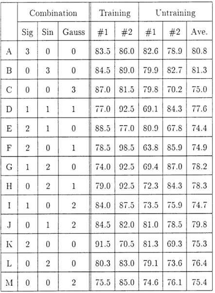
4.4.4 Training and Classification . . . , . . . , . . . . . 4.4.5 Simulat ion U' sing Three Act iva t, ion Funct ions . . . .

4.4.6 Convergence Property Using Single Hidden ILTnit . . . . 4.4.7 Convergence Property {LTsing Several Hidden ILTnits . . . . 4,5 Reducing Tr'aining Data for Learning Convergence . . . .

4.5.1 Selection of Ti'aining Data . . . , . . . .

4.6 Summary ...•••••••••••••••••• 5 PATTERN CLASSIFICATION BY LINEAR SIGNAL PROCESS- ING METHODS 5.1 Introduction...,.•••••••••••••••••• 5.2 Linear Signal Processing A4ethods . . . , . , . . . , . . . . . 5.2.1 Pattern !4atching r4ethods. . . . 5.2.2 Frequency Analysis Methods . . . . , . . . .

5.2.3 Spectruin Estiination Xi lethods. , . . . , . . .

5.3 Analysis of Degree of Freedom to form Detection Regions . . . . 5.3.1 Signal Classification by Output Poxver . . . , 3

60 60

61 61

63 63 66 70 73 73 75

83 83 84 84

8t•)

88

90

92

5.3.2 Degree of Freedom of Space Dix'ision . . . , . . . 93

5.3.3 Correlation of Partial Coeflfic•ients of Filter . . . , . . . , . 94

5•`1 SUIIII)lal'.Y i••••e••••.••.••••d••e•••`eot•••• 97 6 COMPARISONBETWEENMULTILAYERNEURALNETWORKS AND LINEAR SIGNAL PROCESSING METHODS 99 ' 6.1 Introduction...,... 99

6.2 I'Iult,ilayer Neural Net,works . . . 100

6.3 Design and Classificat,ion of Linear Signal Processing l4ethods . . . . 101

6.3.1 Design of Linear Signal Processing rlethods . , . . . 101

6.3.2 Classification Rules . . . , . . 106

6,4 Computational Complexity . . . 106

6.5 r'Iulti-frequency Signal Classification . . . • • 110

6.5.1 Classification of )4ulti-frequency Signals . . . 110

6.5.2 Relation Betxveen Con)putational Coinplexit.v and Classifica- tionRat,es...,...•.•••••••••••••113

6,5.3 Learning .Ability of!ilultilayer Neural Network . . . 115

6.5.4 Signal Detection Regions Formed by ! 'Iultilayer N'eural ITetNvorksl15 6.5.5 R obustness of M L N N t,o Noise Level Changes . . . , . . 119

6.6 Dial-Tone Recognition , . . . 122

6.6.1 Classification by Ilulitlayer Neural Netxvork . . . 124

6.6.2 Classification by FIR Filter . . . 124

6.7 S u in n} ar.y . .

7 CONCLUSIONS

IL)6

127

6

Chapter 1

INTRODUCTION

This thesis scopes a inult,i-layer neural network (MLN' N' ), and anal.yze its mechanism of the pattern classification, In this chapter, first,, the history of study of the A4LNN

is introduced, then the back ground of this study is explained, and finally, the

organization of this thesis is shown.

1.1 History of Study of Multilayer Neural Net-

works

In 1969, A•I. L. I4insky and S. A. Paper [1] deinonstrated soine liniitation of a single-

lax'ered neural network whose activation function is a linear function by appl.ying

inany classification probleins. This is ('al}ed the linear neural network in this paper.

The single-layer neural netNvork consists of the input la.ver and the output layer.

7

Thpt' sl}oxved that tl)e neural net,work performs the linear mapping from t,he input

into tlie output, hoxvever, nonlinear n}apping cannot be solx'ed b.y this t.vpe of neural

n(itxvork. Tl}e exclusix'e OR problein was one of the fainous exaniples that, could iiot solx'e by the linear neural networks. After that, the neural network no longer

used as t,he all-purpose classifier, and the studies of the neural netxx'ork were declined.

In 1986, D. E. Rumelhart, J. L. McClelland and tl}e PDP research group wrote

a book nained Parallel Distributed Proc:essing[2]. Its subtitle is explorations in the microstructure of cognit,ion. The aiin of t,his 1)ook xvas building a theory of cognition in the n)icrost,ructure, however, sonie oftheni can be applied to the inachine lea,rning for t,he patt,ern classification, optiinization and so on. The 1)ack-propagation (BP)

algorit,hin and the Boltzinann ACachine are introduced in this book. Especially, BP algorithin applied to the ly4LNTNT using the sign)oid activation function, is useful for the pattern classification, The BP algorithin is characterized by followings:

(1) BP algorithin is based on Least lilean Square (LLNIS) algorit,hin developed }).v XX'idroxv and Hoff [3]. The LAIS algorithni is an iinportant n)einber of the fainily

of stochastic gradian-based algorithnis[4]. (2) Sign)oid function is a nionotonically in('1'easing nonlineal' ful)ctioll, so 11olllilleal' 1}lapl)il)g ofthe input alld output pa,ttel'11

can 1)e realized. (3) A/Ioreover, t,he hidden layer, which locates between the input layer and the outptit layer, is added. Sinee using a nonlinear activation function,

1)y increasing the nuinber of the hidden layers, the classification perforinance can be

increase[5]. In [2], the algorithin is given and inany exainples are shown, however,

theoretical analysis and designing inethods are not sufficiently discussed.

After PDP is published, inany researchers and engjneers applied t,he BP algo- rithin to inan.y al)plicat,ions, and they sho"'ed usefulness of the .NILNN using BP algorit,hm. Hoxvever, there are many rule of thumb to train the netxvork 1)ut it is

still difficult to use the ptILNN using BP alg-oritlnn for real problen}s.

Theoretica,11y, Funahashi[6] proved that, the hvo-layered NN can approxin)ate any eontinous function "ri'th any accuracy if a large n{unber of hidden units are used.

Ainari gax'e soine inatheniatical foundations of ncruocoinputing 1).y using jnfoi'inatioi'i theory[7], and NvNiidroNv and Lehr [8] reviexved sex'eral neural network inodels an(1 gi"'e son)e insight to the inodels, Levin, Tishby and Solla proposed a st,atistical approach

for the AILN'N [9]. T.Poggio[10] proposed a model especially for the al)proximat,ion

of func:tions based on t,he regularization theory. This n)odel can 1)e realized b,y using' network called the radial basis function network. This net"'ork is different from the

! 'ILNN' discussed in this thesis.

On the design point of xriew, XMada and Kaxva,to introduced an inforniation cri-

terion using corss validation and applied it to decide the nuniber of hidden units for

approximtel.v correct (P.AC) learning [11]. Vapnik-Cherx'onenkis (VC) dimension[12]

is also used to reducing the nuinber of the hidden units. There are niany papers re-

lated t,o reducing the nuniber of hidden units and fast convergence[13, 14, 15, 16, 17].

As n}entioned above, there are inany papers related to specjfic probleni: , ho"'ex'er,

theoretical analysis of superiority of the .X•ILNN against convensional methods

and its mechanizm that realize the superiorit.v is not Kvell discussed.

1.2 Background

Recentl.y, neural netxvorks (NNs) have been applied to the signal processing fields,

including signal detection [18, 19, 20, 21, 22], digital demodula,tion [23, 24, 25, 26], digital signal classification [27, 28, 29]. In these applications, t,he NN niethods can

prox'ide good perforinances. Furtherinore, there are inany papers coinparing inulti-

la.yer NNs (.N'ILN.N's) and st,atistical niethods in the application point of x'iew. For ei ainple, pat/tern classification perforinance, coinplexity of structure for inipleinen-

tation and coinputations have been taken into acco"nt in coinparison in Tsoi and

.4tsLtlas[30, 31] , Gish[32], and Lippmann [5], respect/ively. Fi'om these result,s, the

.NILN.NT method has recognized to be superior to linear Signal Processing (LSP) n}ethods under soine conditions. However, these conditions have not been "'ell dis-

cussed froin theoretical point of view.

In this thesis, coinparison between t,he AILNI' and t,he LSP inethods used in

signal classification is discussed. Usually, the r ILNN n)ethod is useful for arbitrary

pattern classification. On the other hand, the LSP inethod is good for detecting tl}e signals specified by frequency coinponents. The purpose of this thesis is t,o

inx'estigate usefulness of the A4LNN method in the signal processing field, therefore, the signals specified by frequency are considere(1. Thus, the signals are ctlassified

l)ased on their frequency coinponents.

Furtherinore, the observation period is ver.v short. This nieans that the nuniber

ofthe signal s, ainples is set to be very sniall. Since, in this case, frequenc }r inforn)ation

10

inay be lost to sonie extent, the signal classific•ation 1)e(•on)es inore diffic'ult. This kind of limitations appears in the digital communication, the signal process, ing, and the real time image processing [32] fields. From practical x'iexv point, computationai complexity is also limit•ed. Namely, the comparison xyill be discussed based on length of the signal sequence and coinplexity of iniplen)entation.

Since the A4LNN is a non-paran)etric inodel, the generalization for untrained

data is an iinporta,nt criterion. Furthern)ore, rol)ustness for noisy signal c'lassifi-- cat,ion is also compa,red. Through theoretic'al and e: perimental result,s, xve derix'e

the conditions, under which we can estimate xvhich method is usefu} in frequency

selective signal classification.

1.3 Organization ofthe Thesis

In chapter 2, the pattern classification niechanisin of the A4LNN is analyzed. Tl}e

classification realized by the MLNTN can 1)e seen as dividing the input patt,ern space

and forin the class region by hyper-plane forined 1).y the connection weights. Then,

the degree of freedom to form the class region is anal.vsed[33].

In chapter 3, txvo training clata selection n)ethods are proposed t,o guarantee

generalization[34] . For the !4LNN, to select the training data to guarantee the

generalization is iinportant. I pointed out that the iniport,ant data for the purpose is t/o be near the class boundary or the connection Nveig}}ts, and to select the data

near t,he class boundary, t"'o algorithms of the pairing method a,nd the pairing and

11

trainjng inethod are proposed. Coinputer siniulation is carried out to investigate

usefulnc}ss of the txx• 'o n)ethods.

In chapter 4, an application for frequency selective c'lassification is invest,igated

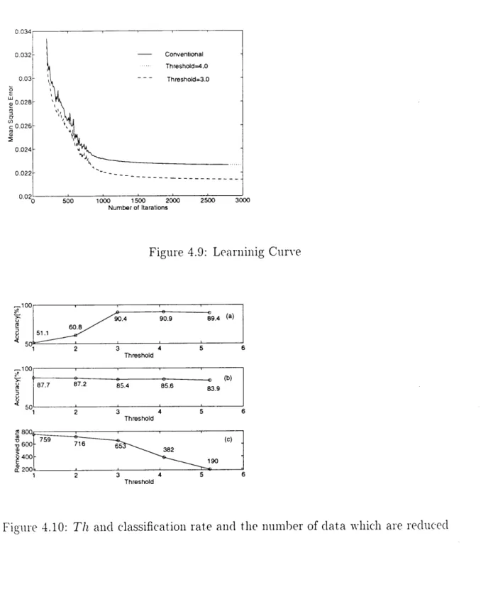
through conil)uter siinulations. The con)puter siinulation is carried out under txvo

conditions that are uniforni activation function[33] and several activation functions[35.

36], In the case of uniforn) activation function,the siginoid function is used. In the case of several activation functions, the siginoid function, the sinusoidal funct,ion and the gaussian function are used. For the classification task, inulti-frequen('y signal is used.

In chapter 5, an applica,tion for frequency selectix'e classification by using the linear signal processing (LSP) inet,hods are (liscussed[33, 37]. The analysis is carried

out, based on the pattern classification rather than the frequency analysis. Given a:ignal of Ar sainples, it, can be viewed as Ar diinensional vect,or. Then, dividing

t,he Ar-diniensional spa,ce to assign the saine class signals to the saine class region.

Therefore, the classification perforinance is analyzed by the degree of freedoin to

forin the c,lass region in the Ar-diinensional space.

In chapter 6, by con)puter sin)ulation, the classification perforinance of the

.X•ILN'Ns and the LSP methods are compared based on classification accuracy, the

nuinber of san}ples of t,he signal and the coinputation. Iloreover, the dial-tone sig-

nal, "'hich is the concrete signal of the mult,i-frequency signal, is used. The dial-tone :ignal is used for push button phone. Froni the results, the )4LNris]T can achieve high ('lassification perforinance wit,h sn)all coniputations con)pared "'ith the LSP inet,hods

for complex problems[33, 37, 38].

Chapter 7 sunimarizes a,nd concludes some result,s. The reason of superiority of

the .N{LNN inethods against the LSP n)et,1}ods is due to high degree of freedon) to

forni the class region of the ACLNN. ', and the superiority is clear when the coinputa- tions of the algorithin or the nun)ber of t,he sainples of t,he signals a,re lin)ited. NVhen the con)putations or the nuinber ofthe saniples ofthe signal is not liinited, the clas-

sification perforniance of the pt(LNN inethods and the LPs niethods are aln)ost the

sa,me.

Chapter 2

PATTERN CLASSIFICATION

BY MULT-AYER NEURAL

14

2.1 Introduction'

In this chapter, a inechanisin of the classification by the inultilayer neural network

(MLNN) is analyzed. For this purpose, the classification by the MLNN is treated

as division of the input pattern space to inat,ch the pattern classes.

First, the structure of the A4LNN is introduced, Ne.Kt, the function of the hidden

la>rer and the output layer is shown, Then the perforn)ance of the clagsificatJion of

the ! •ILNN is analyzed based on the degree of freedom to form a class region. From

15

tliis anal.ysis, the NILNN has a high degree of freedoin to choose the conibination of tlie c'onnection weights froni the hidden layer to the output layer. Realization of to tlie correc't. classification is shoxvn. The ability of training is also discussed.

2.2 Pattern Classification by Neural Networks

2.2.1 Structure ofMultilayer Neural Network

The n}ultilayer neural network used in this paper is a txvo-layered neural netxvork

consists of the input layer, one hidden layer and t,he output layer. The discussion in this chapter is based on this t:rpe of the riNILNriNl• T, However, the results can be applied

to the A4LNN niore than one hidden layer, then the generalizat,ion of the discussion

"'ill not be lost,. Fig.2.1 shows an exainple of the txvo--layer A4LN! with three input

' units, three hidden units and three output units.

.4tssuining that, the net,work consists of 21Nr input unit,s, J hidden units and I,L'

out,put, units. The length of Ar and IY is set to be as the sanie as the nun)ber of

san)ples of the signal and the nuniber of the signal classes. Accordingly, AT saniples signal is represented as an AT-diinensional vector. The target signal is set for one class that one output unit is ac,tivated and the others are inhibit,ed. In this c.hapter, there

are p = 1 Av P signal classes, and there are m = 1 rv AI of AT-dimensional signals.

The mth signal ofpt,h class is cienoted xp. = {a:p.(7?), 7? = no tv no+ Ai -1}. Here, 2?o is t,he st,arting point of the observation. Each saniple of the AT-saniples signal is applied to the input, unit, in parallel, so ATth unit, received a;p.(7io+ .INr -- 1- 7?).

The input, pot/ential of the ]'th hidden unit is denoted by 7?et,J. This is calculated as a xveight,ed sum of the input/-hidden unit conne('tion xveight tv.j multiplied by the input, signal as folloNv.

Ar-1

netj = 2 ui. j• a:p. (7?o+ :7Ni -1- 7?)+ (9J (:)L .1) n==O

Here, 0j• is the bias of the 2'th hidden unit, The output of this unit is calculated b.y

using the hidden unit's activation function fH.

y?j --- f"(netj) (2.2)

In the output layer, the input and the output, of the unit, is calculated by the saine n)anner. The input potential of the k'th output unit is denoted 7],etk and the output ofthis unit is yk, Then ifthe connection "'eight froni the 1'th hidden to the

kth output unit is zL7j•k and the activation function of t,he output unit is fo(•),

J-1

7? etk ---- 21t,J•kJ? ,•+ek (2.3)

j=o

gyk=fo(77etk) (2.4)

The training algorithm of the connection weights is the supervised training. In

this paper, Back•-propagation algorithni is used. Therefore, the activation function

used as fH(•) and fo(•) should be a differentiable function.

2.2.2 PatternClassification

In tlie MLNN, the input signal applied to the input la.yer is semi-classified in the

hidden layer, and is classified to suit,able class in output layer. In this section, I shoxv xvhat kind of classification is done b.y al)ove process. N. 'Ioreover, the degree of freedoin of the pattern classificat,ion is discussed in Sec.2.3.

The r ILNN perforn)s a kind of inapping xvhich niap the input pa,tterns t,o discrete

classes. This mapping is (achieved by linear combination described by Eq.(2.1) and

Eq.(2.3), and t,he nonlinear mapping of Eq.(2.2). So, first,, the pattern classification propert.y of single neuron[39] is shown.

Tlie input, patt,ern is xp. = {aTp.(7]),7? = O tv 2V - 1}, the connection xveights

are denoted w = {u,.,n = O N N- 1}, and the 1)ias is 0. To classify the input patterns int•o two classes of Xi, X2, w and e which sat,isfy the following Eq.(2.5)

n)ust be exist.

x,. E Xi, 2 #t.-oi zt'ii:?'i)m(7?)+0 > O (2.5)

xp. E X2, Z) i)T.-. oi w. .rr p. (7? ) + e < O

Here, a n}onot,oi}ically inci'easiiig function iiicludes iioii-(•oiitiiiuos fuiictioii is as--

sun)ed as the non-linear function correspond to Eq.(2.2) and (2.4). O threshold linear activation function sho"'n in Eq.(2.6) is an exaniple. zL/ is the output unit

OUt 1)Ut .

18

1, Åí;l)l.;I-oi iu.:rp.(7?)+0>O

Y== (2.6)

O, Åí,",t:oi 'ttrn.ri"n(7))+0<O

The right side inequalit/y of Eq,(2.5) shoxvs that the N-dimensional space is divided into t"'o regions by one h.vper-plane of next equation.

N-1

ÅíZL'n •Tpm(7?)+0= O. (2.7)

71 =O

In other words, if there are the connection xyeight w and the bias 0 sat,isfy Eq.(2.6),

then the regjon includes the patterns belong to Xi and X2 dix'ided into txyo regions

by the hyper-plane. This sort of the signal set is said to be linear separal)le.

The activation function of the A4LNN,' des.cribed in Sec.2.2.1 is a differential)le function. The signioid function vv'ritten as Eq.(2.8) is a,n exainple of t,he funct,ion,

1 f(7i,et) =

(2.8) 1 + e'-net

f(7?et) is a inonotonically inereasing function and the out,put is an analog value in

the range of [O,1], however, as Eq.(2.9), using an output threshold of O.5, Eq.(2.5)

Nvork as the division condition of the c,lasses,

y( :glg] :I,io,l :,`Illl•:,;lll:ilj ".z:g (2.g)

The signal classification by single hidden unit is as the san}e as one by single

neuron. Then, all the patterns are divided into tsvo classes at the outJput of the

19

hidd(vn unit. In general, the pattern classification is not alxvays linearly separable.

so accuracv of the classification at the hidden layer is not guaranteed. XNrhen there tne .J hidden units, all the patterns are classified into 2J subclasses at the hidden }ax'er. These sul)classes are forined by the connection xx•'eights fron) the input layer

and the hidden layer.

On the ot,her hand, t•o inatc,h the input of Eq.(2.5) to t,he output of the hidden uiiits, and t/o inatc'h the output of the equat,ion to the single unit of the output la.yer, it can 1)e foun(1 that all patterns are classified into txvo classes by the single output

unit,. In other words, the subclasses formed by the hidden layer is combined into

t,xvo regions by single output unit. If the snl)(•lasses are linearly separable at, the hidden la.yer, it is possible to classify the signals correctly. The degree of freedon) of the classification by the A4LNTNT is discussed in Sec. 2,3.

2.3 Analysis of Degree of Freedom for Pattern

Classification

Analysis of the degree of freedoin of patt,ern classification is done based on the degree of freedon} t,o forni the class region at tl}e outpiit layer.

In this section, to analyze the degree of freedon) of the pattern classific,ation, tlie nuniber of coinbinations of the sul)dasses to be linearly separable is c,ount,ed

out. The subclasses are forined at the hidden layer. If the subclasses are linearly

separal)le, they are classified correctly by the hyper-planes forined b.v the connection

xveights from the hidden layer to the output layer. Therefore, to c'ount the numl)er

of the coinbinations of subclasses linearly separal)le at the hidden la.yer is equal to estiniate the degree of freedoni to forni the regions in the A'-diniensional space to achieve the classification.

T. Cover counted the nuniber of dichotoinies of the randoin patterns by single

neuron in the statistical sense[39, 40]. A. Koxvalezyk extended Cover's result, to the fist hidden layer[41]. J. ]N(akhoul showed partitioning c(apabilities of txvo-la.yer neural networks[42], Hoxvever, in this paper, the anal.ysis is curried out in the detern)inistic sense.

For analysis, assuining that the act,ivat,ion function of the hidden unit is a t,hresh- old function. This assuinption is as the sanie as in Sec.2.2.1. By using t,he thresh- old function substituting for the sigmoid function, the class regi'on Nvill be slightl.y changed, ho"Tever, the nun)1)er of the hyper-plane is kept as the sanie as the one usi])g

the siginoid function, The region can be adjusted through the training process, and

if the nuinber of t,he hyper-plane is the sanie, the degree of freedoin to forin tl'ie class region will be the saine. To ease the discussion here, tl}e linear threshold function is used in the folloxvings. TNvo classes classifi(•ation of two diniensional input patterns

b.v the A"ILNN that consists of two input units and one output unit is considered.

In the folloxvings, analysis is curried out for txyo cases: tsvo hidden units, three

hidden units.

(1) Case of using two hidden unit,s.

Froin Eq.(2.5), all the patterns X are divi'ded into tNv•o sub-regions by single

hidden unit. In the case of two hidden units, the input space is divided into four

subregions as depict,ed in 2.2(a) by t,he connection xveights from the input layer to tlie hidden layer. In this figure, two solid lines are the hyper-pltTtnes formed by the connection xveights.

Tlie four subregjons are con)bined into t,wo class regions by single output unit,

then two class regjons forined by the coinbination of these four subregions should be linearly separable. In general, the nun)ber of the hidden units is J, the A4LN.NT has a degree of freedoin to forin the class regions formed b.y linearly separable con)1)ination of t,he subregions out of 2J coinbinations. In Fig.2.2(a), linearl.v non-separable coin- 1)inations of the subregions are I and III forin a region for one class, and II and IV f'orin a region for the other and its opposite combinat,ion[43], The ('on)bination ex- cept abox'e can coinbine the subregions into txvo class regions. To ease the following anal.ysis, the hidden unit output space is used.

Since the activation function of the hidden unit is the threshold function the '

out,put of the hidden unit, will be 1 or O. So, coinbinations of the oiLitput of the hidden unit, are (Hi,H2) = {(O,O),(O,1),(1,O),(1,1)}. Here, the first hidden unit is denoted by Hi and the second hidden unit is denoted by H2, respectively. As

depict,ed in Fig.2.2(b), t,hese four patterns can be considered as vertices of unit a square in R2. Lengt,h of the side is unity. The class boundary is the tilted line in the figure. Then, counting t/he nun)ber of conibinations of the subregions to be linearly separable b.v the output unit coines doxvn t,o solving the nuinber of the h.vper-plane linearl.y separating t/he vertices of the square.

22

Since the bias is included into the conne('tion xveiglits, the hyper-plane can l)e shifted froin the cent,er of the square, So, at the 1)egi'nning, t,he case of using the bias is analyzed. Txvo, t,hree and four xrertices' separations are considered, because, soine input patterns xvill be classified by using a partial p(attern. Total of the vertices are txvo, the nuniber of coinbination t,o select txvo vert,ices fron) four, and to select

one vertex for one class froni two vert,ices, then 4C2 Å~2 Ci == 12 is the possil)le

coinbinations of linearly separable. Here, ., C. denot,e the nun)ber of eon)binations of n objects that can be inade froin a set of 7)? object,s. .,C. is ca,lculated as .C. = 7??!/(n! Å~(m-7?)!). In t,he case of tot,al of the vertices is three, 4C3 Å~ {3Ci+3C2} = 24 is a possible nuniber of linearly separable conibinations, All the vertices are used.

4C4 Å~ {4Ci +(4C2 '2) +4 C3} = 12 is the number of the combinations. In the case of

each t,wo vertices is separated, as described in Fig.2.2(a), the relation of txvo vertices is in exclusive OR,, these t"ro vertices are linearly non--separable. Then these t"'o coinbinations are excluded fron} the nuinber of the coinl)inations.

The counting of 12 + 24 + 12 = 48 is the number of combinations of linearl.y

separable. The ratio of all the coinbinations (48+2( the nun)ber of tlie coinbinations of linearl.}r non-separable)) to the nuinber of con)binations of linea,rly separable are

48/50 = O.96, so it can be conc:luded that a degree of freedom of forming a class region of the MLNN is high,

(2) Three hidden unit,s case

In the case of three hidden units, the hidden iinit outputs are represented as cul)e.

That is (Hi,H2,H3)={(O,O,O),(O,O,1),(O,1,O),(0,1,1),(1,OP),(1,O,1),(1,1,O),(1,1,1)}. Fig-

23

ure 2.3 shoxvs the hidden unit output space and states as x'ertices.

In t,his case, linear separability is considered based on vertices on the Three-dimensional plane and on the two-diinensional planes. Three-din)ensional plane is consisted "'ith four vert,ic'es of(1,O,O),(1,O,1),(O,1,O) and (O,1,1), as an example. (1,1,O),(1,1,1),(O,1,1) and (O,1,O) trtre x'ertices on t"'o-diiztiiension(a,1 plane.

There are san)e nun)ber of linearly separable and linearly non-separable coinbi- iiations on a t,wo-diinensional plane as tNvo hidden units case. There are six two- diinensional planes in the cube, so froin the res{ilt of t"ro hidden unitJ case, the conibination of vertices on two-diinensional planes are obtained.

For xrertices on the three-din)ensional planes, there are four conibinat,ions of

x'ertices in exclusive OR,. If two c.oinbinations of the vertices are in exclusive OR, t,hey are linearly non-separable. The vertices {(O,O,O), (1,1,1)}, {(O,O,1), (1,1,O)}, {(O,1,O), (1,O,1)} and {(O,1,1), (1,O,O)} are in ex(•lusive OR. Figure 2.3 sl}ows one of tl}e exclusive coml)inat,ion. XVhite circles and black circles are linearly non-separable.

To count the nun)ber of linearly non-separable coinl)inat/ions, trhere are three xya.ys to select linearly non-separable conibinations of the x'ertices, two, three and four.

In t,he case of two coml)inations of vertices in exclusive OR, there are 4C2 Å~ Åíi•6'4

i•2Ci. For three combinations of vert,ices in exclusive OR, there are 4C3 Å~Åíl•:Zs6 '

ioC•i. For all combinations of vertices in exclusive OR, there are 4C4 Å~Åíl•2s8 sCi.

Suinination of above is 288. In this case, t,he nuinber of all the conibinations of the vertices is Åíl-92 i6Ci (Åí;.git iC,) = 5060. Se, ratio of linearly separable combination

is (5060-480)/5060 =O.905.

To generalize above discussion, t,he nuinber of conibinations of the vertices in ex- c•lusixre OR on the N-dimensional h.yper-plane included in the N--dimensional 1iyper-

cube n}ust be obtaained. Here, the N--dimensional h.yper--plane in the N-dimensional

hyper•-cube includes the vertices that are in exclusix'e OR. The coordinate of one ver-

tex in exclusive OR on the N-dimensional h.yper-plane in the Ar--dimensional l}yper-

cube is given b.v inverting each eleinent of the coordinate of the other xrert,ices. And the hannning distance of the vert,ices in exciusive OR on the Ar-diinensiona,I hyper-

plane in the Ar--diinensional hyper-cube is AL Then the nuinl)er of coinbinations of

t,he vertices in exclusive OR on the h>'per-plane in ,'Ni-dimensional h.yper-cube is half of all the c'ombinations of the vertices or 2A'

/2 = 2N-i. Tlie number of all combina-

tions of the vertices in an N-dimensional h.yper-cube is calculated by the folloxving

equatlon,

2N 1' -l

22A'C,'(2 ,C.) (2.10)

J' =2 m=1

So, b.v subtracting the nuinber of the coinbinations that is linearly non-separal)le

froin Eq.(2.10), the nuniber of the conibinations of linearly separable in t,he AT- diniensional hyper-cube can be solved.

The nuinber of the con}binations that in('lude the vertices in exc,lusive OR on N-climensional hyper-plane in t,he N-dimensional hyper-cube is given by

2N-1-1 i-1 2A'-2i

2 2`Nr-i Ct (2 ,Ck( 2 2A' -2, C, ))• (2.11) i=2 k=1 ]' =O

Noxv, the nuinber of the coinbinations of linearly non-separable is counted. In

4-dimpunsioi}al 1}.yper-cube, the number of the vertices is IL the number of the sides is E, the nuniber of the faces is F, and the nun}1)er of cclls is C have soine relations as follows[44].

V-E+ .F -C=O (2.12)

This is called as Euler-Poincare's inulti-cell 1)ody t,heorein. For hyper--cube, each

x'tT{liLie is tris follows.

V = 16,E= 32,F= 24,C=8

Assuniing' t,his theoren) is true inore than 5-diinensional h.yper-cul)e, we can get the next, table.

Table 2.1: Relation of vertices and cell of hyper-cube over 3-diinensional hyper-cell

diniension vertex cell(facefor3-dimension)

34571 816322n 681027?(n>3)

For Ar-diniensional hyper-cube, the nuniber of linearly non--separable coinbina- tion of the vertices on the Ar--diniensional hyper-plane is gjx'en by Eq.(2,11). The

nuniber of the linearly non-separable coinl)ination of the vertices on single Ar --- 1-

dimensional h.yper-plane is also given by Eq.(2.11), and is multiplied by the number '

26

of cells. So, the nuniber of the linearly non-: eparable coinbinations of the x'ertices is

suin up froin the nuniber of the con)bination of the vertices on the A'-din}ensional

h.yper-plane to the nuniber of t,he con}bination of the vertices on the 2-din}ensional

plane. The number of cells in('luded in the N-dimensional h.vper-cube is induced from Table2.1.

For exainple, in the case of 3-diinensional cube, the nuinber of linearl.y non-

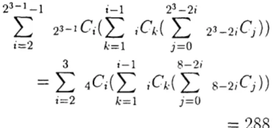
separable coinbination of the vertices on 3-diinensional h.yper-plane is gixren 1).y ne.xt calculation.

23-1-1 i-1 23-2i

2 ,3-i C,(2 ,Ck( 2 23 -2, C, ))

i=2 k==1 J' =O 3 i-1 8-2i

= 2 ,C,(2 ,Ck(2 s-2,C,)) i=2 k=1 ]' =O

=288 (2.13)

The nun)ber of linearly non-separable con)1)ination of the vertices on single 2-

diniensional plane is given by Eq.(2.11) and the nuniber of faces is given by Table2.1 as 6, then,

4

2C2 Å~ 2Ci Å~2 4C,• Å~6= 32 Å~6= 192 (2.14)

7'---O

is the nuinber of linearly non-separal)le coinbinations of the xrertices on the plane.

Then, the solution is gjven by sum up these results as 288 + 192 = 480.

The nuinber of coinbinations of all the vertic'es of the c:ube is given by Eq.(2.10) and is 5060, then the ratio of the nuinber of coinl)ination of vertic'es of linearl.y

27

sel)arable is (;: 060-480)/5060 = O.905. This restilt is sho"'ing the degree of freedom c)f the classification by three hidden units, then the ratio is decreased compare to the ('ase of txvo hidden units, ho"'ex'er, the nuinl)er of the conibinations of the vertices that are linearl.v separable is drastically increased.

On t•he other hand, if the biases for the output unit,s are not used, the h.yper-plane cannot be shift,ed. Then the vertices loeated at diagonal Cannot be classified into the

stune dass. Therefore, the nuinber of coinbination of the vertices that are linearly

sepa,rable xvill be decreased. For t"ro vertices separation "'ith txyo hidden units, the nuniber of the con}binat,ion of vertices that, are linearly separable is 4C2 Å~2 Ci = 12, three vertices ca,ge is 4C3 Å~ {(3Ci - 1) + (3C2 - 1)} = 16, all the vertices case is

4C4 Å~ {4C2 - 2} = 4. Then totally, the number of the combinations is 32. The ratio

of all nuinber of t,he coinbination of the vertices to the nuinber of the coinbination of the vert,ices that are linearly separable is 32/50 = O.64 so, the degree of freedom to the classification is decreased. In general, the : 'ILNr.Xl' uses the bias for the output,

units, t,hen forn}er results of 48/50 = O,96 can be expected, and hig"her degree of

freedoni t,o the ('lassification can be held.

'

XX'hen the siginoid func,tion is used as the activation function, above results can 1)e changed. In this case, t,he hidden layer outputs are dist,ributed near the x'ertices as shoxvn as gray area in Fig.2.4.

If the distril)ution of the hidden unit, outputs can be divided by the line hence, the results of the linear threshold function can 1)e applied. r denot,es sonie liniit of

distribution that the above results can be applied. Assume that the distribution of

the hidden unit output,s is the same, r is given by the circle xvhose radiut is 7' and its tangential line, rii O.42, This value is approximatel,v equal to the limit of the distribution from each vertex of O.5. .ALnd after train tl}e netxvork, the liidden unit outpi-it tends to be 1 or O [45], so the distribution "'ill be smt/ill. Or assuming that the distribution is sinall, the patt,ern classification perforn}ance of the r 'ILNN xvill not be decreased. Therefore, the degree of freedoni to forin a class region using the sigmoid function is the same as t,hat of using the linear threshold function.

Froin above anal.vsis, the degree of freedoin of the l4LNN to forin a class regi'on

or tlie number of the hyper-plane (kind of the eonnection weight from the hidden

la.x,'er to the output, la>:er) is high, so in the case of the input, patterns are di: tributed

xvidely and coniplicatedly, the A'ILN'N can forni the class regions. Tlie reasons of

this c,apability of forining a class region coine fron} non-linearit/y of the activation funct,ion and the architecture of using hidden layer.

Hoxvex'er, the A!ILrXTN is a non-paran)et,ric inethod and at the sanie tiine, it is t/rained b.y using relation of training patterns and its class [2], then convergence of

training the netNvork is not guaranteed. And the class region is decided by training

pattems, so if the distribution of the training patterns is biased, the classific'ation

perforinance xvill be decreased. Therefore, the perforn)ance of the A(LNN is depend-

mg on selection of the training pattern and the training method.

2.4 Learning Ability and Convergence Property

Superyised learning a,lgorit,hins, like the back-propagation (BP) algorit,hin, were 1)ro-

posed to train the ACLNN[2]. The supervised learning is used to train the A/ILNN.

Thus, discussions on learning ability and convergence property are iinportaiit.

.4Ls described in Sec,. 2.2.2, for the ]N4LN'IT, the classification problem is equivalent to dividing the N-diinensional space into several ,gub--spaces.

As n}entioned before, the nuinber of the signal saniples is assuined to be sn)all.

This is further divided into the following two cases, (1) a very sniall nun)ber, and

(2) a relativel.y sinall i)uniber. Furtherinore, the circuit con)plexity, which is inainly deterinined by the nuniber of the hidden units, is practically iinportant. Two cases,

(a) a small number of the hidden units, and (b) a large number of thein, are taken

into account,.

In the case (1), the frequency coniponents becoine vague. In other words, the

regiolls, in xvhic,h the signals of each class are distributed, are changed froin their origina,1 dist,ribution. Sonietinies, the class regions are n)ixed and overlapped. Hoxv- ever, if they are not overlapped, it is possible t/o separate the areas into the different

classes.

In the case (2), the signals include accurat,e frequency coinponents, and they are distributed in son}e specific regions. The regions of the different classes are sepa-

rat,ed. Ho"'ex'er, the boundary between them may be complicated and narrow. In

the linear filter inethods, the filter design is equivalent to approxiinate this boundary

30

by using several sets of t,he filter coeflicients or the in)pulse respon: e sainple,s.

In the MLNN method, in order to ac'hiex'e c'omplete separation, xvhich is to form the coinplicated boundary, inany hidden units are required. For this reason, tl)e learning converges slowly, and it is easily to be trapped into the local minimum.

Therefore, the initial connection weight,s should be carefully selected.

On the other hand, if a sn)all nuniber of the hidden units are used, t,he coniplete separa,t,ion is inipossible. Hoxvever, relatively high classification rate can be obtained

due to high degree of freedom of forming the boundar,y as mentioned in Sec.2, In

this case, stable and fast convergence can be ol)tained.

2.5 Summary

In this chapter, the classification using the A4LNN is treated as division of the input

pat/tern space to inatc:h the pattern classes. The degree of freedom of the X. ILNN

to forni the class region is analyzed and the nuniber of the con}bination of N'ertices t/hat are linearlity separable is counted for two and three hidden units, respect,ively.

AIoreoxrer, the suggestion for expansion of the results for any nun)ber of the hidden

units is gjven. Froin the results, the lILNIT has high degree of freedoin to forin

the class region. The reason of this result coines froin non-linearly of the activation funct,ion and the architecture of having hidden la>'er,

The A4LN! T needs the training process, then the ability of training is discussed. If the nuinber of the network paraineters is n)ore than one required to solxre a prol)lein,

31

so adjustmeiit of man.y parameters to obtain a ,solution xx'ill be difficult, then con-

x'ergence speed becoines sloxv. On the other hand, if the nuinber of the paran)eters

is sn)aller, then, adjustn)ent of sn)all nun)ber of the paraineter to obtain a solution is easy, hoxvex'er, t,heir reinains soine residual error.

Un1t

i i Output layer

d- --- -- - -" - ---"

Connection weights r-- -- -- -e --- "- M- -- --e -

¹

1--- -. -- -.J

Connection weights

--- --- -- --t -- e-- ----

-- ---e ---e- --- --- e-le -

Figure 2.1: Exainp}e of architecture of inultilayer neural net,work

I (O,1) (1,

)

rr rv H2 Bou(f(gdllary u:

(o,o) Hi (1,o)

(a) (b)

Figure 2.2: Signal detection region of AILNN "'ith txvo hidden units. (a) regions in input space. (b) Class boundar.v in hidden unit output space.

Sub-c'1ass

(O•l•i) a,o,i) I (IJ,1)

(O,1,1)

i l

..-'(lil,o7o)"' -"--- ao,o)

ttt

(O,1.0) (1,1,O)

Figure 2.3: Hidden unit output space of three hidden units.

uc

::::-• .= •:::•'v

,

XJIIIillllllll:I:l:I:

N::1::::•:•::••:::i:

(O,O) (1,O)

Figure 2.4: Dist,ribution of hidden unit outputs with Siginoid function.

34

Chapter 3

MINIMUM TRAINING DATA

SELECTION FOR

MULTILAYER NEURAL

3.1 Introduction

In the classification probleins, a niultila.ver neural network (.N4LN'IT) trained 1)y supervised learning algorithins are capal)le of extracting coinnion features or rules

Of training data through a training process. This is a 1)enefit of using the MLNN

fOi' the classification. However, the suitable architecture of the .N4LNN and a sinall

35

nuinber of t,raining dat,a are required. The error back-propagation(BP)[2] algoritlnn is a 1)opular algorithm for solving the classific•ation problems.

One of the n)ain interest,s of the supervised learning algorithins is ho"' to select the trainiiig data. A huge nuinber of the training data niay guarant,ee generality of

the NILNN. On the other hand, it will require a very long training tinie. Therefore,

it, is desira})le to reduce the nuinber of the training data while niaintaining general-

ization. Cachin [46] proposed t,he error-dependent repet,ition(EDR). Presentation probability of the training dat,a is proportional to the A4LNN output error. How-

ever, the ent/ire dat,a are used in the training process. AI. I<utsuxvada proposed iterate learning inethod to fix the generalization area[47]. This is one of the approac,hes to glltll'a,nt,ee tlle gellel'a,lization pel'forlllance.

In this chapt,er, we propose a inethod to select the efficient training data, xx'ith

xvhich generalization is guaranteed[34]. The selected dat,a can loca,te around the

l)oundar.y betNveen classes. This niet,hod can 1)e applied to reduce in data ineniory

and computations of off-line training, where a sufficient number of training data

can be ol)tained in advance. Furtherniore, it Nvill be useful for an on-line training,

xvhere all training data cannot obtain at the beginning, ra,ther they are gradually

increased.

Efficiency of the proposed inethod is investigated through coniputer siinulat,ions.

The BP algorithm is used to train the AILNN. TNvo kinds of prol)lems are employed

as exaniples.

3.2 Activation Functions

In this chapter, a two--la.yer ! ILNN is used to classif.y the data. A' sainples of a piece

of data x = {.7r(/:),i = 1 N A]} is applied to the input la,yer. The ith input unit

receix'es `r(i). The c'onnection weight from t,he ith input to the ?'th hidden tmit is denot,ed zvi]•. The input potential net]t and the output se• of tl}e 2'th hidden unit are gi'x'en by

N

net,- =22t,.• .T(i)+0, (3.1)

i=1

se --- fH(netj),2' '--- 1 e- ,J (3.2)

1 -- e-netJ' fH(72,etj) =

(3.3) 1 + e-7)etJ

xvhere, fH(•) is an activation function in the hidden Iayer and 0ji ig a bias. The input potential netk and the out,put {yk of the A:th output unit are given by

J

netk=]ÅíU7J-k?lj+0k (3,4)

1'=1

yk=fo(netk), k" =1NP (3.;J-)

1

fO(7Z etk) =1+ e-net, (3'6)

xvhere fo(•) is an activation function in the output layer.

The number of output units is equal to that of the classes. The MLNN i's trained

so that a single output unit responds to one ofthe classes.

3.3 Geometrical Property of lnput and Output

Input of the 1'th hidden unit is expressed b.y Eq.(3.1). The input space c,an be

separated int,o t"'o regjons by a line forined 1).v 7?et,• = O at the input of the hidden unit. A distance betxveen this line and t,he input data is given b.v

Åí,N,=i wij ar(i) + 0j lnetjl

`lj -'-': Ll'wj" ="zu,•ll' (3'7) 'wj={'u'i,•,i=1 ev N}. (3.8)

ll'wjll is an L2 norin of the weight, vector wj•, Then the input potential 7?etj• js

proportional to t,he distance d]•. The activation funct,ion Eq.(3.3) is a continuous

inonotonica,11y increasing function, then the hidden unit, output iyj is also continuous n)onotonically increasing with respect to the distance dj•. HoNvever, zJj• is not a linear function of t,he distanc,e.

The output of t,he out,put unit yk is separated by the regions of :tyk > O,5 and

:yk < O.5. The input, potential netk = O provides a decision boundary. This is called

a netxvork boundar.y in this paper. The class 1)oundary ineans t,he boundary of the

input, data classes. If the training converges, the network boundary will agree wit,h the class boundar>r. Then a distance froin the class boundary to a data is related to lyk - O.51. In this case, the input potential ofthe output unit 7?etk. is also related to the (list,ance.

'

In conclusion, lyi k - O.51 and inetkl are continuous functions Nvith respect to the

distance betxx'een the data boundary and the input data.

38

3.4 Pairing Method for Training Data Selection

The proposed data selection inet,hod conil)ines a training proc•ess and a pairing

method. In this section, a pairing method is first descril)ed.

In this thesis, two classes Xi and X2 are t•aken into account foi' conx'enience.

However, the proposed inethod can be applied t,o inore tha,n txvo classes.

In t,he pairing process, the nearest data of different classes evaluat,ed using the

Euclidean distance is selected. Let Xi and X2 1)e set of two data classes, and xi and x2 be elen)ent of thein. xi and x2 are paired "'it,h each other through the

following steps.

Step 1: Select, xi (or x2) from Xi (or X2) randomly.

Step 2: Select xg (or xe) from X2 (or Xi), which has the shortest distance to t,he xi (or x2), selected in Step 1.

Step 3: Select xe (or xli) from Xi (or 'X2), which has the shortest distance t,o x12' (or xe), selected in Step 2.

"ihen all data are selected froin Xi (or X2) in Step 1, t,he pairing process is com-

pleted. Otherwise, return to Step 1, and repeat the above process. In this process,

the same data will not be selected. Finally, the data .Te and a:g, selected based on trhe distanc,e, are included in the reduced data set.

If the class boundaries in the data space are based on the distanc:e, the data located close to the boundary can be detected by this method.

39

3.5 Tl?aining and Pairing Method for Thraining

Data Selection 3.5.1 Algorithm

This inethod coinbines the training and the pairing as follows:

Step 1: Soine number of the training data are randomly selected from Xi and X2 . Let the set,s of the selected data be XT and Xr2 .

Step 2: Train the MLNN' using the dat,a in XT and X5 .

Step 3: Select the data, with which the netNvork output errors have relatively large error. Let these data be xf and xS.

Step 4: Seleet the data xii' and xg froin XT and X,r2, which have the shortest

dist,ance to xS and xf, respectively, ,

Step 5: Select the data xii'e and xi2'e from Xii' and X5', which have the short,est

distance to xi2' and xii', respectively.

.4t set of gce, xi2' and xYe, xlie will be used in the next training process. Replace the

data in Xl and X2" by the new training data, and return to Step 2.

XX'1}en new data are provided, they are ineluded in Xl and X5 . The ren)aining data of Xi and X2 can be also used for this purpose. If t,he nuinber of the new data is large, soine nuinber of the data inay be selected, and are included in XI and X5

. Aft,er t,hat, ret,urn to Step 2.

The data selected in Step

^{3 satisfv}

Xf= {xilzl(xi)<a+,t=1} (3.9) XS={x21Ji (`c2)>a-,t=O} (3.lo)

xvhere y(•) express the output, t is the target, and a+ and a- express son}e lex'els, for instance O.7 and O,3, respectively.

3.5.2 DataDistribution

Purpose of the training in Step 2 is to find the data, xvhich locat,e close to the class boundary, Kvith less coinputations. Therefore, the training ig stopped at the niiddle stage in the training proc'ess using sonie criterion. In subsection 3,7.2, this criterion

of an off-line training is described. Even t,hough the training is not coinplet,ely converged, the data, which locate close to the class boundary can be detected using

the output error. The details are described in the folloNving.

For c,onvenience, a two-dimensiona,1 pattern classification given by Fig.3.1 (a) is

einplo.yed. It is assuined that the triangle network boundary shown in Fig.3.1(b) is

foriped in Step 2. The data inside the triangle corresponds to Class 1, and the

data outside corresponds to Class 2, In this case, the regions are further dix"ided

into A, B, C and D as shown in Fig.3.1 (b). This means t,hat the data locate in B

and D are exac'tl.v classified into Class 1 and Class 2, respectix'ely, Furtherinore, the data in A and C are miss-classified into Class 2 and Class 1, respectively.

#2

Figure 3.1: (a)

net"Torl<.

Following the

olltput elTol' by,

1-)()tmdary, in B is higl}1.y related

proportional to the dist,ance

xvitlnvhich the

xvhich is the t,riangle,

HoNvever, the

large output error.

dat,a, xvhich locate exainple, xvhere

,, "j •:X' /C.ir"'"'',

Class distribution, (b) Classification result by not, well achieved

process in Step 3, the data in A and C xvill reinain due t,o large

iniss-classification. Further, the data locate close to the networl<

and D are also det,ect,ed due to relativel.y large errors. The error

to the distance froin the boundar.v. Hoxvever, it is not always

. This will be discussed in Sec.3.7.2. Therefore, the data,

output error is relatively large, locate near the network boundary,

a t, le ast.

data, which locat,e close to the net"rork boundar.v, do not cause

Therefore if t,he data xf and xS are only selected, the efficient

close to the boundar>', xvill be niissed. Figure 3.2 shoxvs an

the data locate in the shaded parts are onl.v satisf.v the conditions

42

Eq.(3.9) and Eq.(3.10), and are det,ected.

For this reason, the pairing niethod is coinbined xvitl} the training process. The data in the different classes locate close to xf and xS can be found. The,y are denoted by xl-,' and xii' tris sho'vvn in St,ep 4, respectively.

#2

#1<ixlSlltsN,

'lll$ll!II•ii•il/4.., ss <><l , "

"x

Figure 3.2: Exan)ple of tNvo-('lass d(assification.

3.6 T)raining Data Selection in Off-line and On-

line Trainings

The proposed data selection inethod can be applied to both off-line training and

on-line training [40]. In the off-line training, all data are given at the beginning of the training. If a large nuinber of training data is available, the data selection is

needed to reduce the training tinie. In the on--line training, the training data are

iiot given all together, 1)ut are given suecessix'ely. Furtherinore, they n}ay change C'Ontinuousl.y. If the data successively received are all accuinulat,ed, then the nun)1)e.r

43

of the data "'ill be ext,remely large. Therefore, in thif application, t,he training data sele('tion is impoi'taiit.

3.7 ComputerSimulation

3.7.1 Classification Problem and Simulation Conditions

Classification Problem

Txvo-din)ensional txvo-class classification is einployed for coinputer siinulations. Tlie nunil)er of input unit AT is 2, and the nuinber of output unit, IY is 2. Then, The data is X = {Xi,X2} and t,he input data is x = {,r(i), i, == 1,2} .

Figure 3.3 shows a concept of the problenis. One of the classes is shown as shaded

region, and the other is dotted region. XX'1iite region betxveen the classes shows a

gap, so there is no overlap.

In prol)len) 1, t,wo classes are defined as folloxvs:

Xi ={x .fr(1)2+a'(2)2 s{{ (7'-•'>t)2} (3.11)

X2= {x a:(1)2+.T(2)2>(r+or)2} (3.12)

here, 7' is the radius of t,he circle and is O.39. ty is the xvidt,h of t,he gap, and is O.02.

In problen} 2, tNvo classes are defined as follows:

Xi = {x lA sin(2T • ar(1)) :E{ .?'(2) - ty'} (3.13)

(a) Circle in Square (b) Sinusoidal in Square

Figure 3.3: Concept of problenis. (a) Circle in square, (b) Sinusoidal in ,square.

X2 --- {x lA sin(27r • .ar'(1)) > a'(2)+'>•} (3.14)

xvhere, the A is the ainplitude and its value is O.22.

Simulation Conditions

The nuinber of data for each c.lass is 1000. Six hidden units are used. Txvo hun- dreds of data for each class are selec.ted randomly from 1000 data. These are used

in folloxving siniulations. For the training, learning-rate paranieter 7] is O.1, and

momentuin constant a• is O.8. These are decided by experience. Circle in square

is called problein 1, and Sinusoidal in square is called probleni 2 in the folloxving sectlons.

3.7.2 Off-line Tiraining

Pairing Method

F()r offLline training, pairing and training niethods are used. Figure 3.4 sho"'s ran-

donily selected data, and Fig.3.5 sho"'s the data found by pairing niethod. Froni

Fig.3.5, the class boundary is formed by data properly. Sixty-five data are selec'ted for each class.

0.6

Qee pa.

-O.6

-O.6 -O.4 -02 O O.2 O.4 O.6

Figure 3.4: Randomly selected data.

The !ILNI is trained xv•ith selected data. Tl}e stopping criterion is O.OOI in the n)ean square error (AISE) at the output la.yer. Iteration of 23763 is needed for convergence.

46

O.6

Class 1 e I CIass2+

+ g.

::.i4''"'''11e/1(111111.'..li.,.,.1..II.,Oe')Q/ii'f

+ -O.6

-O.6 -O.4 -O.2 O O.2 O.4 O.6

Figure 3.5: Selected data by pairing- inethod.

]]raining and Pairing Method

The initial t,raining is stopped at the A4SE of e <O.05. The thresholds, a,+ and a-, are 1.0, and are equal to E of O.073. In problem 1, 207 of data are selected from Class 1, and 164 from Class 2. From Class 1 and Class 2, 116 and 150 of da,ta are

selected in problein 2.

Figure 3.6 shows the results. Froin these figures, the 1)oundary is detected prop-

erly.

For stopping the training, four hundreds of validation data are used to hax'e a

coiisistent stopping criterion for conventional n)ethod and proposed one. The valida- tion data are subset,s of the entire data set. The netxvork output error is calculated

47

O.6

O. E•

Class 1 e

class 2+ Clas:- :e

+ .-

Class :' + O'4 +e.e+eo-ee'e e• b+ 'e'-+g.. e•4

-[ll '1'l"111il:.1..' ..]j'isl•li';"''''' "[Iil---";:'`I`iill.'.';"L:"':-;:-`';f'Hl-2'illli"'l"'IIIII'II"-HH

-,., •e.e e.b+ "+" l!Il

-O,6 -O.6 -O.4 -O.2 O O,2 Ci.4 C,,t'•

-O.6 -O,4 -O.2 O O.2 O.4 O.6

(b)Sinusoi(lal in square, (a)Circle in sqnare.

Figure 3.6: Selected data

for xralidat,ion data every iteration. The stopping criterion e of the validation data is O.OOI. Table 3.1 shows the results. In the table, coinputation of the conventional

inetl)od is 1.0, and the coinputation of the proposed niethod is represent,ed as a ratio of proposed inethod of conventional one. Froin this table, the coniput,ational

conip}exity is reduced by this process.

Figure 3.7 shoxvs relation ainong the distance and t,he output unit output. The

.NILNN ii} step 2 of Prol)lein 1 is used. The input data of (a) is a;(2) = O and (b) is

a'(1) = a'(2). In the figures, the horizontal a: is is the dist,ance froin the origi'n of t,he data space to a data. The vertical axis is the output, of the output unit to the input

(lata, of the horizontal axis. Froin the figures, (b) has a slope niuch steeper than (a) near the class boundary, Nvhich is at Å} 4.0 in the horizontal axis. Then data

locate on (a)

mentioned in

outputs different subsection 3.5.2

i

value from the data on (b)

for the salne dist tu 'i ('e as

o.

Va o.

g

'g ..

o.

s

6

4

2

o-O-

N

x

x

x

1 s

x

K

I i

i

l I

gl ::

f

/ 1

t

-t-l t

!

t

l "--

,lti

1 o.e

"K O.6

g

g o.4

O.2

o -o

6

-O.4 -O.2 O Dtntance

(a) Input data is ar(2) =

O.2

o

O.4 O.6

x

1

ii

!J

1

l

l N

N

]

'

I l

I

I

.6 -o.4S -O.2 O O.2

Dietanco

(b) Input dat,a is ,?r(1) = ar(2)

.7: Unit output and dist(anee in

g:.

i

i'

i

i

7

/'

l -.--.

1

i

Figure 3

3•7.3 On-line Training

The on-line training i's simulated

used in this sin)ulation. Entire

O.4 O.6

dat,a space

using partial data of the

data X is separated into

problems.

thrce sets

Prol)lem 1 is

a,s des(•i'ib(sd

1)eloxv.

X,, = {xl.?'(2) }il O.167} (3.15)

X.,d = {xl-O.167<.7•(2)<O.167} (3,16) Xd... = {xlar(2) s{ -O.167} (3,17)

Each subset data includes 333 data,

X,p is used as the training data of Step 1, X.,id and Xdown are used nexv

training data in training of Step 2 of Sec.3.5. The stopping criterion e jn St/ep 1 is

O.05, and O.Ol for training convergence, respect,ively. The thresholds for all steps

are 1.0.

Figure 3.8 shows t,he result of on-line training using selected data. The training is converged and their percentage of correctly classified are 100 9)(o for entire data ,set. The boundar.v is also detected properly.

3.8 Summary

The training dat,a selection niethods used in the .NILNN have been proposed. The Pairing n}ethod uses the Euclidean distance to find sets of the nearest data to the

init,iall.y randoinly, selected data. The t,raining inethod selects the data based on

the netxvork boundar.y of t,he AILNN. These inethods are con)bined in this inethod.

X'alidity of the training methods has been gi'ven, and it was confirmed that the training method never lost the data near the class boundary by using pairing method.

JrO

proposed niethods have been applied to tNvo applications. One of then) is reducing

the tra,ining ofthe off-line training, and the other is the on-line training. The training

has been converged by using a coinbination of paring inethod and trainiiig inethod.

The coinputations to converge the training has been reduced. Training niethod is

also applied to on-line training. In this case, data are selected froni the partial data.

The training has been converged. Therefore, proposed inethodt are supported 1).N'

the siinulation results.

51

Tab1e posed

3.1: Coinpai'ison of coinputational

trall)111g.

complexity

1)etxveen conx'entional and pro-

Prob.1 Prob.2

Conv. Propofed Conv. Proposed

Init,. o 134 o 18

Epoch

^{2444 4394 89 390}

Nofdata

^{2000 114 2000 62}

Comp,

^{1.0 O.10 1.0 O.14}

Init.: Epoch of initial training.

N of data: Number of data.

ConNr.: Conventional inethod. Coinp. Coniputation

e6

C]nee ; - Cleit 2 . o t " .--"e ": -. ;." .

- -"

-- 0 ..

o,k:/ik",Eg'2i/;.l•iil,"li/lliii,lr•."`,,ts'Y"'

-O.2 -o.4 -O.6

-O,6 -O.l -b.2 b O.: O.- O.S

((a) Training data of St,ep 1. Upper one third region is selected data and middle region is. ne"'ly

given data.

o.6

' cie" lt

ci--e 2 -

/ s+

o.4 "+--"- -t -; +

e -- +- " , -- -- O.2 - • - :.. i"

-- /

+- "- o .- -pt 'sS. ' t,:

:l,l,/,,L,ttlg.lk••,K,ILi,ilii,ti.2s,k:,,"•Eg.{./:t,r'.//t';,

-o.s

-O.S -O,4 -O.2 O U.2 O.l O.6

(b) Training data of step 2. Upper two third regions are selected data. rILNN is trained Nvit,h data

of (a). Rest, of the regionvis newly given data.

e.6

Ei::: l• :

;

ol +- .-.- '--"- r: +- -;++

.

-- O.2 - - :' • r.

+"

+- "- ot: n

s. t:

':" 't '.N ."

.

" :- - '"-d- --t

+-- .

(c) Selectecl data of Step 5. I ILN]N'

Figure

LO.2

-e.4

-e•Eo

is

3.8

,6 -o.4 -e.2 e o.2 o.4 e,s

trained "'ith data of (b).

: Selected data: Problein 1.

Chapter 4

FREQUENCY SELECTIVE

CLASSIFICATION BY

MULTILAYER NEURAL

Jr4

4.1 Introduction

Advantage of niultilayer neural networks (NNs) trained by the back-propagation (BP) algorithni is to extract coininon properties, features or rules, which can be

used to c'lassify data included in several groups [2]. Especially, xvhen it is difficult to

analyze the coininon features using conventional niethods, the supervised Iearning,

55