A study of Seismic Evaluation of Existing Building in Indonesia

(1)

A study of Seismic Evaluation of Existing Building in Indonesia

（インドネシアの既存建物の耐震評価に関する研究）

July, 2020

Doctor of Philosophy (Engineering)

Alex Kurniawandy

アレックス・クルニアワンディ

Toyohashi University of Technology

(2)

i Abstract

Date of Submission: July 06^th, 2020 Department

Architecture and Civil Engineering

Student ID

Number 179502

Supervisors

Shoji Nakazawa Taiki Saito

Yukihiro Matsumoto Applicant’s

name Alex Kurniawandy

Abstract (Doctor)

Title of Thesis A study of Seismic Evaluation of Existing Building in Indonesia

Approx. 800 words

Indonesia has often suffered major damaging earthquakes. It is difficult to precisely estimate the magnitude and location of earthquakes that will occur during the life of a building. There are still thousands of buildings in earthquake-prone regions that require seismic evaluation and rehabilitation. In recent years, the structure design code has experienced changes significantly because of the increased demand for structural capacity. The revision of the Indonesia hazard map is proposed by referring to the International Building Code where spectral acceleration values at peak ground acceleration, at 0.2 second and 1.0 second were applied for general buildings. Generally, the analysis shows the values of PGA relatively higher than in the previous Indonesian code. As a result, the existing buildings are no longer meets the standard requirement of applicable earthquake standard.

The introduction part in Chapter 1 clarifies the background problems and the motives for performing this study. The main objective is to develop a systematic evaluation of existing buildings in Indonesia. In order to achieve the objective, this research is conducted the study of the possibility of screening evaluation in the preliminary stage. There are fifteenth buildings evaluated in Chapter 2. These buildings are evaluated by Rapid Visual Screening (RVS), and then the static nonlinear analysis is used to confirm the result of the RVS. This RVS method can be used for the preliminary evaluation for the large numbers of buildings in a city against the earthquake risk.

The next stage of evaluations is a rapid evaluation method. The reliability of this method is described in Chapter 3 of this study. The rapid evaluation has been demonstrated by selecting cases of the 6th story steel moment-resisting frame system, and the 10th story braced frame system. Nonlinear static and dynamic analysis is performed to confirm the result of this method. The result of the evaluation, there are deficiencies founded in the basic configuration of the moment frame building because of non-compliant in the weak and soft story. The strong column weak beam criteria are not fulfilled in this building. It is confirmed by non-linear static and dynamic analysis, where the story failure likely to occur in the same stories with the screening result. The same evaluation method is also applied in the brace frame building.

(3)

ii There is no soft-story effect in this building, but the requirement of the strength capacity among the adjacent story is insufficient. This chapter shows that rapid evaluation can be implemented to evaluate the existing structure against the risk of an earthquake.

An index for evaluating the existing building performance is also proposed in this study. Two existing buildings were evaluated in Chapter 4. The first building consisted of five stories, and the second has four stories. Both buildings were moment-resisting frame system. An index is represented as the seismic performance of the existing building by following the Japanese standard. The building A has a seismic index in transversal direction larger than in the longitudinal direction. Meanwhile, building B has the same seismic index in both directions. The application of a seismic index based on the Japanese standard needs some adjustments for other countries. In this study, a set procedure was proposed to determine a seismic index based on the result of the pushover analysis. The result of the seismic index is higher than it obtained by the Japanese standard, due to the calculation of structural capacity was carried out until post elastic conditions. While the calculation based on the Japanese standard was based on the average shear stress on the resisting elements of lateral force. Furthermore, the seismic demand index is also developed with the same method with following to target response spectrum.

The dynamic seismic index dIs and the dynamic ductility index dF of buildings, where located in Indonesia are introduced in this study. Both of these indexes show good accuracy in evaluating the seismic performance of a structure. A collection of simulated ground motions was used in linear and nonlinear dynamic analysis, which had Indonesia's response spectrum code as the target. The ductility index could be estimated by the estimation method without conducting the dynamic analysis in this study. Two estimation methods were also introduced that the first was the characteristic displacement response method which formulated from the relationship of the critical ductility factor μcr and the ductility index, and the second was the equivalent linearization method.

Finally, this study concludes that several stages can be carried out to overcome the problem in evaluating the performance of existing buildings. Seismic index methods such as those conducted in Japan, with some adjustments, can be used as guidelines to be applied in Indonesia to assess the performance of the building.

The dynamic seismic index and ductility index can be predicted without conducting the nonlinear dynamic analysis by using the proposed methods, as confirmed in this study.

(4)

iii

Acknowledgements

First of all, I would like to express my thanks to ALLAH Subhanallohu Wa Ta’ala, the Almighty, the Lord of the universe, for giving me the strength and ability to carry on this study and uncountable blessings throughout my life.

I would like to express my sincere thanks to Prof. Shoji Nakazawa for his guidance, supervision and patience throughout my PhD study and research. This thesis would not have been possible without his expertise. Great thanks to all my fellow labmates at Nakazawa’s laboratory for your support during my study. Thank you very much for your friendship and for every kindness and hospitality.

I would also like to acknowledge support from the Indonesian Endowment Fund for Education (LPDP), Ministry of Finance; and the Directorate General of Higher Education (DIKTI), Ministry of Research, Technology and Higher Education, Republic of Indonesia; and also University of Riau Indonesia, particularly Civil Engineering department which gave chance and support to study at Toyohashi University of Technology.

Finally, my deepest gratitude to my beloved wife, June Endayani, and my lovely daughter, Alya Kinanti, for their endless support, sacrifice and patience during the completion of my study. I would like to extend my gratefulness to my parents for their prayer on my best wishes. The author would like to dedicate this thesis to them. I hope this work makes them proud.

(5)

iv

List of Figures

Figure 1.1. The historical of earthquake epicenter in Indonesia [5] ... 2

Figure 1.2. The history of the seismic hazard map of Indonesia [6] ... 3

Figure 2.1. Seismic map of Pekanbaru city of Indonesia ... 7

Figure 2.2. The complete form of the RVS ... 9

Figure 2.3. Section description in the RVS form ... 10

Figure 2.4. The irregularities potential in a vertical direction [16] ... 13

Figure 2.5. Plan views of various building configurations showing plan irregularities; arrows indicate possible areas of damage. ... 14

Figure 2.6. SS , Risk-adjusted maximum considered earthquake (MCER) ground motion parameter for Indonesia for 0.2s spectral response acceleration (5% of critical damping) [10] ... 17

Figure 2.7. S1 , Risk-adjusted maximum considered earthquake (MCER) ground motion parameter for Indonesia for 1.0s spectral response acceleration (5% of critical damping) [10] ... 18

Figure 2.8. General design response spectrum with 5% damping [10] ... 20

Figure 2.9. Moment-rotation relationship of typical plastic hinge ... 22

Figure 2.10. Plastic hinge properties of column and beam ... 23

Figure 2.11. Roof drift and roof drift ratio [26] ... 23

Figure 2.12. Design spectral response of Pekanbaru city ... 24

Figure 2.13. Pictures of the various building to be evaluated ... 25

Figure 2.14. Picture of the Faperika building. ... 27

Figure 2.15. Scoring result of rapid visual screening ... 28

Figure 2.16. Roof deformation ... 29

Figure 2.17. Roof deformation (continued) ... 30

Figure 2.18. Roof drift ratio ... 31

Figure 3.1. Tall Story and soft story ... 34

Figure 3.3. Bilinear model... 38

Figure 3.4. Perspective and floor plan ... 41

Figure 3.5. Spectral response acceleration of Padang city (5% of critical damping) [10]. ... 42

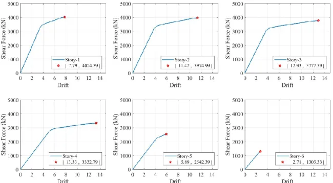
Figure 3.6. Total shear capacity per layer of MF and BF building ... 42

Figure 3.7. The total stiffness of MF and BF building in any stories ... 44

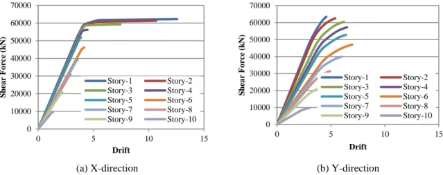
Figure 3.8. The capacity curve of MF structure in X-direction and Y-direction ... 47

Figure 3.9. The capacity curve of MF building for any stories in X-direction ... 48

Figure 3.10. The capacity curve of MF building for any stories in Y-direction ... 48

Figure 3.11. The capacity curve of BF structure in X-direction and Y-direction ... 49

Figure 3.12. The capacity curve of BF building for any stories in X-direction ... 50

Figure 3.13. The capacity curve of BF building for any stories in Y-direction ... 50

Figure 3.14. The mode shape displacement of MF building in both direction ... 51

(8)

vii

Figure 3.15. The mode shape displacement of BF building in both direction ... 52

Figure 3.16. Simulated spectrum acceleration ... 53

Figure 3.17. Maximum response of MF building ... 54

Figure 3.18. Nonlinear dynamic response due to El Centro earthquake of MF building in X- direction ... 55

Figure 3.19. Nonlinear dynamic response due to Kobe earthquake of MF building in X-direction ... 55

Figure 3.20. Nonlinear dynamic response due to Taft earthquake of MF building in X-direction ... 56

Figure 3.21. Nonlinear dynamic response due to El Centro earthquake of MF building in Y- direction ... 56

Figure 3.22. Nonlinear dynamic response due to Kobe earthquake of MF building in Y-direction ... 57

Figure 3.23. Nonlinear dynamic response due to Taft earthquake of MF building in Y-direction ... 57

Figure 3.24. Maximum response of BF building ... 58

Figure 3.25. Nonlinear dynamic response due to El Centro earthquake of BF building in X- direction ... 59

Figure 3.26. Nonlinear dynamic response due to Kobe earthquake of BF building in X-direction ... 59

Figure 3.27. Nonlinear dynamic response due to Taft earthquake of BF building in X-direction ... 60

Figure 3.28. Nonlinear dynamic response due to El Centro earthquake of BF building in Y- direction ... 60

Figure 3.29. Nonlinear dynamic response due to Kobe earthquake of BF building in Y-direction ... 61

Figure 3.30. Nonlinear dynamic response due to Taft earthquake of BF building in Y-direction ... 61

Figure 4.2. Converting the capacity curve to be an elastoplastic curve by the constant energy principle ... 67

Figure 4.3. Perspective and plan view of building A. ... 68

Figure 4.4. Perspective and plan view of building B. ... 70

Figure 4.5. Seismic index of building A and B ... 73

Figure 4.6. Seismic index (Is) of building A and B ... 75

Figure 4.7. Performance point of Building A and B ... 76

Figure 5.1. SDOF system with bilinear hysteretic model ... 79

Figure 5.2. The design response spectrum of Indonesian code ... 82

Figure 5.3. Simulation of the acceleration response spectrum ... 84

Figure 5.4. Relationship between shear force coefficient C and ductility factor μ ... 85

Figure 5.5. Characteristics of maximum displacement ... 86

Figure 5.6. The spectrum of the dynamic seismic index (dIs) ... 89

Figure 5.7. Relationship dynamic ductility index (dF) and critical ductility (cr) ... 90

Figure 5.8. Spectrum of dynamic ductility index (dF)... 91

Figure 5.9. Relationship dynamic ductility index and estimation ductility index ... 92

Figure 5.10. Relationship ductility factor and dynamic ductility index on several estimation methods ... 94

(9)

viii

List of Tables

Table 2.1. Hazard intensity based on spectral acceleration ... 11

Table 2.2. The basic score of all buildings type ... 11

Table 2.3. Score modifier for concrete moment-resisting frame buildings ... 12

Table 2.4. Values of site coefficient Fa as a function of site class and mapped spectral response acceleration at short periods, SS ... 19

Table 2.5. Values of site coefficient Fv as a function of site class and mapped spectral response acceleration at 1.0 period, S1 ... 19

Table 2.6. Importance factors by risk category of buildings ... 21

Table 2.7. Coefficient for the upper limit on the calculated period ... 21

Table 2.8. The building list as cases study ... 26

Table 2.9. The screening checklist ... 27

Table 2.10. The rapid visual screening result ... 28

Table 2.11. Roof drift ratio... 31

Table 3.1. Summarize section property in the 6^th story structure. ... 40

Table 3.2. Summarize section property in the 10^th story structure. ... 40

Table 3.3. Basic configuration evaluation of building A (MF) and building B (BF) ... 43

Table 3.4. Structural evaluation of the moment frame (MF) structure ... 45

Table 3.5. Structural evaluation of the brace frame (BF) structure ... 46

Table 3.6. Ductility factor in any stories of MF building ... 47

Table 3.7. Ductility factor in any stories of BF building ... 49

Table 3.8. Dynamic properties of MF building ... 51

Table 3.9. Dynamic properties of BF building ... 52

Table 3.10. Simulated earthquake ground motions ... 53

Table 4.1. Material properties of building A and B ... 69

Table 4.2. Beam and column dimension of the building A ... 69

Table 4.3. Beam and column dimension of the building B ... 70

Table 4.4. Seismic index of building A ... 72

Table 4.5. Seismic index of building B ... 72

Table 4.6. The lateral force in building A and B ... 73

Table 4.7. The capacity curve of building A and building B ... 74

Table 4.8. Seismic index using pushover analysis ... 75

Table 4.9. Seismic index comparison ... 76

Table 4.10. Evaluation of the structure performance ... 77

Table 5.1. Selected ductility factor when varying T0 and Cy ... 81

Table 5.2. Simulated earthquake ground motions ... 83

Table 5.3. The shear coefficient of C0 ... 88

Table 5.4. The percentage of error estimation for each dF estimation ... 93

Table 5.5. The percentage of error comparison for both estimation method ... 95

(10)

ix

Abbreviations

AIJ Architectural Institute of Japan

AISC American Institute of Steel Construction ASCE American Society of Civil Engineering

ATC Applied Technology Council.

BF Brace Frame

BSL Building Standard Law

CM Center of Mass of the story CR Center of Rigidity of the story

CSM Capacity Spectrum Method

DBE Design Basis Earthquake

ELM Equivalent Linearization Method

FEMA The Federal Emergency Management Agency

IBC International Building Code

JBDPA The Japan Building Disaster Prevention Association MCE Maximum Considered Earthquke Ground Motion

MDOF Multi Degree of Freedom

MF Moment Frame

MRF Moment Resisting Frame

NEHRP National Earthquake Hazard Reduction

PGA Peak Ground Acceleration

RVS Rapid Visual Screening

REM Rapid Evaluation Method

SCWB Strong Column Weak Beam

SDOF Single Degree of Freedom

SMF Special Moment Frame

SIMEQ Simulated of Earthquake ground motion

(11)

1

Chapter 1

Introduction

1.1. Background

Over the past 50 years, Indonesia has often suffered major damaging earthquakes. It is difficult to precisely estimate the magnitude and number of earthquakes that will occur during the life of a building. There are still thousands of buildings in earthquake-prone regions that require seismic evaluation and rehabilitation [1]. A series of earthquake events have occurred in Indonesia in the past.

The most recent earthquakes located along the Sumatran-Andaman plate was in 1797 with the magnitude in between 8.7 - 8.9. In 2004, The great earthquake of magnitude 9.1 and immediately following by devastating tsunami occurred in Simeulue Island of Banda Aceh. There was an earthquake in September 2007 of magnitude 8.5 in Mentawai island. A magnitude of 7.6 due to the subducting plate caused considerable damage in Padang in 2009 and a magnitude of 7.8 in 2010 again occurred in the Mentawai island caused a tsunami on the west coast of those islands [2, 3]. The historical earthquake epicenter can be seen in Figure 1.1.

In recent years, the earthquake resistance structure design has experienced changes significantly because of the increased demand for enhancement of structural capacity in order to minimize the level of damage, economic loss, and structure repair costs. Several researchers have been studied the seismic hazard of Indonesia and the earthquake-resistant standard design for the building. Asrurifak et al., 2010, studied in updating the spectral hazard map of Indonesia with a return period of 2500 years earthquake. The spectral hazard map was analyzed using the total probability method and three- dimensional source models with recent seismotectonic parameters. Four source models were used in

(12)

2 this analysis: shallow background, deep background, fault, and subduction source models. This study proposed the revision of the Indonesia hazard map by referring to International Building Code (IBC) where spectral acceleration values at peak ground acceleration, at 0.2 seconds and at 1.0 seconds were applied for general buildings with a return period of 2500 year. Generally, the results of the analysis show the values of PGA with a return period of 2500 years relatively higher 1.2-3.0 times than in Indonesia seismic code at that time [4].

Figure 1.1. The historical of earthquake epicenter in Indonesia [5]

Irsyam et al., 2017, presents the progress in developing Indonesia seismic hazard maps. The revision of seismic hazard maps has been developed based upon updated: seismotectonic data, fault models, and attenuation function. Important information is considered for updating seismic hazard maps such as significant results of recent active-fault studies utilizing trenching, carbon dating, epicenter relocation, strain analysis as well as the availability of the recently available data. The new information was gathered in order to obtain a more accurate tectonic model and their seismic parameters, such as maximum magnitudes and slip-rates. Finally, probabilistic and deterministic analyses were then performed in order to develop new seismic hazard maps [3].

The earthquake resistance design code for building in Indonesia has been updated from time to time to minimize risk and human life fatalities. Figure 1.2 shows the historical of the seismic hazard map of Indonesia, and consequently the seismic load demand also increases. The existing buildings

(13)

3 may not comply with the requirements of the current code anymore. It needed evaluation to show the performance against the current code. Several evaluation methods can be used to evaluate existing buildings. The nonlinear analysis is a reliable method to confirm existing structural performance.

However, a large number of buildings in Indonesia makes it difficult to carry out detailed structural evaluations. The tons of buildings in a city need a rapid method to conduct an evaluation.

Figure 1.2. The history of the seismic hazard map of Indonesia [6]

Nakazawa et al. have been conducted several researches to evaluate the existing structure performance in Japan. In 2011, Nakazawa has been studied evaluation of dynamic ductility index of a school gymnasium [7]. The paper discussed the seismic resistance capacity of the school gymnasium subjected to earthquake motions in the span direction. Based on the result of the elasto-plasitc dynamic analysis depending on various input levels, the values of dIs and dF for the gable frame structure were calculated. As numerical parameters, critical plastic rotation, θpcr

, of the gable frame structure was adopted, and the effects on dIs and dF were investigated. Two kinds of fundamental gable frames, Frames A and B, were studied. The results show that the skeleton curves of Frame A and B became tri-linear and bi-linear types, respectively. Plastic rotation θp of Frame A was greatly large compared with θp of Frame B. Therefore, the energy absorption performance of Frame B was superior to that of

(14)

4 Frame A. Criteria of plastic angle θpcr were assumed to be 0.005, 0.01, 0.02, 0.03, 0.04 and 0.05. The

dIs and dF became large with the increase in θpcr. The dF of Frame A was distributed from 0.71 to 1.82 and dIs was distributed from 0.28 to 0.72. The dF of Frame B was distributed from 1.40 to 4.89 and dIs

was distributed from 0.76 to 2.66. In 2013, Nakazawa has been studied a method of evaluation for Japan’s steel gymnasium with the dynamic structural seismic index and dynamic ductility index based on pushover analysis [8]. The resistance capacity subjected to horizontal seismic motions in the span direction was investigated. The correspondence of the time history analysis and pushover analysis based on a capacity spectrum method was studied in detail with respect to some adjustment factors to increase accuracy. The proposed pushover analysis using some adjustment factors proved as a design tool for evaluating the important seismic index. In 2017, Nakazawa proposed an estimation method of the dynamic ductility index using the equivalent linearization method (ELM) [9]. The ELM expresses a system with nonlinear restoring force as a linear system with equivalent stiffness and equivalent damping factor. The equivalent stiffness, keq, is defined as the maximum shear force divided by the maximum point stiffness. Further, the equivalent natural period, Teq, corresponding to the equivalent stiffness, can also be obtained. The equivalent linearization method is a simple method for estimating the ductility index without conducted a nonlinear dynamic analysis. The dynamic structural seismic index was determined with corresponding to the critical deformation of a member. A steel gymnasium supported by a substructure was use as a case study and it modeled as a single degree of freedom (SDOF) system when the rigidity of the upper roof structure assumed quite high. The validity of the proposed estimation method show good accuracy in estimating the index.

1.2. Research Objective

The purpose of this study is to develop a systematic evaluation of the performance of existing buildings in resilience to face major earthquakes that may occur in the future and can also measure how much the lack of performance of existing buildings against the update code that currently apply.

This study takes several cases of the existing building in Pekanbaru and Padang city of Indonesia in collecting building information. Various structural types and building occupancies in these two cities are the objects of this study. Therefore, this study aims as follow:

1. To learn the possibility of a rapid evaluation method as the initial screening procedure that can be carried out in a short time, taking into consideration the large number of buildings to be assessed.

(15)

5 2. To investigate a further rapid evaluation by examining the general aspects of building and the

characteristic of the structural system and geological information.

3. To formulate an index to measure the level of the existing building performance and estimate the level of safety by comparing to the demand hazard in a certain location.

4. To investigate the actual of the existing building performance with reliable methods such as static and dynamic nonlinear analysis guide in considering the accuracy of the proposed evaluation method.

1.3. Thesis Outline

This thesis will be outlined as follow. Chapter 1 is an introduction that describes the background of this study and the research objective. Then, chapter 2 will describe the application of the Rapid Visual Screening (RVS) method in the Pekanbaru city of Indonesia. The selected 15 buildings as case studies were investigated. The result is then confirmed with a static pushover analysis method and describing reliability that this method can be used as a preliminary evaluation. The next chapter, chapter 3, will represent the Rapid Evaluation Method (REM) which is a further screening evaluation to investigate the structure configuration and the element component for resisting an earthquake load.

The REM is developed in the two of the checklists procedure: the configuration structure checklist and the element for resisting the earthquake load checklist. In this chapter, the case study is selected for the steel structure in differing structural systems. Afterward, chapter 4 will be a chapter about a method of calculation of a seismic index with the pushover analysis method. The seismic index is an index to describe the performance of the existing building which is popular in Japan. The safety limit of the seismic index called a seismic demand index is proposed by considering Indonesia's seismic hazard which is defined in the current seismic code in Indonesia. The last chapter, chapter 5, describes the conclusion of this thesis.

(16)

6

Chapter 2

Structural Building Screening with Rapid Visual Screening (RVS)

2.1. Introduction

An earthquake is a sudden shift from soil layers due to the movement of the earth's surface. The shift creates a vibration called seismic waves. An earthquake will shake building in horizontally and vertically. The vertical forces rarely make structural collapse, but the horizontal force potentially makes it as long as this force exceeds the capacity of the structure. An earthquake is a disaster that can be harmful to the community, such as financial loss and loss of human life. Pekanbaru is a city which is located in the middle of Sumatera Island. Even though Pekanbaru is a rarely occurring earthquake, but Pekanbaru has ever felt the impact of a big earthquake that occurred in West Sumatera in September 2009. As we know, Indonesia located between the Eurasian plate, Pacific plate and Indo- Australian plate. Particularly the Sumatera Island, which has the Semangko fault or the great Sumatra fault along the island from north to south due to shift of Eurasian and Indo-Australian Plates. An earthquake is not killing people but the collapse of building around the people could be killing them.

Generally, before building constructed there was the structural design which established with certain earthquake loads comply to a standard, but for the existing of the buildings which have a lack of the standard design and inadequate structure capacity to resist earthquake load has become a serious problem. Since 2012, there was a new code for the design of earthquake resistance in Indonesia, namely “The design procedures of the earthquake resistance for building and non-building structures”

[10]. This was a revision and updated of the previous code that has been released since 2002. Figure

(17)

7 2.1 shows the comparison of seismic maps of Pekanbaru city based on before and after updated code [10, 11]. The preventive action to avoid the damage of the building will become severe damage should be taken into consideration. There are various evaluation methods to anticipate the building in severe damage when hit by an earthquake. One of the methods is a performance base evaluation. The performance base evaluation can provide sufficient information to what extent the earthquake will affect the structure of the building [12].

(a) (b)

Figure 2.1. Seismic map of Pekanbaru city of Indonesia

(a). Indonesia code SNI 03-1726-2002 [13] (b). Indonesia code SNI 1726:2012 [10]

The objective of this research is to make an assessment of the existing building and to conduct evaluation using rapid visual screening method in order to get further consideration against the earthquake load. Non linear static analysis is used as a comparison. Therefore the result provide recommendations for the facility owner about their building condition and taking preventive action against inadequate resistance due to an earthquake load.

2.2. Methodology

A methodology for assessing building vulnerability is needed. A screening procedure in the initial stage of evaluation useful for a large number of building population. The screening procedure issued by the Federal Emergency Management Agency (FEMA) will be studied in this research. The FEMA 154 introduces screening evaluation of the existing structure. Several buildings were selected in Pekanbaru city and it will be evaluated by using these methods.

Ramly et al. conducted a seismic assessment of existing buildings in Bukit Tinggi in Pahang of Malaysia [14]. Six general building occupancies that are easy to recognize have been defined. These are listed on the data collection form as residential, commercial, industrial, educational, government, assembly, history and emergency services. A total of 1166 were identified in Bukit Tinggi. The highest occupancy class is residential as much as 84 percent. The results of preliminary visual

(18)

8 inspection were completed for these buildings. A total of 26 percent of the buildings indicated that the buildings need to be further evaluated by the professionals based on engineering practice because the buildings have a probability of damage due to ground motion activity. Whereas, another 74 percent of buildings are safe from the ground motion. The results revealed that the score determined for the factor of primary structural lateral load resisting system (building types), has the highest contribution to the final score of the buildings. Other than that, most of the multi-story buildings have a soft story which is a large opening at the ground level commonly for parking areas. The buildings in Bukit Tinggi are on a steep hill so that over the up-slope dimension of the building the hill raises at least one story height. A problem may exist because along the lower side of the story, the horizontal stiffness may be different from the uphill side. Additionally, the stiff short columns attract the seismic shear forces and may fail. These contribute to the reduction of the final score due to the vertical irregularity.

M. Syah et al. used the RVS method to determine the vulnerability of buildings in two districts of Jeddah Saudi Arabia [15]. The screening evaluation was performed on over 1000 residential buildings structures in two different time periods with an aim to evaluate the differences between older and recent buildings in a rapidly-expanding city of Saudi Arabia. Results of the visual screening were consistent and reasonable considering the age of buildings based on the data obtained previously.

Results of the visual screening were consistent and reasonable considering the age of buildings based on the data obtained previously. Upon the results of the investigation, the used typical structure and state of the buildings can be determined. A clear distinction can be made concerning the different age of the building resulting in different structures. Residential buildings in Al-Balad district are old and buildings in As-Salamah district were built recently based on new seismic codes. This information allows the furthermore detailed seismic analysis of existing buildings.

2.3. Rapid Visual Screening

Rapid Visual Screening (RVS) is a fast method to identify a risk of building and it can be conducted without performing any structural analysis. Buildings are rapidly evaluated via a “sidewalk survey” to identify features that affect the seismic performance of the building. Many of the RVS methods have been developed in the worldwide [16–18]. According to the difference in building codes and construction practices, the scoring system and parameters are taken for assessing the vulnerability of buildings that differ from place to place. One of the methods and scoring systems for rapid screening was developed by FEMA [4] . The results can be used as guidance to make consideration for the next action. If the results indicate that the building does not meet the requirements, then the

(19)

9 next action will be evaluated by the detailed evaluation before making a final decision for retrofitting or demolishing. The RVS method is carried out by filling the form as shown in Figure 2.2. Various features were considered during this procedure. These features may include building type, seismicity, soil conditions and irregularities. The inspection, data collection and decision-making process typically occurs at the building site, and is expected to take around 20 min for each building [19].

Figure 2.2. The complete form of the RVS

(20)

10 The RVS form as shown in Figure 2.2 consist of several sections. On the top left of this sheet, it is for illustrating a sketch of a building structure. And following in the top right is for the detail of identification of the building location. The building image can also be attached in the middle of this sheet. The occupancy criteria, soil type and the potential falling hazard can be described in the middle of this sheet as zoom in Figure 2.3 (a),(b) and (c) respectively. The main part of this sheet is in the determination of basic score and score modifier in next to the middle of this sheet. FEMA 154 assigns a basic structural score based on seismic hazard intensity of the region, building type and lateral load resisting system of the building. Performance modifiers are specified to take into account the effect of a number of stories, plan and vertical irregularities, pre-code or post-benchmark code detailing, poor condition of the building and type of soil.

There are several types of structure base on composing material including wood, steel, concrete, prestressed concrete and unreinforced masonry. Each type of structure has a different basic score as shown in Figure 2.3 (d) and it describes in Table 2.2.

(a) Building categories and Occupancy

(b) Soil Type (c) Potential Falling hazard.

(d) Basic score and score modifiers

Figure 2.3. Section description in the RVS form

(21)

11 Table 2.1. Hazard intensity based on spectral acceleration

Level of seismic hazard intensity

Calculated 2/3 SA for a period of 0.2 second (or SDS)

Calculated 2/3 SA for a period of 1.0 second (or SD1)

Low Less than 0.167 g Less than 0.067 g

Moderate Greater than or equal to 0.167 g but less than 0.5 g

Greater than or equal to 0.067 g but less than 0.2 g High Greater than or equal to

0.5 g

Greater than or equal to 0.2 g

The basic score as shown in Table 2.2 classified in three-level seismic intensities consists of high hazard intensity; moderate hazard intensity ; low hazard intensity. The higher the seismicity level will be the lower of the basic score.

Table 2.2. The basic score of all buildings type

Building Type Seismicity

Low Moderate High Lightwood frame single or multiple

family dwelling of one or more stories in height

(W1) 7.4 5.2 4.4

Wood frame commercial and industrial buildings with a floor area larger than 5,000 square feet

(W2) 6.0 4.8 3.8

Steel moment-resisting frame buildings (S1) 4.6 3.6 2.8

Braced steel frame buildings (S2) 4.8 3.8 3.0

Light metal buildings (S3) 4.6 3.8 3.2

Steel frame buildings with concrete shear walls

(S4) 4.8 3.6 2.8

Steel frame buildings with unreinforced masonry infill walls

(S5) 5.0 3.6 2.0

Concrete moment-resisting frame buildings

(C1) 4.4 3.0 2.5

Concrete shear wall buildings (C2) 4.8 3.6 2.8

Concrete frame buildings with unreinforced masonry infill walls

(C3) 4.4 3.2 1.6

Tilt-up buildings (PC1) 4.4 3.2 2.6

Precast concrete frame buildings (PC2) 4.6 3.2 2.4

Reinforced masonry buildings with flexible floor and roof diaphragms

(RM1) 4.8 3.6 2.8

Reinforced masonry buildings with rigid floor and roof diaphragms

(RM2) 4.6 3.4 2.8

Unreinforced masonry bearing-wall buildings

(URM) 4.6 3.4 1.8

(22)

12 The hazard Intensity is part of the Rapid Visual Screening forms since the vulnerability of existing buildings is related to the intensity of the earthquake hazard, greater the intensity higher the damage the building will sustain and higher will be its vulnerability. Hence each level of seismic intensity forms the basis of one Rapid Visual Screening Form and the number of such forms will be equal to the number of seismic intensity zones. According to FEMA 154 (2002), the level of hazard intensity will be determined in the following manner. From the seismic hazard map of the country, find the spectral accelerations design (SA) for a natural period of 0.2 seconds and 1.0 seconds, then multiply the value by a factor of 2/3 and check the calculated values as in Table 2.1.

The basic score of the selected building type will be modified with several score modifiers as shown in Table 2.3. The score modifier can be a positive value that will be added to the basic score otherwise it can be a negative value that will be deducted the basic score.

Table 2.3. Score modifier for concrete moment-resisting frame buildings Seismicity

Low Moderate High Mid Rise (4 to 7 stories) 0.4 0.2 0.4

High Rise (> 7 stories) 1.0 0.5 0.6 Vertical Irregularity -1.5 -2.0 -1.5

Plan Irregularity -0.8 -0.5 -0.5

Pre - Code N/A -1.0 -1.2

Post- Benchmark 0.6 1.2 1.4

Stiff Soil (Type D) -0.6 -0.6 -0.4

Soft Soil (Type E) -1.4 -1.0 -0.6

Poor Soil (Type F) -2.0 -1.6 -1.2

The use of the RVS which is expected to have acceptable seismic performance should establish an appropriate score call as a “cut-off” score. A score of 2 is suggested as a “cut-off “ base on seismic design criteria. A building having a score of 2 or less should be investigated by further detail evaluation.

2.3.1. Number of Stories

From Table 2.3, the top two modifiers are related to a number of stories. The basic score will be modified with a positive value of a modifier score. If the building has 4 to 7 stories, it is considered a mid-rise building, and the positive score modifier associated with this attribute should be circled. If the building has 8 or more stories, it is considered a high-rise building, and the score modifier associated

(23)

13 with this attribute should be circled. The high-rise building has a score modifier higher than the mid- rise building.

2.3.2. Vertical Irregularity

If a structure has vertical irregularity, the score modifier will be deducted from the basic score.

The amount of a modifier varies in range -1.5 until -4.0 for all types of buildings. Examples of vertical irregularity include buildings with setbacks, hillside buildings, and buildings with soft stories (see illustrations of potential vertical irregularities in Figure 2.4). If the building is irregularly shaped in elevation, or if some walls are not vertical, then apply the modifier. If the building is on a steep hill so that over the up-slope dimension of the building the hill rises at least one story height, a problem may exist because the horizontal stiffness along the lower side may be different from the uphill side. In addition, in the up-slope direction, the stiff short columns attract the seismic shear forces and may fail.

In this case the performance modifier is applicable.

Figure 2.4. The irregularities potential in a vertical direction [16]

A soft-story exists if the stiffness of one story is dramatically less than that of most of the others such as shear walls or infill walls not continuous to the foundation. Soft stories are difficult to verify without knowledge of how the building was designed and how the lateral forces are to be transferred from story to story. There may be shear walls in the building that are not visible from the street.

However, if there is a doubt, it is best to be conservative and indicate the existence of a soft story by circling the vertical irregularity score modifier. Use an asterisk and the comment section to explain the source of uncertainty. In many commercial buildings, the first story is soft due to large window openings for display purposes. If one story is particularly tall or has windows on all sides, and if the stories above have a few windows, then it is probably a soft story. A building may be adequate in one direction but be “soft” in the perpendicular direction. For example, the front and back walls may be open but the sidewalls may be solid. Another common example of a soft story is pilotis building.

(24)

14 Several past earthquakes have shown the vulnerability of this type of construction. Vertical irregularity is a difficult characteristic to define, and considerable judgment and experience are required for identification purposes.

2.3.3. Plan Irregularity

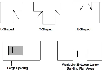
Plan irregularity is one of the criteria for modifying score and it can affect all building types. If a structure has this kind of irregularity, the score modifier will be deducted from the basic score. The amount of a modifier is -0.8 for low seismicity and -0.5 for moderate and high seismicity. Examples of plan irregularity include buildings with re-entrant corners, where damage is likely to occur; buildings with good lateral-load resistance in one direction but not in the other; and buildings with major stiffness eccentricities in the lateral force-resisting system, which may cause twisting (torsion) around a vertical axis.

Figure 2.5. Plan views of various building configurations showing plan irregularities;

arrows indicate possible areas of damage.

Buildings with re-entrant corners include those with long wings that are E, L, T, U, or + shaped (see Figures 2.5). Plan irregularities causing torsion are especially prevalent among corner buildings, in which the two adjacent street sides of the building are largely windowed and open, whereas the other two sides are generally solid. Although plan irregularity can occur in all building types, the primary concern lies with wood, tilt-up, pre-cast frame, reinforced masonry and unreinforced masonry construction. Damage at connections may significantly reduce the capacity of a vertical-load-carrying element, leading to partial or total collapse.

(25)

15 2.3.4. Post-Benchmark

The post-benchmark score modifier is applicable if the building being screened was designed and constructed after significantly improved seismic codes applicable were adopted and enforced by the local jurisdiction. In high and moderate seismicity regions, the basic structural hazard scores for the various building types are calculated for buildings built after the initial adoption of seismic codes, but before substantially improved codes were adopted. For these regions, score modifiers designated as

“Pre Code” and “Post Benchmark” are provided, respectively, for buildings built before the adoption of codes and for buildings built after the adoption of substantially improved codes. In low seismicity regions, the basic structural hazard scores are calculated for buildings built before the initial adoption of seismic codes. for buildings in these regions, the score modifier designated as “Pre Code” is not applicable (N/A), and the Score Modifier designated as “Post Benchmark” is applicable for buildings built after the adoption of seismic codes.

In the case of the post-benchmark in this study, a justification was proposed and used to apply RVS for Indonesian conditions. Indonesia seismic code was first introduced in 1966 and then updated several times in 1983, 2002 and recently in 2012. The 1983 seismic code has significant changes compared with previous code, therefore this year is used as a post benchmark in studies this. Buildings built in 1983 and above are considered adding a score modifier so that the post-benchmark is chosen.

Otherwise the building constructed under 1983 is simulated by reducing the score modifier by selecting the pre-code.

2.3.5. Soil Type

Soil type has a major influence on amplitude and duration of shaking, and thus structural damage.

The six soil types considered in the RVS procedure: hard rock (type A); average rock (type B); dense soil (type C), stiff soil (type D); soft soil (type E), and poor soil (type F). A shear wave velocity (Vs) is a parameter to determine the classification of soil type. Score Modifiers are provided for soil type C, Type D, and Type E. The appropriate modifier should be circled if one of these soil types exists at the site. If sufficient guidance or data are not available during the planning stage to classify the soil type as A through E, a soil type E should be assumed. However, if the actual site conditions are not known for one- or two-story buildings with a roof height equal to or less than 25 feet (or 7.5 m), a class D soil type may be assumed. There is no score modifier for Type F soil because buildings on soil type F

(26)

16 cannot be screened effectively by the RVS procedure. A geotechnical engineer is required to confirm the soil type F and an experienced professional engineer is required for building evaluation.

2.4. Indonesian Code for Earthquake Resistance Building Design

As mentioned in the introduction, the design of Indonesian building codes has undergone several changes since it was first developed in 1966. The most current code still in effect today is SNI 1726- 2012. The objective of the building code philosophy for seismic design is to prevent collapse in the extreme earthquake likely to occur at a building site. Seismic criteria adopted by current model codes involve a two-level approach to seismic hazard, which are the design bases earthquake (DBE) and maximum considered earthquake (MCE). DBE’s ground motion has a 10% probability of being exceeded in 50 years (475 year-return period earthquake). The DBE is the design-basis earthquake for conventional building design, with margins provided by the inherent conservatism built into the NEHRP (National Earthquake Hazard Reduction) 1997 Provisions. The ground motion at the DBE level is defined as being two-thirds of the MCE as follow,

2

DBE = 3 MCE ... (2.1)

The MCE ground motions are defined as the maximum level of earthquake shaking that is considered reasonable to design a normal structure to resist or the worst-case scenario of an earthquake to be expected. The MCE ground motion is taken as 2% probability of being exceeded in 50 years (2500-year return period earthquake). It is implied that the design in the MCE shaking level has a target performance of near to collapse.

Procedure to determine response spectral design at MCE’s condition consider the following parameters,

1) Site coefficient corresponding to a short period (Fa) 2) Site coefficient corresponding to the 1.0 second period (Fv)

3) Mapped spectral response acceleration of MCE ground motion at a short period (Ss) 4) Mapped spectral response acceleration of MCE ground motion at the 1.0 second period (S1) 5) Spectral coefficient at a short period (SMS)

6) Spectral coefficient at the 1.0 second period (SM1)

7) Spectral coefficient of DBE ground motion at a short period (SDS) 8) Spectral coefficient of DBE ground motion at the 1.0 second period (SD1) 9) Fundamental of period (T)

(27)

17 2.4.1. Seismic Ground Motion Maps

In Indonesian Code, SNI 1726-2012, the 5% damped response spectra are constructed from the mapped maximum considered earthquake spectral response at two points. The 1^st point denoted as SS, corresponds to short periods, and the second point denoted as S1 corresponds to the 1.0 second period.

Maps for Indonesia seismic intensity have been developed and are shown in Figure 2.6 and 2.7. From the first map, the mapped risk target maximum considered earthquake (MCER) spectral response acceleration for a short period, SS, is found based on the location of the site. The second map is used to determine the mapped MCER spectral response acceleration for a 1.0 second period, S1.

Figure 2.6. SS , Risk-adjusted maximum considered earthquake (MCER) ground motion parameter for Indonesia for 0.2s spectral response acceleration (5% of critical damping) [10]

(28)

18 Figure 2.7. S1 , Risk-adjusted maximum considered earthquake (MCER) ground motion parameter for

Indonesia for 1.0s spectral response acceleration (5% of critical damping) [10]

2.4.2. Adjustments to Spectral Response for Site Class Effects

The SS and S1 values correspond to a site class B, and adjustments must be made if the site in question is other than a site class of B profile. The SS and S1 values are adjusted for the site effects by the following formulas:

MS a S

S =F S ... (2.2)

1 1

M v

S = F S ... (2.3)

where Fa is a site coefficient for a short period response, and Fv is a site coefficient for 1 second period response. SMS and SM1 are the 5% damped spectral response acceleration of MCE at short and 1.0 second periods, respectively. The values of Fa and Fv are defined by both the local soil condition and the values of SS and S1 by using Table 2.4 and Table 2.5.

In Table 2.4 and Table 2.5, Site Class represents a soil condition that consists of 5 classes. Site Class A, B, C, D, and E, which classify as Hard rock, Rock, Dense Soil, Stiff soil and Soft Soil, respectively. The site coefficient seems to increases with the softening of the soil and decrease with decreasing the response acceleretion.

(29)

19 Table 2.4. Values of site coefficient Fa as a function of site class and mapped spectral response

acceleration at short periods, SS

Site Class

Mapped Spectral Response Acceleration at Short Periods

SS ≤ 0.25 SS = 0.5 SS = 0.75 SS = 1.0 SS ≥ 1.25

A 0.8 0.8 0.8 0.8 0.8

B 1.0 1.0 1.0 1.0 1.0

C 1.2 1.2 1.1 1.0 1.0

D 1.6 1.4 1.2 1.1 1.0

E 2.5 1.7 1.2 0.9 0.9

A = Hard rock, B = Rock, C = Dense soil, D = Stiff soil, E =Soft soil

Note: Use straight-line interpolation for intermediate values of mapped spectral acceleration at short periods, SS.

Table 2.5. Values of site coefficient Fv as a function of site class and mapped spectral response acceleration at 1.0 period, S1

Site Class

Mapped Spectral Response Acceleration at 1 second Period

S1 ≤ 0.1 S1 = 0.2 S1 = 0.3 S1 = 0.4 S1 ≥ 0.5

A 0.8 0.8 0.8 0.8 0.8

B 1.0 1.0 1.0 1.0 1.0

C 1.7 1.6 1.5 1.4 1.3

D 2.4 2.0 1.8 1.6 1.5

E 3.5 3.2 2.8 2.4 2.4

A = Hard rock, B = Rock, C = Dense soil, D = Stiff soil, E =Soft soil

Note: Use straight-line interpolation for intermediate values of mapped spectral acceleration at 1.0 periods, S1.

2.4.3. General Design Response Spectrum

To determine the general design response spectrum with 5% damping, two quantities, the 5% damped design spectral response acceleration at short periods, SDS, and at 1-second periods, SD1, are determined by the following equations:

2

DS 3 MS

S = S

1 1

2

D 3 M

S = S ... (2.4)

(30)

20 General design response spectrum SA0(T) as a demand acceleration response spectrum with 5%

damping of Indonesian code is obtained by the following equation,

0 0

1

0.4 0.6 ...

( ) = ...

...

DS

A DS S

D

S

S T T T

T

S T S T T T

S T T

T

  

+ 

  

 

  



 

 . ... (2.5) where, ₀ = 0.2 ^D¹ , _S = ^D¹

DS DS

S S

T T

S S

The T0 and Ts is a range of period where the acceleration response has a constant value equal to SDS.

Figure 2.8 shows the design response spectrum, Design Bases Earthquake (DBE) ground motions, as it conforms to Indonesian code SNI 1726-2012 [10].

Figure 2.8. General design response spectrum with 5% damping [10]

2.4.4. Seismic Response Coefficient

Seismic base shear, V, in a given direction is obtained by a seismic response coefficient (CS) and the weight of a structure (W) with the following equation:

V =C WS ... (2.6)

The seismic response coefficient, CS, can be determined with considering SDS , a response modification factor (R) and an Importance factor (Ie) as follow:

DS S

e

C S R I

=  

  

... (2.7) SDS

1

SD

T0 T_s 1.0 T (second)

Spectral Acceleration (g)

1

SD

T

0.4S_DS

(31)

21 The value of CS computed with Eq. 2.7 should not be less than 0.01 or 0.5 ¹

( / _e) S R I

 when S1  0.6 (g).

The response modification response, R, depends on structural material and the structural system. In general, R is in the range of 2.0 to 8.0. The structure that has high ductility will have a high R value.

The importance factor focus on earthquake cause, Ie, depends on a risk factor categorizing from level I until IV and bulding occupancy. The high risk will have a hight important factor, as shown in Table 2.6. The building occupancy generally is is risk category II or III.

Table 2.6. Importance factors by risk category of buildings Risk

Category

Seismic Importance Factor (Ie)

Building Occupancy

I 1.00 Low risk to human life in the event of failure

II 1.00 Except those listed in Risk Categories I, III, and IV III 1.25 Substantial risk to human life in the event of failure,

not included in Risk Category IV

IV 1.50 Essential facilities such as: Fire station, Hospital, Power station (including, but not limited to, facilities that manufacture, process, handle, store, use, or dispose of such substances as hazardous fuels,

hazardous chemicals, or hazardous waste)

A fundamental period of the structure, T, is established using the structural properties and deformational characteristics in a proper analysis. In the preliminary analysis, it begins with approximating the fundamental period (Ta). The approximate fundamental period, for structure not exceeding 12 stories could be obtained by the following equation,

a 0.1

T = N ... (2.8) in which N is the number of stories above the base.

The fundamental period shall not exceed the upper limit of period Cu.Ta , where Cu is an upper limit coefficient. The upper limit coefficient depends on the design spectral acceleration of SD1. Table 2.7 shows the list of the upper limit coefficient.

Table 2.7. Coefficient for the upper limit on the calculated period Design spectral acceleration of SD1 Coefficient Cu

 0.4 1.4

0.3 1.4

0.2 1.5

0.15 1.6

 0.1 1.7

(32)

22 2.5. Static Nonlinear

The static nonlinear analysis method is used to confirm the existing building condition in this study. The method is also known as pushover analysis, which is to analyze the capacity of a structure until a collapsed state of the structure is reached [20–25]. When a structure is subjected to gravity loading, a monotonic lateral load is applied and continuously increased with an incremental load through elastic and inelastic behavior until an ultimate condition. The lateral load represents a range of base shear induced by earthquake loading, and its configuration is proportional to the distribution of mass along with building height or mode shapes. The output will generate a capacity curve that plots a strength-based parameter against deflection. In general, the load magnification factor in a step is given for a certain value, and then it is calculated to obtain an incremental displacement of a certain node.

When analyzing frame objects, material nonlinearity is assigned to discrete hinge locations where plastic rotation occurs [26–28]. Beam and column components are modeled as nonlinear frame elements by defining plastic hinges at both ends of the elements. As shown in Figure 2.9, The plastic hinges properties have five points labeled A, B, C, D, and E, which defined the force-deformation behavior. The same type of curve is also used for moment and rotation relationship. The value assigned to each of these points varies depending on the type element, material properties, and section size.

Figure 2.9. Moment-rotation relationship of typical plastic hinge

A linear response is related to a line between point A and an effective yield point B. The slope from point B to point C is typically a small percentage (0% to 10%) of the elastic slope and is included to represent phenomena such as strain hardening. Point C has an ordinate that represents the strength of the element and an abscissa value equal to the deformation at which significant strength degradation begins (line CD). Beyond point D, the element responds with substantially reduced strength until point E. At deformations greater than point E, the seismic element strength is essentially zero [28]. The properties of the plastic hinges for each column and beam are shown in Figure 2.10.