05 -09 , June 2017, Braunschweig, Germany
Identification for input sound pressure level in hammering test based on adjoint variable and finite element methods
Eiki MATSUOKA1, Takahiko KURAHASHI2, Yuki MURAKAMI3, Shigehiro TOYAMA3, Fujio IKEDA3, Tetsuro ITAMA3 and Yoshihiro TAWARA3
1 Nagaoka University of Technology, Niigata, Japan, [email protected]
2 Nagaoka University of Technology, Niigata, Japan, [email protected]
3National Institute of Technology, Nagaoka College, Niigata, Japan
Abstract
In this study, we present the inverse analysis for identification of hammering signal in non-destructive hammering test. The performance function is defined by square sum of residual between the obtained and the computed sound pressure. Here, the problem is to find the input sound pressure so as to minimize the performance function. The formulation for this problem is carried out by the adjoint variable method, and the numerical simulation of the sound pressure propagation is carried out based on the wave equation and the finite element method. As a result of numerical experiments of forward analysis sets to correcting wave of sound pressure in input point of inverse analysis.
Keywords: Non-destructive testing, Hammering test, Wave equation, Finite element method, Adjoint variable method
1. Introduction
Conventionally, if the nondestructive testing is carried out to investigate the reinforcement bar arrangement, methods using the electromagnetic wave radar and the electromagnetic induction are frequently employed in Japan.
However, it is said that the measurement error for the investigation is not small, and it appears that it is necessary to improve the investigation system of the reinforcement bar arrangement. On the other hand, the hammering test is often carried out to investigate the cavity existence in concrete. It is known that this method is employed based on sense by experience for each investigator. In recent years, a research on clustering with respect to the size and the position of the defect in concrete has been carried out based on the frequency response function considering the characteristic of the hammering [1]. The clustering is carried out using the measurement data by hammering and the input signal measured by the “impulse hammer”. However, the hammer is expensive measurement tool, and it is desired that the development of the identification tool of the input sound pressure by the measurement data is performed. Therefore, in this study, the identification of input sound pressure is carried out based on the finite element and the adjoint variable methods. The wave equation is introduced to simulate the propagation of sound pressure in the test piece. The finite element Galerkin procedures is applied to discretize the governing equation in space. In addition, the method proposed by Krenk [2] is employed to discretize the governing equation in time.
2. Formulation for input signal identification problem by adjoint variable method
2.1. Definition of performance function
In this study, sound pressure which is obtained by substituting base sound pressure value in sound pressure level equation applies to performance function. Voltage value measured by microphone convert into sound pressure level. The square residuals sum of the sound pressure value obtained by measure voltage value pobj: and the computational value p defines as performance function shown in Eq. (1),
p p
Q p p
d dtJ obs
t
t obs
f
. .2 0
1 (1)
where tf and Q respectively indicate terminal time of computation and weighting function. The weighting function Q sets 1 on the observation point, and 0 on the others. In this input signal identification problem, we obtain time history of the sound pressure in hammering point whose the minimization of performance function based on wave equation shown Eq. (2), initial condition and boundary condition shown Eqs. (3) - (6),
, 0
2
c pii p
(2)
p at t t in
p ˆ 0 (3)
p at t t in
p ˆ 0 (4)
1
unknown on
p (5)
2 ,
2 ˆ
c p n b on
b i i (6)
where c, ni, ^, Γ1 and Γ2 respectively indicate the velocity of sound, outward unit normal vector, known amount, the boundary of hammering point and the other boundary.
2.2. Derivation of stationary conditions
When we solve problem to minimize performance function based on constraint condition shown Eqs. (3) - (6), applying adjoint variable λ, the following Lagrangian function is obtained.
p c p
d dtJ
J f
t
t ii
0
,
2
(7)
Now we derive constraint condition for Lagrangian function. Terminal condition and boundary condition for adjoint equation and adjoint variable shown Eq. (8) is derived by calculating the first variation of Lagrangian function.
.
0,
2
c ii p pobs Q
(8)
2.3. Discretization of governing equation and adjoint equation
The weighted residual equation for state variable shown Eqs. (9) and (10), and the weighted residual equation for adjoint variable shown Eqs. (11) and (12) is derived by integrating these variable applying variable of velocity v and μ and multiplying weighting function in respectively element domain.
e
d p c v
v ( 2 ,ii) 0 (9)
e
d v p
p ( ) 0 (10)
e
d p p Q
c2,ii ( obs.) 0
(11)
0 )
(
e
d
(12)
Now the finite element equation is derived by adopting Galerkin method using a shape function of a triangle primary element for spatially discretization and the method proposed by Krenk [2] for discretization in time based.
The state variable value and the adjoint variable value in computational domain is derived by calculating the finite element method.
3. Computational flowchart for input sound pressure identification problem
We adopt steepest descent method to minimize Lagrangian function. The update equation of sound pressure on hammering point is shown below,
) 1 (
) ( ) ( ) ( ) 1
(
on
p p J
p l
l l l
l (13)
where l and α respectively indicate number of iterations and step length. The procedure based on steepest descent method is described below.
(1) Set of initial condition of sound pressure on hammering point p(l) and convergence criterion ".
(2) Computation of state equation for p(l) and performance function J(l).
(3) Computation of adjoint equation and gradient ∂J*(l) = ∂p(l) for sound pressure p(l) of Lagrangian function J*(l). (4) Update of sound pressure p(l) based on Eq. (13).
(5) Computation of state equation for p(l+1) and performance function J(l+1). (6) Checking for convergence; if | J(l+1) - J(l) | < ε, then stop, else go to step 7.
(7) Update of step length α(l); if J(l+1) ≦ J(l) then α(l+1) = 0.5α(l) go to step 3, else α(l+1) = 1.1α(l) go to step 4.
4. Numerical experiments
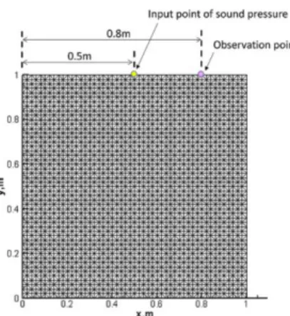
Fig. 1 shows computational model of inverse analysis. Input point of sound pressure and observation point respectively set (x, y) = (0.5m, 1.0m) and (x, y) = (0.8m, 1.0m). The flux concerned with sound pressure shown Eq.
(6) sets zero in outward boundary except for input point. Now we inverse analysis about problem to obtain sound
pressure which sound pressure in observation point approximates to the observed sound pressure in input point.
Sound pressure in input point is represented pulse signal. On the other hand, the wave size varies with hammering power, target materials and other reasons. In this case, when to do hammering test, if hammering signal can be obtained by measurement value in advance, we think the analysis is able to apply to simulation of supporting hammering test. Thus, in this study, wave of sound pressure about pulse wave shown Eq. (14) is assumed correct value on input point.
( )2
exp t R
p (14)
where R indicates pulse rise time. We set R = 50[s]. The wave given to forward analysis to be given correct sound pressure in input point is adopted artificial measurement value. In this consideration, first of all, to inverse analysis about condition is zero with time in input point. Next, iterate computation according to the flowchart shown prior chapter. Finally, considering about wave of sound pressure shown Eq. (19) is obtained by measurement value in input point. The following Tab. 1 shows computational conditions.
Figure 1: Computational model of inverse analysis Table 1 Computational conditions
Total number of nodes 2601
Total number of elements 5000
Time increment Δt, sec. 0.04
wave velocity , m/sec 0.01
Time step 10000
Diagonal values at the first iteration in Sakawa-Shindo method[3] 1.0 Sound pressure at the first iteration in input point, Pa 0.0
Convergence criterion ε 10-6
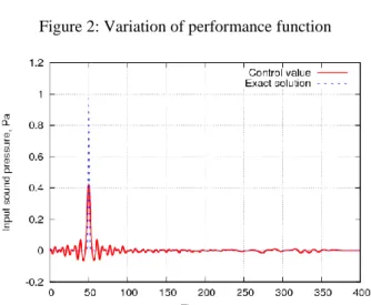
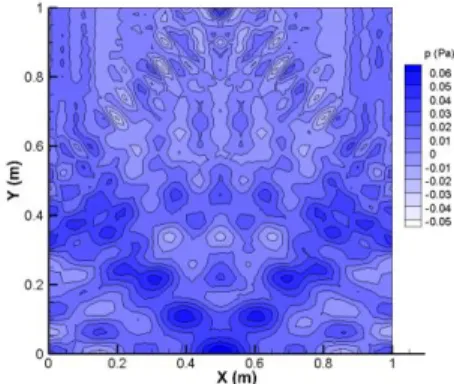
As a result of inverse analysis, performance function shown Fig. 2 is obtained. It can be seen performance function generally converges zero. In addition, Time history of sound pressure in input point and in observation point respectively shown Fig. 3 and Fig.4. Fig. 3 shows that sound pressure obtained inverse analysis observes ringing phenomena before and after pulse signal and maximum correct value of pulse is 1.0, although analysis value is about 0.42. However, pulse rise time qualitatively correspond to correct value, a value close to correct is obtained. Fig. 4 shows comparison of sound pressure at final iteration in measurement point and sound pressure of correct value. As a result, it can be seen analysis value generally corresponds to measurement value in observation point. Distributions of sound pressure when converging performance function shown Figs. 5 - 8. These show result at intervals of 100 seconds. Sound pressure given in input point is propagated. It can be seen the analysis is properly concluded.
Figure 2: Variation of performance function
Figure 3: Time history of sound pressure in input point
Figure 4: Time history of sound pressure in measurement point
Figure 5: Distribution of sound pressure at 100 sec. Figure 6: Distribution of sound pressure at 200 sec.
Figure 7: Distribution of sound pressure at 300 sec. Figure 8: Distribution of sound pressure at 400 sec.
5. Conclusions
In this study, inverse analysis for input sound pressure identification in nondestructive hammering test was carried out. The wave equation was applied to compute the propagation of sound pressure. Moreover, the finite element method was applied to discretize the wave equation in space, and the method proposed by Krenk was applied to discretize the wave equation in time. Then, the adjoint variable method was applied to identify the input signal of hammering test. As a result of numerical experiments, it was found that the input sound pressure can be appropriately identified by using the present method. In addition, as the future work of this study, it is necessary to transform the sound pressure value to the sound pressure level at the input and the output points, and to classify the type of defect size and depth based on the sound pressure level at those points.
Acknowledgements
The computations were mainly carried out using the Fujitsu PRIMAGY CX400 computer facilities at Kyushu University’s Research Institute for Information Technology. We wish to thank the staff at Kyushu University’s Research Institute for Information Technology.
References
[1] A.Nouchi, Dageki ni yoru KashinTokusei wo Kouryo shita Syuuhasuu Outou Kansu ni motoduku Konkrito Naibu no Kekkan Hyouka (Evaluation of internal defects in concrete based on frequency response function considering vibration characteristics by hitting), Proceedings of the Japan Concrete Institute, 38 (1), 2133-2138, 2016. (In Japanese)
[2] S.Krenk, Dispersion-corrected explicit integration of the wave equation, Computer Methods in Applied Mechanics and Engineering, 191, 975-987, 2001.
[3] Y.Sakawa and Y.Shindo, On Global Convergence of An Algorithm for Optimal Control, IEEE Transactions on Automatic Control, ac-25 (6), 1149-1153, 1980.