Instructions for use
A uthor(s ) NE W T ON,Paul, K ; S A K A J O,T akashi
C itation Hokkaido University Preprint S eries in Mathematics, 797: 1-19
Is s ue D ate 2006-08-01
D O I 10.14943/83947
D oc UR L http://hdl.handle.net/2115/69605
T ype bulletin (article)
sphere: IV. Ring configurations coupled to
a background field
B y Paul K. Newton and Takashi Sakajo
Department of Aerospace & Mechanical Engineering and Department of Mathematics, University of Southern California, Los Angeles, CA 90089-1191
([email protected]) and
Department of Mathematics, Hokkaido University Sapporo, Japan
We study the evolution ofN-point vortices in ring formation embedded in a back-ground flowfield that initially corresponds to solid-body rotation on a sphere. The evolution of the point vortices are tracked numerically as anembedded dynamical system along with theM contours which separate strips of constant vorticity. The full system is a discretization of the Euler equations for incompressible flow on a rotating spherical shell, hence a ‘barotropic’ model of the one-layer atmosphere. We describe how the coupling creates a mechanism by which energy is exchanged between the ring and the background, which ultimately serves to break-up the structure. When the center-of-vorticity vector associated with the ring is initially misaligned with the axis of rotation of the background field, it sets up the propa-gation of Rossby-Haurwitz waves around the sphere which move retrograde to the solid-body rotation. These waves pass energy to the ring (in the case when the solid-body field and the ring initially co-rotate), or extract energy from the ring (when the solid-body field and the ring initially counter-rotate), hence the Hamilto-nian and the center-of-vorticity vector associated with theN-point vortices are no longer conserved as they are for the one-way coupled model described in Newton & Shokraneh (2006a). In the first case, energy is transferred to the ring, the length of the center-of-vorticity vector increases, while its tip spirals in a clockwise manner towards the North Pole. The ring stays relatively intact for short times but ulti-mately breaks-up on a longer timescale. In the later case, energy is extracted from the ring, the length of the center-of-vorticity vector decreases while its tip spirals towards the North Pole and the ring loses its coherence more quickly than in the co-rotating case. The special case where the ring is initially oriented so that its center-of-vorticity vector is perpendicular to the axis of rotation is also examined as it shows how the coupling to the background field breaks this symmetry. In this case, both the length of the center-of-vorticity vector and the Hamiltonian energy of the ring achieve a local maximum at roughly the same time.
1. Introduction
We study the evolution of a ring of N-point vortices on a sphere embedded in a background flow that initially corresponds to solid-body rotation. Our main goal is to understand the nature of the coupling between the ring and the background field in order to elucidate the mechanism by which such configurations, which model the boundary between distributed coherent vortices and the backgrounds in which they are embedded, are destabilized in much more complex settings. The paper of McDonald (1999) provides an excellent discussion of many of the key effects associ-ated with geophysical vortices. We adopt a simple barotropic vorticity model on the sphere (as in DiBattista & Polvani (1998)) in order to identify several key features of the interaction process in a pristine environment where definitive statements can be made based on careful numerical experiments and comparisons with the sim-pler one-way coupled model developed in Parts I-III of this sequence (see Newton & Shokraneh (2006a), Jamaloodeen & Newton (2006), Newton & Shokraneh (2006b)). In particular, Part I in this sequence highlighted the importance of the misalignment of the center-of-vorticity vector associated with theN-point vortices with the axis of rotation associated with the solid-body velocity field. In this paper, we include the additional important physical mechanism of coupling to the background flow and the subsequent generation of Rossby waves, hence we are able to understand the combined effects of the misalignment and coupling when both act together. The strength of this approach is in our ability to isolate the key mechanisms which lead to the ring break-up and loss of integrable structure of the one-way coupled model that was established in Part I. Of course, when analyzing more complex systems such as Jupiter’s atmosphere (see Dowling (1995), Marcus (1988, 1990, 1993)), the distinction between the vorticity associated with a coherent structure (such as the Great Red Spot) and the background vorticity is far less clear.
(a) Summary of the one-way coupled model
We first summarize the one-way coupled model in order to contrast its main features with the two-way coupled model studied in this paper. In Part I of this sequence (see Newton & Shokraneh (2006a)), we introduced a model for the evolu-tion ofN-point vortices on a sphere with background solid-body rotational velocity field. The dynamical system for theN-point vortices is given by
˙ xα= 1
4π N
X
β=1
′Γ β
xβ×xα
(1−xα·xβ)+ Ωˆez×xα (α= 1, ..., N) (1.1)
xα∈R3, kxαk= 1.
The prime on the summation indicates that the singular termβ=αis omitted and initially, the vortices are located at the given positionsxα(0)∈R3, (α= 1, ..., N). The denominator in (1.1) is the chord distance between vortex Γα and Γβ since
e
zJ
!
! !
! ! ! ! ! ! ! 0
1
2
3
4
5
6
7
8
9
"
e
zJ
#
(a) (b)
$0
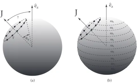
Figure 1. Initial configuration with N equal strength point vortices (Γ) evenly spaced
around a spherical cap which gives rise to the J-vector as shown. (a) The size of the
spherical cap is characterized by the base half-angleθ0, while the orientation with respect
to the axis of rotation is characterized by angleγ. (b) 10 constant vorticity strips ωn =
const. with 9 contours that require tracking. The constant valuesωn are chosen so that
they approximate the vorticity distribution corresponding to solid-body rotation around the z-axis. See text for more details.
flow, which remains in solid-body form. Hence, we called this a one-way coupled model.
The key to understanding this simplified model is the realization that thecenter of vorticityvectorJassociated with the point-vortices, defined as
J=
N
X
α=1
Γαxα= N
X
α=1 Γαxα,
N
X
α=1 Γαyα,
N
X
α=1 Γαzα
!
= (Jx, Jy, Jz), (1.2)
satisfies
˙
J= Ωˆez×J, (1.3)
as can be verified by multiplying (1.1) by Γα, summing overα, and using the fact that xα×xβ = −xβ×xα. Eqn (1.3) is solved by applying the rotation matrix, MΩ(t), to J(0)
J(t) =MΩ(t)J(0). (1.4)
MΩ(t) is given by
MΩ(t) =
cos Ωt −sin Ωt 0 sin Ωt cos Ωt 0
0 0 1
(1.5)
and is a unitary matrix with the property
MT
From this we conclude that the length ofJis constant since
kJk2=<J,J>=<MΩJ(0),MΩJ(0)>=<MT
ΩMΩJ(0),J(0)>=kJ(0)k2, (1.7)
while the components break up into two conserved quantities
Jx2+Jy2=C1= const. (1.8)
Jz=C2= const. (1.9)
The remaining important conserved quantity is the Hamiltonian,H, given by
H=− 1
4π N
X
α<β
ΓαΓβlogkxα−xβk. (1.10)
As theN-vortices evolve under their mutual interaction aroundJ, it in turn rotates with frequency Ω about the z-axis, maintaining a fixed angleγ with respect to the axis. See Part I for more details.
We made the simple observation that it is the misalignment of the center of vorticity vector with the axis of rotation (γ6= 0) that is an important ingredient in understanding the dynamics of the vortices. The key to understanding the ramifica-tions of the misalignment is to understand how the unitary operator,LJ
Ω(t), affects trajectories on the aligned (γ = 0) non-rotating (Ω = 0) sphere. The relation be-tween solutions of the original rotating system,xα(t), and solutions of the aligned non-rotating systemzα(t), is via the linear operatorLJ
Ω(t)≡MΩ(t)M−z1M−y1
xα(t) =LJ
Ω(t)zα(t). (1.11)
The matricesMy andMzserve to alignJ(0) with thez-axis, hence are defined as:
Mz=
cosγz −sinγz 0 sinγz cosγz 0
0 0 1
, (1.12)
My=
cosγy 0 sinγy
0 1 0
−sinγy 0 cosγy
. (1.13)
We note that the operatorLJ
Newton (1998, 2000), Newton & Shokraneh (2006a)) of the pureN-vortex problem on the non-rotating sphere remains largely intact in this one-way coupled model.
The goal of the current paper is to understand the effects of coupling the back-ground field to the point-vortex dynamics, with particular attention paid to the misalignment of theJvector. We will elucidate the effect of the two-way coupling to the dynamics of theN-point vortices, which are embedded in the background field and are able to exchange energy with it. The model we adopt, called a one-layer spherical barotropic model, was used in DiBattista & Polvani (1998) to understand the evolution of dipoles. What was not emphasized in that study is the role the mis-alignment plays in the overall dynamical processes. In fact, if the center of vorticity vector is initially aligned with the axis of rotation, then this effect plays no role. To set the stage for the descriptions to follow, we show in figure 1 the schematic diagram associated with the point-vortex ring and the discretized background field described in more detail later. Note the initial misalignment ofJwith the axis of rotation as characterized by settingγ6= 0 initially. As the ring and the background strips evolve (as shown in figures 2 and 3), theM−1 contours associated with the
M strips deform and wrap around the point-vortices, while the ring is destabilized and ultimately destroyed. Details of this process, with particular emphasis on the exchange of energy between the ring and the background follow in Sections 3 and 4 after a description of the numerical method.
2. The numerical method
The numerical method we use is based on that described in DiBattista & Polvani (1998). The vorticity on the unit sphere evolves according to the equation Dω
Dt = 0, where ω = x·(∇ ×u) and u is the two-dimensional velocity field. The incom-pressibility condition∇ ·u= 0 implies the existence of streamfunctionψ(x), where u=x× ∇ψ, which gives rise to the relation ω= ∆ψ. Inversion of this expression gives rise to
ψ(x) =
Z Z
S
G(x,x′)ω(x)dA (2.1)
whereG(x,x′) is the Green’s function on the sphereG(x,x′) = −1
4πlog|x−x′|
2.
As in Bogomolov (1978), we think of the vorticity field as being made up of two parts,ω(θ, φ) =ωN+ωSB.ωN is the vorticity due to theN-point vortices, i.e.
ωN = 1 sinθ
N
X
α=1
Γαδ(θ−θα, φ−φα), (2.2)
where (θα, φα) represents the position of theαth point vortex in spherical coordi-nates. This gives rise to the velocity field
uv(x) = Γ 4π
N
X
α=1
xα×x
1−x·xα. (2.3)
T:0.00
T:1.00
T:2.00
T:3.00
T:4.00
T:4.50
T:5.00
T:5.50
T:6.00
T:6.50
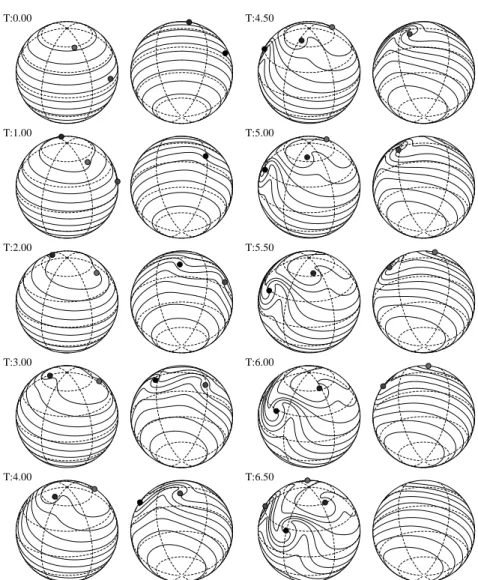
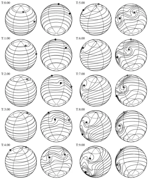
Figure 2. Evolution of ring configuration and contours withN= 4 andM = 10 and
frequency ratio 4:1. Orientationγ=π/4 andθ0=π/4.T = 0.0−6.5 in dimensionless
units.
z = cosθ0, then they are rotated around thex-axis by the angle γ. The strength of each vortex point Γ is determined so that the frequency ratio between the ring’s rotation frequency and the solid-body frequency becomesm:n. Namely,
ω: Ω = Γ(N−1) cosθ0 4πsin2θ0
: 1
2 =m:n. (2.4)
T:8.00
T:8.50
T:9.00
T:9.50
T:10.00
T:10.50
T:11.00
T:11.50
T:12.00
T:12.50
Figure 3. Same as previous figure but withT = 8.0−12.5 in dimensionless units. Note
the wrapping of the contours around the point vortices effectively increases their strength with respect to the background. The ring stays relatively intact throughout the evolution.
represent the M contour curves, in which 0 ≤ θ < 2π is a parameter along the contour curve andtis time. The initial position of Xαis given by
Xα(θ,0) =p1−z2
αcosθ,
p
1−z2
αsinθ, zα
, α= 1, . . . , M, (2.5)
where
zα= 1− 2α
M + 1. (2.6)
piecewise constant, and the jump across the contour curveXα, say ˜ωα, is given by
˜
ωα= 1
2(zα−1−zα+1), (2.7) in which z0 = 1 and zM+1 =−1. The velocity field induced by the M + 1 zonal vorticity strips is represented by the boundary integral along theM contours (see Dritschel (1989), Dritschel & Polvani (1992), Polvani & Dritschel (1993) for further relevant discussions)
us(x) =−
M
X
α=1
ωα
Z 2π
0
log|x−Xα|2 ∂Xα
∂θ dθ. (2.8)
The numerical computation becomes unstable when the vortex points approach very close to the contour curves. Thus, the interaction between the vortex points and the vorticity strips is evaluated by a velocity field regularized by the vortex blob method. Introducing a smallδ >0, the regularized velocity fields are given by
u(δ)
v (x) = Γ 4π
N
X
α=1
xα×x
1 +δ2−x·xα, (2.9)
u(δ)
s (x) = − M
X
α=1
ωα
Z 2π
0
log |x−Xα|2+δ2 ∂Xα
∂θ dθ. (2.10)
The regularization parameterδ was successfully introduced to compute the long-time evolution of a vortex sheet (Krasny (1986)) and is described thoroughly in the book of Cottet and Koumoutsakos (2000). In our case, the regularization stabilizes the numerical computation and makes it possible to track the evolution of the vortex points and contours without using the contour surgery technique (Dritschel (1989)).
Accordingly, the equations we consider are
∂xj
∂t = u
′
v(xj) +us(δ)(xj), j= 1, . . . , N, (2.11)
∂Xk
∂t = us(Xk) +u
(δ)
v (Xk), k= 1, . . . , M, (2.12)
where u′
v equals to the summation terms in (1.1). The boundary integral along each of the contours is approximated by the trapezoidal rule with 4096 points. The temporal integration of (2.11) and (2.12) are carried out with the fourth order Runge-Kutta method, for which the time step size is ∆t= 0.01. The regularization parameter is fixedδ= 0.1. We have done numerical computations for various values ofδ, and confirmed that the qualitative numerical results are relatively insensitive to changes inδ.
3. Rings
(a) Two-way coupled ring dynamics: co-rotation
two_way one_way
N
(a)
(b)
(c)
N
(d)
Time Time
0 2 4 6 8 10 12
1.04 1.06 1.08 1.1 1.12
L
eng
th o
f J v
ec
to
r
E
ner
g
y
o
f ring
0 2 4 6 8 10 12 14
0.03 0.034 0.038 0.042
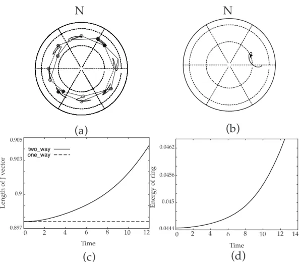
Figure 4. (a) Evolution of point vortices in a frame of reference rotating with the back-ground frequency of the one-way coupled model with a frequency ratio 4:1. Note that the ring briefly reverses direction, but as the strength of the vortices increases, it regains it original rotational direction and the ring remains relatively intact. (b) Evolution of the tip
of the center of vorticity vectorJassociated with the ring. Note that it rotates up towards
the North Pole. (c) Evolution of the length of the center of vorticity vectorkJkwhich is
constant in the one-way coupled model but not when the ring is coupled to the back-ground flow. In this case, as the vortices increase their strength by wrapping themselves
in the contours, the length of J increases. (d) The Hamiltonian is no longer conserved
when the ring is coupled to the background. In this case, since the ring is co-rotating with the background, it is gaining energy from it.
dynam-T:0.00
T:1.00
T:2.00
T:3.00
T:4.00
T:5.00
T:5.50
T:6.00
T:6.50
T:7.00
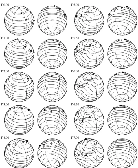
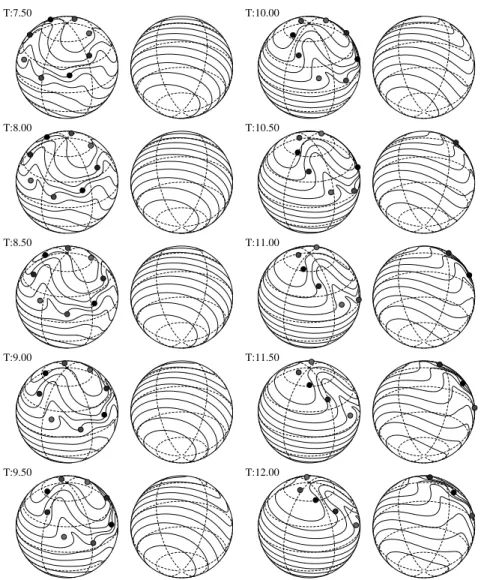
Figure 5. Evolution of ring configuration and contours withN= 8 andM = 10 and
frequency ratio 4:1. Orientationγ=π/4 andθ0=π/4.T = 0.0−7.0 in dimensionless
units.
ical evolution of the system, our goal is to extract the main features of the effect of the misalignmentγ 6= 0 during the interaction process. In Part I, figures 11-14 show the evolution of a ring in the one-way coupled model for the caseN = 4, with orientation anglesγ=π/4, π/2,3π/4 and frequency ratiosω: Ω = 1 : 1; 2 : 1; 3 : 1. The trajectories of the vortices in this model move on closed periodic orbits in all cases. Note that for the caseγ=π/4, the ring co-rotates with the solid-body field, while for the caseγ= 3π/4 it counter-rotates. The caseγ=π/2 is a special sym-metric orientation which we will describe later. The length of the center-of-vorticity vector associated with the ring is constant, as is the Hamiltonian energy.
well-T:7.50
T:8.00
T:8.50
T:9.00
T:9.50
T:10.00
T:10.50
T:11.00
T:11.50
T:12.00
Figure 6. Same as previous figure but withT = 7.5−12.0 in dimensionless units. Note
the wrapping of the contours around the point vortices effectively increases their strength. The ring stays relatively intact throughout the evolution.
known fact (also seen nicely in by DiBattista & Polvani (1998)) that in the absence of point vortices, the contours support the propagation (see their figure 4) of Rossby-Haurwitz waves which moveretrogradewith respect to the solid-body rotation. The general processes by which Rossby-Haurwitz waves propagate and lose stability are by now quite well documented (see, for example Craig (1945), Silberman (1954), Lorenz (1972), Hoskins (1973), Gill (1974), Baines (1976), Pedlosky (1987)). The mechanisms by which their coupling to structures embedded in the flow serve to break-up these structures is far less understood.
Consider the sequence of simulations shown in figures 2, 3 for the caseN = 4,
north pole north pole north pole north pole north pole north pole north pole north pole north pole north pole north pole north pole north pole north pole north pole north pole north pole north pole north pole north pole north pole north pole north pole north pole north pole north pole north pole north pole north pole north pole north pole north pole north pole north pole north pole north pole north pole north pole north pole north pole north pole north pole north pole north pole north pole north pole north pole north pole north pole north pole north pole north pole north pole north pole north pole north pole north pole north pole north pole north pole north pole north pole north pole north pole north pole north pole north pole north pole north pole north pole north pole north pole north pole north pole north pole north pole north pole north pole north pole north pole north pole north pole north pole north pole north pole north pole north pole north pole north pole north pole north pole north pole north pole north pole north pole north pole north pole north pole north pole north pole north pole north pole north pole north pole north pole north pole north pole north pole north pole north pole north pole north pole north pole north pole north pole north pole north pole north pole north pole north pole north pole north pole two_way one_way
N
N
(a)
(b)
(c)
(d)
L eng th of J vec
to r E ner g y o f ring Time Time
0 2 4 6 8 10 12 0.04440 2 4 6 8 10 12 14
0.045 0.0456 0.0462 0.897 0.9 0.903 0.905
Figure 7. Same parameters as figure 4 but withN = 8. The conclusions are robust with
respect to changes inN.
Pole. It’s length increases (see figure 4(c)) and the Hamiltonian energy associated with the ring (shown in figure 4(d)) gains energy from the background. This general sequence of events is quite robust to changes in the number of point vortices making up the ring, as shown in the sequence of figures 5, 6 and figure 7 forN = 8.
(b) Two-way coupled ring dynamics: counter-rotation
T:0.00
T:1.00
T:2.00
T:3.00
T:4.00
T:5.00
T:6.00
T:7.00
T:8.00
T:9.00
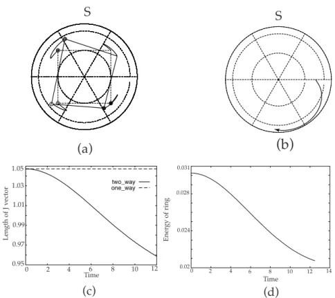
Figure 8. Evolution of ring configuration and contours withN = 4 andM = 10 and
fre-quency ratio -4:1. Orientationγ=π/4 andθ0=π/4.T = 0.0−9.0 in dimensionless units.
In contrast to the co-rotating case, the wrapping of the contours around the point vortices
south pole south pole south pole south pole south pole south pole south pole south pole south pole south pole south pole south pole south pole south pole south pole south pole south pole south pole south pole south pole south pole south pole south pole south pole south pole south pole south pole south pole south pole south pole south pole south pole south pole south pole south pole south pole south pole south pole south pole south pole south pole south pole south pole south pole south pole south pole south pole south pole south pole south pole south pole south pole south pole south pole south pole south pole south pole south pole south pole south pole south pole south pole south pole south pole south pole south pole south pole south pole south pole south pole south pole south pole south pole south pole south pole south pole south pole south pole south pole south pole south pole south pole south pole south pole south pole south pole south pole south pole south pole south pole south pole south pole south pole south pole south pole south pole south pole south pole south pole south pole south pole south pole south pole south pole south pole south pole south pole south pole south pole south pole south pole south pole south pole south pole south pole south pole south pole south pole south pole south pole south pole south pole south pole south pole two_way one_way
(a)
S
(b)
(c)
(d)
S
Time Time L eng th of J vec
to r E ner g y o f ring
0 2 4 6 8 10 12
0.95 0.97 0.99 1.01 1.03 1.05
0 2 4 6 8 10 12 14 0.02
0.024 0.028 0.031
Figure 9. (a) Evolution of point vortices in a frame of reference rotating with the back-ground frequency of the one-way coupled model with a frequency ratio -4:1. In contrast to figure 4, the original rotational direction of the ring is never regained and the ring loses its coherence much more quickly. (b) Evolution of the tip of the center of vorticity vector
J associated with the ring. Note that it still rotates towards the North Pole. (c)
Evolu-tion of the length of the center of vorticity vector kJk which decreases as the contours
wrap around the vortex centers. (d) The Hamiltonian is no longer conserved when the ring is coupled to the background. In this case, since the ring is counter-rotating with the background, it is losing energy to it.
A case where the ring initially counter-rotates with respect to its background is shown in figures 8 and should be contrasted with the previous sequence of figures. The parameters for this case are the same as those in figures 2, but the frequency ratio is now -4:1. As the contours wrap around the point vortices, their effective strengthdecreases(in absolute magnitude), causing the ring to diminish in strength relative to the background. Because of this, it never regains its original rotational direction, as shown in figure 9(a) which should be contrasted with the corresponding figure 4(a). In addition, the ring loses its coherence more quickly than the co-rotating case, the tip of the Jvector spins towards the North Pole and decreases its effective length while losing energy to the background.
background field, the instability does not develop as quickly, nor is it as violent as is the case when the ring counter-rotates with respect to the background.
T:0.00
T:1.00
T:2.00
T:3.00
T:4.00
T:5.00
T:6.00
T:6.50
T:7.00
T:7.50
Figure 10. Evolution of ring configuration and contours withN = 4 andM = 10 and
frequency ratio 2:1. Orientationγ =π/2 and θ0 =π/4.T = 0.0−7.5 in dimensionless
units. Note that for this orientation, if the sign of Γ is reversed, the evolution of the system will be identical but in the opposite hemisphere.
(c) γ=π/2: Breaking symmetry
T:8.00
T:8.50
T:9.00
T:9.50
T:10.00
Figure 11. Same as previous figure but withT = 8.0−10.0 in dimensionless units. Note
the wrapping of the contours around the point vortices effectively increases their strength. The ring stays relatively intact throughout the evolution.
This case in the one-way coupled model, where theJvector remains perpendicular to the axis of rotation, is shown in figure 13 of Part I (Newton & Shokraneh (2006a)). For the two-way coupled case, the evolution sequence is shown in figures 10 and 11. For this orientation, the ring initially cuts the contours perpendicularly and there is no distinction between co-rotation and counter-rotation. In the one-way coupled model, J would remain perpendicular to the axis of rotation throughout the entire evolution, as there is no mechanism by which this symmetry is broken. In this case, however, the coupling to the background provides such a symmetry-breaking mechanism. As the vortices within the ring wrap the contours around themselves, the perfect ring structure and its orientation are destroyed immediately. The shape of the ring, the evolution of the tip ofJ, its length, and the evolution of
north pole north pole north pole north pole north pole north pole north pole north pole north pole north pole north pole north pole north pole north pole north pole north pole north pole north pole north pole north pole north pole north pole north pole north pole north pole north pole north pole north pole north pole north pole north pole north pole north pole north pole north pole north pole north pole north pole north pole north pole north pole north pole north pole north pole north pole north pole north pole north pole north pole north pole north pole north pole north pole north pole north pole north pole north pole north pole north pole north pole north pole north pole north pole north pole north pole north pole north pole north pole north pole north pole north pole north pole north pole north pole north pole north pole north pole north pole north pole north pole north pole north pole north pole north pole north pole north pole north pole north pole north pole north pole north pole north pole north pole north pole north pole north pole north pole north pole north pole north pole north pole north pole north pole north pole north pole north pole north pole two_way one_way
N
N
(a)
(b)
(c)
(d)
L eng th of J vec
to
r
0 2 4 6 8 10
Time 2.088 2.092 2.096 2.1 2.104 E ner g y o f t he ring Time 10 8 6 4 2 0 0.1205 0.122 0.1235 0.125
Figure 12. (a) Evolution of point vortices in a frame of reference rotating with the
back-ground frequency of the one-way coupled model with a frequency ratio 2:1 andγ=π/2.
For this symmetric case, the ring briefly reverses direction, but as the strength of the vortices increases, it regains it original rotational direction as in the previously discussed
co-rotating cases. (b) Evolution of the tip of the center of vorticity vectorJ associated
with the ring. Note that it spirals up towards the North Pole. (c) Evolution of the length
of the center of vorticity vectorkJkwhich is constant in the one-way coupled model but
not when the ring is coupled to the background flow. In this case, as the vortices increase
their strength by wrapping themselves in the contours, the length ofJevolves in a more
complex manner that either the co-rotating or counter-rotating cases discussed previously. Initially it’s length increases but the reverses direction. (d)Evolution of the Hamiltonian
energy of the ring which achieves a local maximum at roughly the same time askJk.
4. Discussion
• The ring triggers an instability in the background field setting up Rossby-Haurwitz waves which travel along the contours moving retrograde to the solid-body rotation direction;
• These waves cause the ring to alter its rotational direction;
• The contours wrap around the point-vortices, increasing their effective strength in the case where the ring co-rotates with the background, decreasing it (in absolute magnitude) in the case when it counter-rotates;
• The increase in strength in the co-rotating case allows the ring to overcome the effects of the Rossby-Haurwitz waves and reverse direction again, regaining its original rotational direction;
• In the counter-rotating case, since the ring strength is effectively decreasing, the ring never regains its original rotational direction;
• Energy is continually exchanged between the ring and the background field (i.e.H andkJkare no longer conserved) via this process of contour wrapping and the stability and integrity of the ring is compromised;
• In the special symmetric configuration whenJis initially perpendicular to the axis of rotation of the background field, the coupling provides a symmetry-breaking mechanism not present in the one-way coupled model. The evolution ofkJkandH are non-monotonic, both reaching a local maximum at roughly the same time.
A key feature of the one-way coupled model discussed in Part I was that the integrability of the non-rotating problem (Ω = 0) and the rotating problem (Ω6= 0) were identical. With the two-way coupled model, on the short timescale, the coupling to the background offers a mechanism by which the ring is destabilized and loses its coherence. On a longer timescale, since all of the main conserved quantities (JandH) are broken, it offers a natural mechanism by which integrability is destroyed and we expect that the long-time evolution of the vortices will be chaotic. Of course tracking them accurately for long enough timescales to compute quantities such as Lyapunov exponents is far more challenging than in the one-way coupled case. This is primarily because of the aggressive growth and wrapping of the many contours that must be tracked. In a simpler setting, the growth of these types of interfaces and their connection with the mixing and transport of passive particles has been studied in Newton & Ross (2006) for a perturbed point-vortex ring on the sphere without rotation. In the two-way coupled problem it is the coupling to the background that causes the ring perturbation. This, in turn, generates the Rossby waves which we identify as the main physical mechanism responsible for breakdown of the integrability and loss of coherence of the ring.
References
Baines P.G. 1976 The stability of planetary waves on a sphere, J. Fluid Mech.Vol. 73,
193–213.
Bogomolov V.A. 1979 Two dimensional fluid dynamics on a sphere.Izv. Atmos. Oc. Phys.
15(1), 18–22.
Bogomolov V.A. 1985 On the motion of a vortex on a rotating sphere.Izv. Atmos. Oc.
Phys.21(4), 298–302.
Cabral H.E., K.R. Meyer, D.S. Schmidt. 2003 Stability and bifurcations for the N+1
vortex problem on the sphere.Regular and Chaotic Dynamics,8(3), 259–282.
Cottet, G-H., P.D. Koumoutsakos 2000Vortex Methods: Theory and Practice
Cam-bridge Press, CamCam-bridge UK.
Craig R.A. 1945 A solution of the non-linear vorticity equation for atmospheric motion. J. Met.Vol. 2, 175.
DiBattista M.T., L.M. Polvani 1998 Barotropic vortex pairs on a rotating sphere.Journal
of Fluid Mechanics358, 107–133.
Dowling T.E. 1995 Dynamics of Julian atmosphere,Ann. Rev. Fluid Mech.27293–334.
Dritschel, D.G. 1989 Contour dynamics and contour surgery: numerical algorithms for extended high resolution numerical modeling of vortex dynamics in two-dimensional,
inviscid, incompressible flows,Comp. Phys. Rep.1077–146.
Dritschel D.G., L.M. Polvani 1992 The roll-up of vorticity strips on the surface of a sphere. J. Fluid Mech.Vol. 23447–69.
Gill A.E. 1974 The stability of planetary waves.Geo. Fluid. Dyn.Vol. 629.
Hoskins B.J. 1973 Stability of the Rossby-Haurwitz wave.Quart. J. Roy. Met. Soc.Vol.
99723.
Jamaloodeen M.I., P.K. Newton 2006 The N-vortex problem on a rotating sphere: II.
Heterogeneous Platonic solid equilibria.in press,Proc. Roy. Soc. London Ser. A.
Kidambi R., P.K. Newton 1998 Motion of three point vortices on a sphere. Physica D
116143–175.
Kidambi R., P.K. Newton 2000 Streamline topologies for integrable vortex motion on a
sphere.Physica D 14095–125.
Kransy R. 1986 Desingularization of periodic vortex sheet roll-up. J. Comp. Phys. 65
292–313.
Lorenz E. 1972 Barotropic instability of Rossby wave motion.J. Atmos. Sci.Vol. 29, 258.
Majda, A. 2003Introduction to PDEs and Waves for the Atmosphere and Ocean,
Courant Institute Lecture Notes, Vol. 9, American Mathematical Society, Providence RI.
Marcus, P.S. 1988 Numerical simulations of Jupiters Great Red Spot.Nature Vol. 331,
693–393.
Marcus, P.S. 1990 Vortex dynamics in a zonal shearing flow.J. Fluid Mech.215, 393-430.
Marcus, P.S. 1993 Jupiter’s Great Red Spot and other vortices.Ann. Rev. Astron.
Astro-phys.Vol. 31, 523-573.
McDonald N.R. (1999) The motion of geophysical vortices,Phil. Trans. R. Soc. Lond. A
3573427–3444.
Newton P.K. 2001The N-Vortex Problem: Analytical Techniques. Applied Math.
Sci.145, Springer-Verlag, New York.
Newton P.K., H. Shokraneh. 2006 The N-vortex problem on a rotating sphere: I.
Multi-frequency configurations.Proc. Roy. Soc. London Ser. AVol. 462, 2065, 149–169.
Newton P.K., H. Shokraneh. 2006 The N-vortex problem on a rotating sphere: III. Dipoles as interacting billiards, USC preprint.
Newton P.K., S.D. Ross 2006 The restricted four vortex problem,in press,Physica D.
Pedlosky J. 1987Geophysical Fluid Dynamics2nd Ed. Springer-Verlag, New York.
Polvani L.M., D.G. Dritschel. 1993 Wave and vortex dynamics on the surface of a sphere. J. Fluid Mech.255, 35–64.