カーネル平滑化統計量に基づくノンパラメトリック推測

(1)

九州大学学術情報リポジトリ

Kyushu University Institutional Repository

カーネル平滑化統計量に基づくノンパラメトリック推測

森山, 卓

https://doi.org/10.15017/1931731

出版情報：Kyushu University, 2017, 博士（数理学）, 課程博士バージョン：

権利関係：

(2)

Nonparametric inference based on kernel smoothed statistics

Doctoral dissertation

Taku MORIYAMA

Graduate School of Mathematics, Kyushu University 744 Motooka, Nishi-ku, Fukuoka 819-0395, Japan

February 14, 2018

(3)

Abstract

We consider nonparametric inference based on ‘kernel smoothed’ statistics. Nonparamet- ric methods can handle data from unspecified distributions, which is called as ‘robust’ to model assumptions. An empirical distribution function estimator and a histogram density estimator are known as classical estimators, but they are not continuous as functions of observed values.

Kernel type nonparametric estimators have their origin in Rosenblatt (1956) who obtained a (one-dimensional) kernel type density estimator by smoothing the histogram density estimator. The kernel smoothing method has been widely applied, and various smoothed nonparametric statistics were proposed. However, some problems which kernel type statistics own are reported. Their asymptotic convergence rates depend on smoothing parameters.

In addition, optimal convergence rates of most kernel type estimators are (uniformly) slower than that of ‘parametric’ estimators in general settings.

We first focus on kernel type estimation of a hazard ratio function and then discuss reduction of an asymptotic mean squared error of kernel hazard ratio estimators. The hazard ratio is a fundamental measure in survival analysis and risk management. We obtain a new kernel hazard ratio estimator by modifying ´Cwik and Mielniczuk (1989)’s method, and its asymptotic properties are examined. The proposed method gives precise estimation especially in exponential or gamma cases, which play a central role in survival analysis.

Next, we discuss the so-called ‘boundary bias problem’ in naive kernel density estimation introduced by Rosenblatt (1956). In naive kernel estimation of a probability density, it is implicitly assumed that the support of the density function covers the whole real line. If the assumption does not hold, the kernel density estimator possibly has a boundary bias.

Therefore, we should also take care with an unexpected boundary bias when the ‘exact’

support is unknown.

As the second theme of this thesis, we study the boundary bias problem in such case.

We propose a new method for simultaneous nonparametric estimation of the probability density and its support. The proposed method detects the boundary and returns a modified density estimator which is free from the unexpected boundary bias. Moreover, we discuss an extension to a simple multivariate case and propose a new method for estimating joint probability density functions.

Lastly, we consider application of the kernel smoothing method to statistical hypothesis testing. For the one sample location problem, the sign and Wilcoxon’s signed rank tests are distribution-free, but the two tests have a problem with their p-values because of their discreteness. We confirm the problem and propose two tests which are obtained by smoothing the discrete test statistics. The proposed tests can solve the problem of thep-values, and we derive asymptotic properties of the smoothed tests. The smoothed tests are equivalent to

(4)

the discrete ones in the sense of Pitman’s asymptotic eﬃcacy respectively, and the proposed tests are higher-order asymptotically robust to model assumptions (that is, distribution-free) if the kernel functions and smoothing parameters are suitably selected. Thus, the smoothed tests inherit good properties of the original tests.

Moreover, for the two sample case, we show that the median and Wilcoxon’s rank sum tests have the same problem with their p-values. The median and Wilcoxon’s rank sum tests can be seen as two-sample versions of the sign and Wilcoxon’s signed rank tests respectively, and we propose smoothed tests which solve the problem in a similar manner. We obtain local asymptotic powers of the proposed tests and examine approximations of their p-values.

(5)

Acknowledgement

I would like to express my sincere gratitude to my supervisor Professor Yoshihiko Maesono for his guidance, valuable suggestions and kind support for my research.

I am grateful to Professor Ryuei Nishii, Professor Hiroki Masuda, Professor Yoshiyuki Ninomiya, and Professor Kei Hirose for their valuable comments which helped me to improve my research.

I would like to thank my friends for daily discussions. We have discussed a lot of interests, which encouraged me.

Finally, I want to thank my family for supporting me throughout all my studies at Kyushu University.

Taku Moriyama February 14, 2018

(6)

1 Introduction

In traditional statistical inference, ‘parametric’ methods have been widely used in our deci- sion making. Parametric methods infer a finite number of parameters (e.g. the mean and variance) which index specified statistical structures. Now, we consider to infer a function p (e.g. probability density, hazard ratio, conditional density, regression function etc.) from data. Though a functional space P, which includes p, is infinite dimensional, the obtained sample size is always finite. Therefore, it seems to be natural to restrict the space P to a finite dimensional one Pθ ={p_θ|θ ∈ Θ} (called parametric family) indexed by a parameter θ. Then, we do statistical inference for the parameter θ which is of our interest (parametric method). In estimation of an underlying density function, we usually assume that the probability density belongs to a family of specified distributions (e.g. normal distributions).

Exponential family are known as a wide class and used to describe various random behaviors.

Parametric estimators (e.g. maximum likelihood estimator) may be ‘√

n-consistent’, which is usually an optimum rate in general settings. In statistical testing for a underlying structure, not ‘approximate’ (or ‘asymptotic’) but ‘exact’ p-values of parametric test statistics may available, by specifying the structure under the null hypothesis. That is why parametric methods have gotten both researchers’ and practitioners’ attentions.

However, in both statistical estimation and testing, parametric methods work well if and only if the true function p belongs to the parametrized family Pθ. This means that the parametric function estimator p_b_θ, which is obtained by replacing θ with an estimated θ,b never converge to pin an ordinary sense whenp /∈Pθ. ‘Nonparametric’ methods restrict P to not finite but ‘infinite’ dimensional spaces. In other words, we do not make any restrictive assumptions about the class of the true function p. In hypothesis testing, this is often called as being ‘robust’ to model assumptions or ‘distribution-free’. The good property is needed to control ‘type I error’ especially when parametric classes of the underlying distribution cannot be specified.

Let X₁,· · · , X_n be independently and identically distributed (i.i.d.) random variables with a distribution function F and f denotes the corresponding probability density function.

Unless stated, all observed values are scalar, and the support of each probability density function covers the whole real line (that is,supp(f) = R). Traditionally, an empirical distribution function estimatorF_nis well-known as a nonparametric estimator of the distribution function F. Random phenomena are described uniquely by their probability distribution functions, and so estimation of the distribution functions gives us much information. For example, a population mean defined by E[X] = ∫

xf(x)dx can be estimated by E[X] =[ ∫

xdF_n(x), where the integral is a Riemann-Stieltjes integral. In fact, E[X] coincides with a sample[ mean ¯X =n⁻¹∑n

i=1X_i. The assumption which ensures the asymptotic convergence of F_n is much weak (see Yamato (1973)), however, the estimated distribution function is not continuous. In addition, we cannot obtain any smooth density estimators by diﬀerentiating F_n. A

(8)

histogram estimator is known as a conventional density estimator given by f_n(x) = 1

mn

∑n i=1

∑

j∈Z

I(x∈L_j)I(X_i ∈L_j),

where I is the indicator function I(A) = 1 (if A occurs), = 0 (if A fails). L_j = [a₀ + (j − 1)m, a₀+jm) anda₀ is a selected origin. However, the density estimatorf_nis not continuous.

By smoothing the histogram estimator, Rosenblatt (1956) obtained a smooth nonparametric estimator of the probability density function f. This is called as kernel density estimator and given by

f(x) =b

∫ k

(x−y h

)

dF_n(y),

wherekis a probability density function and called as kernel function. The smoothing parameter h is called as bandwidth and satisfies bothh→0 andnh→ ∞(asn → ∞). Properties of the kernel density estimator have been investigated well, and Tsybakov (2009) gives a good introduction of them. A smooth kernel estimator Fb of the cumulative distribution function was derived by smoothing the empirical distribution function F_n, and the kernel smoothing method has been widely applied to traditional discrete nonparametric statistics.

Although various kernel smoothed statistics are proposed, most of them are not √ n- consistent. For example, an optimal asymptotic convergence rate of the kernel density estimator fbis of order n⁻^2/5. In Chapter 2, we discuss improvement of a naive kernel estimator of a hazard ratio in the sense of a mean squared error (M SE). The hazard ratio function is a fundamental measure of the diﬀerence between several risk groups and given by

H(x) = f(x) 1−F(x).

By replacing F andf with the kernel estimatorsFb andfbrespectively, the naive kernel type estimator He was obtained. The optimal asymptotic convergence rate of the naive estimator is generally dominated by the numerator fb and coincides with that of fb. By modifying Cwik and Mielniczuk (1989)’s method, we obtain a new kernel hazard ratio estimator´ Hb and examine its asymptotic properties. Moreover, we compare the proposed estimatorHb with He in the sense of an asymptotic mean squared error (AM SE). Indeed, the optimal convergence rate of AM SE ofHb is not diﬀerent from that of the naive estimatorH. However, it is showne that Hb performs asymptotically better, especially in exponential or gamma cases, which are important in survival analysis.

In Chapter 3, we focus on the so-called ‘boundary bias’ problem in naive kernel density estimation introduced by Rosenblatt (1956). To ensure the consistency of the density estimator fb, in fact, it is implicitly assumed that the support of the underlying probability density covers the whole real line (that is, supp(f) = R). When the obtained sample are

(9)

(d-dimensional) multivariate, it is supposed that the support covers the whole space (R^d).

However, when the assumption does not hold, the kernel density estimator fbpossibly loses its consistency near the boundary of the support, on account of a boundary bias of order 1 (boundary bias problem). If we know the support ‘exactly’, we may reduce the bias by applying boundary bias reduction methods.

When the support is unknown, the kernel density estimatorfbpossibly has an unexpected boundary bias. We insist on the necessity of estimating the support and propose a new method for nonparametric density estimation which is free from the unexpected boundary bias in such case. The proposed method detects the boundary and gives a modified density estimator simultaneously. As mentioned by Hall and Park (2002), it is natural to estimate the support by the sample maximum (and minimum) and modify the naive kernel density estimator. However, it is shown that the proposed method gives numerically precise density estimation in the boundary region when the support is unknown. Moreover, we discuss an extension to a simple multivariate case and propose a new method for estimating joint probability density functions. By utilizing nonparametric copula estimators, the proposed method combines marginal densities, which are estimated by the proposed single variable method (in one-dimensional cases), and then returns a modified joint probability density estimator. It is shown that the obtained density estimator is also free from an unexpected boundary bias when the support of the underlying joint density cannot be specified.

In Chapter 4, we consider application of the kernel smoothing method to (discrete) distribution-free test statistics and focus on the sign and Wilcoxon’s signed rank tests in the one-sample location problem. As pointed out by Lehmann and D’abrera (2006) and Brown et al. (2001), p-values of the sign test statistic may make a big jump in response to a change in data values especially when the obtained sample size is small. Because of this, p-values of the sign test are frequently larger than those of the Wilcoxon’s test, and so the discrete tests may allow us to make an arbitrary choice of the two tests.

We first confirm this problem of the p-values and then propose new smoothed sign and Wilcoxon’s signed rank tests. The original sign S and Wilcoxon’s signed rank test statistics W are equivalent to estimators of the probabilities P[X₁ >0] andP[^X¹^+X₂ ² >0] respectively, and the smoothed test statistics Se and fW are equivalent to kernel type estimators of each probabilities. We show that the smoothed tests can solve the problem of the p-values and examine asymptotic properties of the smoothed tests. The smoothed sign and Wilcoxon’s signed rank tests are equivalent to the discrete two in the sense of Pitman’s asymptotic ef- ficacy, respectively. In addition, it is shown that each diﬀerence between the standardized S and S, ande W and Wf converges to zero in L²-norm, respectively. We also discuss approximations of their p-values. To derive higher-order approximations of the p-values of the smoothed tests, Edgeworth expansions are obtained. Under some conditions, the Edgeworth expansions are free of the underlying distribution, that is, the smoothed tests are higher-order asymptotically distribution-free.

(10)

In the last Chapter, we consider application of the kernel smoothing method to the median and Wilcoxon’s rank sum tests in the two-sample location problem, in a similar manner as Chapter 4. The median and Wilcoxon’s test statistics can be seen as equivalent to estimators of the probabilitiesP[Y₁−z₀ >0] and P[Y₁−X₂ >0] respectively, where z₀ is the median of the underlying distribution of X₂. The test statistics can also be seen as two-sample versions of the sign and Wilcoxon’s signed rank tests, and we show that the median and Wilcoxon’s rank sum tests have the same problem with theirp-values. We propose smoothed tests, which inherit good properties of the original tests, and then show that the smoothed tests can solve the problem of thep-values. In addition, approximations of the smoothed tests’p-values and their local asymptotic powers are examined.

(11)

2 Kernel hazard ratio estimators and numerical com- parison

2.1 Introduction

Rosenblatt (1956) proposed a kernel estimator of the probability density function f. Many researchers have since developed various kernel estimators for distributions, regression, hazard functions, etc. Most of the kernel estimators are biased, and many researchers have studied methods of reducing the bias. These methods are based on higher order kernels, transformations of estimators, etc. Although there are many bias reduction methods, variance reduction is quite difficult. To estimate the density ratio, Ćwik and Mielniczuk (1989) proposed a kernel estimator that they called ‘direct’. The asymptotic mean squared error (AM SE) of the direct estimator is different from the AM SE of the naive estimator. In this Chapter, we devise a ‘direct’ estimator of the hazard ratio by modifying Ćwik and Mielniczuk (1989)’s method, and discuss its AM SE.

First, we will describe the direct estimator of the density ratio proposed by ´Cwik and Mielniczuk (1989). Let X₁, X₂,· · · , X_n be independently and identically distributed (i.i.d.) random variables with a distribution functionF, andY₁, Y₂,· · · , Y_nbei.i.d.random variables with a distribution functionG. f andg are the density functions ofF and G, and we assume that g(x₀)̸= 0 (x₀ ∈R). A naive estimator of the density ratio f(x₀)/g(x₀) at the point x₀ is given by fb(x₀)/bg(x₀) where

fb(x₀) = 1 h

∫ _∞

−∞

k

(x₀−w h

)

dF_n(w) and

b

g(x₀) = 1 h

∫ _∞

−∞

k

(x₀−z h

)

dG_n(z).

k is a kernel function,h is a bandwidth that satisfies h→0 and nh→ ∞ (n→ ∞), and F_n and Gn are the empirical distribution functions of X1,· · ·, Xn and Y1,· · · , Yn, respectively.

We call f(xb ₀)/bg(x₀) an ‘indirect’ estimator. ´Cwik and Mielniczuk (1989) proposed a direct estimator, given by

bf

g(x₀) = 1 h

∫ _∞

−∞

k

(G_n(x₀)−G_n(w) h

)

dF_n(w).

Chen et al. (2009) obtained an explicit form of its AM SE.

In this chapter, we develop a new ‘direct’ estimator of the hazard ratio function by modifying ´Cwik and Mielniczuk (1989)’s method and investigate itsAM SE (in Section 2.2).

We compare the naive and direct kernel estimators (in Section 2.3) and find that our direct estimator performs asymptotically better especially in exponential or gamma cases, which play a central role in survival analysis. Although the bias term of the direct estimator is

(12)

large in some cases, the asymptotic variance is always small when we use same bandwidth parameters. Proofs of the theorems herein are given in Section 2.4.

2.2 Kernel type hazard ratio estimators and asymptotic properties

The hazard ratio function is a type of relative risk and is defined as H(x₀) = f(x₀)

1−F(x0).

The meaning of H(x)dx is the conditional probability of ‘death’ in [x, x+dx] given survival to x, and this is a fundamental measure of the diﬀerence between several risk groups. The hazard ratio also uniquely determines the ‘survival function’, as follows:

S(x) =exp (∫ x

−∞

H(u)du )

,

which gives the probability that a person survives longer thanx. These estimators have been extensively discussed over the years, and the Kaplan-Meier and Nelson-Aalen estimators are widely known. Though they are discrete, we can construct a smoothed hazard estimator by using the kernel method. If there is no censoring, the smoothed hazard estimator coincides with the naive estimator, which we will define later.

The estimator ofH is useful for describing and testing the eﬀects of medicine, covariates, and so on. Actuaries call it the “force of mortality” and use it to estimate insurance payouts.

In reliability theory, it is called the “intensity function” and used to evaluate tolerance. The gamma and Weibull forms are typical models of the intensity function, and they describe various random behaviors. In extreme value theory, the hazard ratio determines the form of the extreme value distribution (see Gumbel 1958), which is defined as

G_γ(x) = exp(

−(1 +γx)⁻^1/γ)

(1 +γx >0)

where γ is real and called the extreme value index. Let F be a distribution function and x^∗ be its right endpoint. Under some regularity conditions, if

xlim↑x^∗

( 1 H(x)

)_′

=γ

holds, then F is in the domain of attraction of Gγ (i.e. the distribution of a suitably standardized sample maximum converges to G_γ (see De Haan and Ferreira 2007)).

There are also many parametric models describing the dependency of covariates; the most popular one is Cox’s proportional hazard model. For the sake of simplicity, we will not consider covariates and instead focus on nonparametric estimation of the baseline hazard.

The naive nonparametric estimator of H(x₀) is given by Watson and Leadbetter (1964) H(xe ₀) = fb(x₀)

1−Fb(x₀),

(13)

where

fb(x0) = 1 h

∫ _∞

−∞

k

(x₀−w h

)

dFn(w) and

Fb(x₀) = 1 n

∫ _∞

−∞

K

(x₀−X_i h

)

dF_n(w).

Here, k is the kernel function and K is the integral of k K(u) =

∫ u

−∞

k(t)dt.

By using the properties of the kernel density estimator, Murthy (1965) proved the consistency and asymptotic normality of H(xe ₀). Tanner and Wong (1983) proved these properties in the random censorship model by using H´ajek’s projection method. Patil (1993) gave its mean integrated squared error (M ISE) and discussed the optimal bandwidth in both uncensored and censored settings. For dependent data, Quintela-del R´ıo (2007) obtained the M SE of the indirect estimator. By using Vieu (1991)’s results, he obtained a modified M ISE that avoids any chance of the denominator being equal to 0. In this chapter, we assume that the support of the kernel k is a bounded and closed interval and that there is no censoring.

By extending the idea of ´Cwik and Mielniczuk (1989), we develop a new ‘direct’ estimator of the hazard ratio function, as follows:

H(xb ₀) = 1 h

∫ _∞

−∞

k

(w−t_n(w)−(x₀−t_n(x₀)) h

)

dF_n(w), where

t_n(w) =

∫ _w

−∞

F_n(u)du= 1 n

∑n i=1

(w−X_i)₊

and (x)₊ =x(for x≥0), = 0 (for x≤0). It is easy to see that H(x) is a smooth function.b We will discuss its asymptotic properties below. For the sake of simplicity, we will use the notation,

Ai,j =

∫ _∞

−∞

uⁱk^j(u)du.

The proofs of the theorems are in Section 2.4. For the direct hazard estimator, we have the following AM SE.

Theorem 1 Let us assume that (i) f is three-times diﬀerentiable at x₀ and f⁽³⁾(x₀) is bounded, (ii) k is symmetric, bounded, and the support is a bounded and closed interval

(14)

and (iii) A_4,1 and A_0,2 are bounded. Then, the M SE of H(xb ₀) is given by E

[H(xb ₀)− [ f

1−F ]

(x₀) ]2

= h⁴ 4A²_2,1

[{(1−F){(1−F)f^′′+ 4f f^′}+ 3f³}² (1−F)¹⁰

]

(x₀) + A_0,2 nh

[ f 1−F

] (x₀) +O

(

h⁶+ 1 nh^1/2

)

. (1)

Remark 1 In order to get the above approximations, we perform a Taylor expansion of the integral. We can divide the integral at discrete points, so we do not need to worry about the diﬀerentiability of the density function at finite points.

On the other hand, under some regularity conditions, Patil (1993) gave the M SE of H(xe ₀), as follows:

E

[H(xe ₀)− [ f

1−F ]

(x₀) ]2

= h⁴ 4A²_2,1

[{(1−F)f^′′+f f^′}² (1−F)⁴

]

(x₀) + A_0,2 nh

[ f (1−F)²

]

(x₀) (2)

+O (

h⁶ + 1 nh^1/2

) .

The asymptotic variances are the second terms on the right hand side of (1) and (2), and the direct estimator has a small variance because of 0 < 1−F(x₀) < 1 when we use same bandwidth parameters. By minimizing the leading terms in the AM SE, we have an optimal bandwidth h=h^∗ of H(xb ₀), where

h^∗ =n^−1/5 (A_0,2

A²_2,1

[ (1−F)⁹f

{(1−F){(1−F)f^′′+ 4f f^′}+ 3f³}² ]

(x₀) )1/5

.

Althoughh^∗depends on unknown functions, we can obtain an estimator of the optimal bandwidth by replacing these functions with their estimators (i.e., by using the plug-in method).

Similarly, the following optimal bandwidth of the indirect H(xe ₀) can be obtained:

h^∗∗ =n⁻^1/5 (A_0,2

A²_2,1

[ (1−F)²f {(1−F)f^′′+f f^′}²

] (x₀)

)1/5

. Furthermore, we can show the asymptotic normality of the directH.b

(15)

Theorem 2 Let us assume that (i), (ii) and (iii) of Theorem 1. When h = c₁n⁻^c²(0 <

c1, ¹₅ ≤c2 < ¹₂), the following asymptotic normality of H(xb 0) holds:

√nh

{H(xb ₀)− [ f

1−F ]

(x₀) }

−d

→N(B, V₁), where B = lim_n_→∞(nh⁵)^1/2B₁,

B₁ = A_2,1 2

[(1−F){(1−F)f^′′+ 4f f^′}+ 3f³ (1−F)⁵

] (x₀) and

V1 =A0,2

[ f 1−F

] (x0).

Remark 2 If h=o(n⁻^1/5), B = 0.

The asymptotic normality of the indirect estimator is easily obtained by using the Slut- sky’s theorem.

Moreover, we have the following higher-order asymptotic bias.

Theorem 3 Let us assume that (i^′) f is six-times diﬀerentiable at x₀, f⁽⁶⁾(x₀) is bounded, (ii^′) k is symmetric, bounded, and the support is a bounded and closed interval and(iii^′) A_6,1 is bounded. Then, the higher-order asymptotic bias of H(xb ₀) is

E

[H(xb ₀)− [ f

1−F ]

(x₀) ]

=h²B₁(x₀) +h⁴B₂(x₀) +O(

h⁶+n⁻¹) , where

B2(x0) = A_4,1 24

[−60m²(m^′)²m^′′′+ 15m³m^′′m^′′′+ 11m³m^′m⁽⁴⁾−m⁴m⁽⁵⁾ m⁹

+210m(m^′)³m^′′−73m²m^′(m^′′)²−105(m^′)⁵ m⁹

] (x₀) and m(x) = 1−F(x).

2.3 Comparison of kernel hazard estimators

Here, we investigate the AM SE of the direct H(xb ₀) and indirect H(xe ₀) in certain special cases. We show that the new estimator H(xb ₀) performs asymptotically better when F is an exponential or gamma distribution.

Here, we will suppose that F is an exponential, uniform, gamma, Weibull, or beta distribution. The cumulative distribution function of the exponential distribution Exp(1/λ) is

(16)

F(x) = 1−exp(−λx), and the hazard ratio is constant; that is, H(x) =λ. This is one of the most common models of survival analysis. When F is exponential, the asymptotic biases of H(xe ₀) and H(xb ₀) vanish and the AM SEs are

AM SE

[H(xb ₀) ]

= λ

nhA_0,2 < AM SE

[H(xe ₀) ]

= λ

nhexp(λx₀)A_0,2.

Thus, the new estimator is always asymptotically better regardless of the parameter λ and the point x₀.

Next, let us assume that F is a uniform distribution (F(x) = x/b (0 < x < b)). The hazard ratio in this case is H(x) = (b−x)⁻¹. The hazard ratio increases drastically in the tail area of this model. The above AM SEs are given by

AM SE

[H(xb ₀) ]

= h⁴

4 A²_2,1 9b⁴

(b−x₀)¹⁰ + 1 nh

1 b−x₀A_0,2 AM SE

[H(xe ₀) ]

= 1

nh b

(b−x0)²A_0,2.

We find that the asymptotic bias of H(xe ₀) vanishes and the variance of H(xb ₀) decreases.

Their asymptotic performance depends on x₀ and b, but the AM SE of the new H(xb ₀) is smaller when the life span b is large.

Lastly, let us suppose thatF is a gamma Γ(p,100), WeibullW(q,100), or beta distribution (100×B(r, s)), where p, q, r and s are their shape parameters. Their scales (σ = 100) are moderate. Γ(p, σ) is the distribution of the sum ofp(∈N)i.i.d.random variables of Exp(σ);

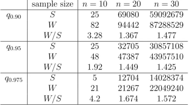
hence, it is one of most important cases. Its asymptotic squared bias, variance, and AM SE for some fixed points x0 are listed in Table 1, where we have omitted terms in powers of h.

Hb and He represent those values of H(xb ₀) and H(xe ₀), and every x₀ is each ε-th quantile of Γ(p,100). The kernel is an Epanechnikov one with A_2,1 = 1/5, A_0,2 = 3/10, and h = n⁻^1/5. The coeﬃcients n⁻^4/5 have been omitted.

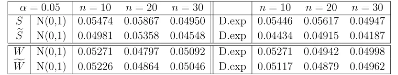
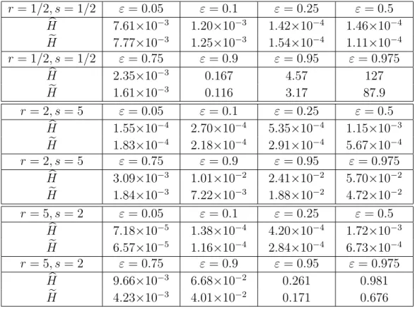
The Weibull distributionW(q, σ) is also important in survival analysis because the hazard ratio is proportional to the polynomial degree (q−1); that is, H(x) = qσ^qx^q⁻¹. W(1, σ) is the exponential distribution. The beta distribution is often used to describe a distribution whose support is finite, and it has plentiful shapes. Tables 2, 3, and 4 give the least AM SE values usingh^∗ orh^∗∗(in Section 2.2), whereHb and He stand for theAM SE values ofH(xb ₀) and H(xe ₀). Every x₀ is each ε-th quantile of Γ(p,100), W(q,100), or (100×B(r, s)). The tables demonstrate that the proposed estimator Hb performs asymptotically better in most cases of the gamma Γ(p,100). Moreover, the asymptotic performance of our estimator in the Weibull distribution cases is good and comparable to that of the beta cases.

(17)

Table 1: AsymptoticBias², V ar and AM SE when F is gamma

Bias² V ar AM SE Bias² V ar AM SE

p= 1/2,ε = 0.05 p= 1/2, ε= 0.1

Hb 7.22×10⁻² 4.01×10⁻² 0.112 8.24×10⁻⁵ 2.11×10⁻² 2.11×10⁻² He 6.53×10⁻² 4.22×10⁻² 0.107 6.72×10⁻⁵ 2.33×10⁻² 2.34×10⁻²

p= 1/2,ε = 0.25 p= 1/2, ε= 0.5

Hb 1.33×10⁻⁸ 9.52×10⁻³ 9.52×10⁻³ 2.36×10⁻¹¹ 5.65×10⁻³ 5.65×10⁻³ He 7.74×10⁻⁹ 1.27×10⁻² 1.27×10⁻² 6.83×10⁻¹² 1.13×10⁻² 1.13×10⁻²

p= 1/2,ε = 0.75 p= 1/2, ε= 0.9

Hb 5.35×10⁻¹³ 4.29×10⁻³ 4.29×10⁻³ 1.69×10⁻¹⁵ 3.76×10⁻³ 3.76×10⁻³ He 6.00×10⁻¹⁴ 1.72×10⁻² 1.72×10⁻² 2.93×10⁻¹⁵ 3.76×10⁻² 3.76×10⁻²

p= 1/2,ε = 0.95 p= 1/2, ε= 0.975

Hb 1.01×10⁻¹² 3.58×10⁻³ 3.58×10⁻³ 1.47×10⁻¹¹ 3.46×10⁻³ 3.46×10⁻³ He 6.93×10⁻¹⁶ 7.16×10⁻² 7.16×10⁻² 2.33×10⁻¹⁶ 0.139 0.139

Bias² V ar AM SE Bias² V ar AM SE

p= 10, ε= 0.05 p= 10, ε= 0.1

Hb 2.49×10⁻¹⁸ 1.56×10⁻⁴ 1.56×10⁻⁴ 2.16×10⁻¹⁸ 2.55×10⁻⁴ 2.55×10⁻⁴ He 7.16×10⁻¹⁹ 1.64×10⁻⁴ 1.64×10⁻⁴ 1.73×10⁻²¹ 2.83×10⁻⁴ 2.83×10⁻⁴

p= 10, ε= 0.25 p= 10, ε= 0.5

Hb 2.61×10⁻¹⁸ 4.77×10⁻⁴ 4.77×10⁻⁴ 1.37×10⁻¹⁷ 7.72×10⁻⁴ 7.72×10⁻⁴ He 2.40×10⁻¹⁸ 6.36×10⁻⁴ 6.36×10⁻⁴ 7.91×10⁻¹⁸ 1.54×10⁻³ 1.54×10⁻³

p= 10, ε= 0.75 p= 10, ε= 0.9

Hb 2.84×10⁻¹⁶ 1.07×10⁻³ 1.07×10⁻³ 1.19×10⁻¹⁴ 1.32×10⁻³ 1.32×10⁻³ He 1.05×10⁻¹⁷ 4.28×10⁻³ 4.28×10⁻³ 9.83×10⁻¹⁸ 1.32×10⁻² 1.32×10⁻²

p= 10, ε= 0.95 p= 10, ε = 0.975

Hb 1.84×10⁻¹³ 1.45×10⁻³ 1.45×10⁻³ 2.75×10⁻¹² 1.56×10⁻³ 1.56×10⁻³ He 8.70×10⁻¹⁸ 2.90×10⁻² 2.90×10⁻² 7.58×10⁻¹⁸ 6.24×10⁻² 6.24×10⁻²

(18)

Table 2: AM SE values when F is gamma and h=h^∗ or h^∗∗

p= 1/2 ε= 0.05 ε = 0.1 ε= 0.25 ε= 0.5 Hb 7.44×10⁻² 1.14×10⁻² 1.06×10⁻³ 1.97×10⁻⁴ He 7.60×10⁻² 1.19×10⁻² 1.20×10⁻³ 2.67×10⁻⁴ p= 1/2 ε= 0.75 ε = 0.9 ε= 0.95 ε = 0.975

Hb 7.40×10⁻⁵ 2.11×10⁻⁵ 7.26×10⁻⁵ 1.21×10⁻⁴ He 1.45×10⁻⁴ 1.48×10⁻⁴ 1.86×10⁻⁴ 2.54×10⁻⁴ p= 10 ε= 0.05 ε = 0.1 ε= 0.25 ε= 0.5

Hb 4.48×10⁻⁷ 6.45×10⁻⁷ 1.11×10⁻⁶ 2.26×10⁻⁶ He 3.64×10⁻⁷ 1.68×10⁻⁷ 1.37×10⁻⁶ 3.53×10⁻⁶ p= 10 ε= 0.75 ε = 0.9 ε= 0.95 ε = 0.975

Hb 5.39×10⁻⁶ 1.34×10⁻⁵ 2.51×10⁻⁵ 4.57×10⁻⁵ He 8.46×10⁻⁶ 2.05×10⁻⁵ 3.76×10⁻⁵ 6.75×10⁻⁵

Table 3: AM SE values when F is weibull and h=h^∗ or h^∗∗

q= 1/2 ε= 0.05 ε= 0.1 ε= 0.25 ε= 0.5 Hb 4.11×10⁻² 5.68×10⁻³ 3.85×10⁻⁴ 4.25×10⁻⁵ He 4.20×10⁻² 5.93×10⁻³ 4.30×10⁻⁴ 5.50×10⁻⁵ q= 1/2 ε= 0.75 ε= 0.9 ε= 0.95 ε= 0.975

Hb 9.22×10⁻⁶ 3.31×10⁻⁶ 3.59×10⁻⁷ 2.67×10⁻⁶ He 1.53×10⁻⁵ 8.61×10⁻⁶ 7.68×10⁻⁶ 7.90×10⁻⁶ q = 10 ε= 0.05 ε= 0.1 ε= 0.25 ε= 0.5

Hb 1.20×10⁻⁴ 2.65×10⁻⁴ 9.00×10⁻⁴ 3.40×10⁻³ He 1.11×10⁻⁴ 2.23×10⁻⁴ 4.79×10⁻⁴ 2.34×10⁻³ q = 10 ε= 0.75 ε= 0.9 ε= 0.95 ε= 0.975

Hb 1.38×10⁻² 5.49×10⁻² 0.135 0.309 He 1.33×10⁻² 5.96×10⁻² 0.153 0.360

(19)

Table 4: AM SE values when F is beta and h=h^∗ or h^∗∗

r= 1/2, s= 1/2 ε= 0.05 ε = 0.1 ε= 0.25 ε= 0.5 Hb 7.61×10⁻³ 1.20×10⁻³ 1.42×10⁻⁴ 1.46×10⁻⁴ He 7.77×10⁻³ 1.25×10⁻³ 1.54×10⁻⁴ 1.11×10⁻⁴ r= 1/2, s= 1/2 ε= 0.75 ε = 0.9 ε= 0.95 ε = 0.975

Hb 2.35×10⁻³ 0.167 4.57 127

He 1.61×10⁻³ 0.116 3.17 87.9

r = 2, s= 5 ε= 0.05 ε = 0.1 ε= 0.25 ε= 0.5 Hb 1.55×10⁻⁴ 2.70×10⁻⁴ 5.35×10⁻⁴ 1.15×10⁻³ He 1.83×10⁻⁴ 2.18×10⁻⁴ 2.91×10⁻⁴ 5.67×10⁻⁴ r = 2, s= 5 ε= 0.75 ε = 0.9 ε= 0.95 ε = 0.975

Hb 3.09×10⁻³ 1.01×10⁻² 2.41×10⁻² 5.70×10⁻² He 1.84×10⁻³ 7.22×10⁻³ 1.88×10⁻² 4.72×10⁻² r = 5, s= 2 ε= 0.05 ε = 0.1 ε= 0.25 ε= 0.5

Hb 7.18×10⁻⁵ 1.38×10⁻⁴ 4.20×10⁻⁴ 1.72×10⁻³ He 6.57×10⁻⁵ 1.16×10⁻⁴ 2.84×10⁻⁴ 6.73×10⁻⁴ r = 5, s= 2 ε= 0.75 ε = 0.9 ε= 0.95 ε = 0.975

Hb 9.66×10⁻³ 6.68×10⁻² 0.261 0.981 He 4.23×10⁻³ 4.01×10⁻² 0.171 0.676

(20)

2.4 Appendices: Some Proofs

Proof of Theorem 1

For simplicity, we will use the following notation, t(z) =

∫ _z

−∞

F(u)du, T(z) =

∫ _z

−∞

t(u)du,

M(z) = z−t(z) and m(z) =M^′(z) = 1−F(z).

To begin with, we consider the following stochastic expansion of the direct estimator:

H(xb ₀)

= 1

h

∫ _∞

−∞

k

(M(w)−M(x0) h

)

dFn(w) + 1

h²

∫ _∞

−∞

k^′

(M(w)−M(x₀) h

)

{[t(w)−t_n(w)]−[t(x₀)−t_n(x₀)]}dF_n(w) + 1

h³

∫ _∞

−∞

k^′′

(M(w)−M(x₀) h

)

{[t(w)−t_n(w)]−[t(x₀)−t_n(x₀)]}²dF_n(w) +· · ·

= J₁+J₂+J₃+· · · (say).

The main term of the expectation ofH(xb ₀) is given byJ₁, as we will show the later. Since J₁ is a sum ofi.i.d. random variables, the expectation can be obtained directly:

E[J1] = E [1

h

∫ _∞

−∞

k

(M(w)−M(x₀) h

)

dFn(w) ]

= 1

h

∫ _∞

−∞

k

(M(w)−M(x₀) h

)

f(w)dw

=

∫ _∞

−∞

k(u) [ f

1−F ]

(M⁻¹(M(x₀) +hu))du

=

[ f 1−F

]

(x₀) + h² 2 A_2,1

[(1−F){(1−F)f^′′+ 4f f^′}+ 3f³ (1−F)⁵

]

(x₀) +O(h⁴).

Combining the following second moment, 1

h²

∫ _∞

−∞

k²

(M(w)−M(x₀) h

)

f(w)dw

= 1

h

∫ _∞

−∞

k²(u) [ f

1−F ]

(M⁻¹(M(x0) +hu))du

= 1

h f

1−F(x0)A0,2+O(n⁻¹),

(21)

we get the variance,

V[J₁] = 1 nh

[ f 1−F

]

(x₀)A_0,2+O(n⁻¹).

Next, we consider the following representation of J₂ J₂ = 1

n²h²

∑n i=1

∑n j=1

k^′

(M(X_i)−M(x₀) h

)

Q(X_i, X_j), where

Q(x_i, x_j) = [t(x_i)−(x_i−x_j)₊]−[t(x₀)−(x₀ −x_j)₊].

Using the conditional expectation, we get the following equation:

E[J₂] = 1 nh²

∑n j=1

E [

k^′

(M(X_i)−M(x₀) h

)

Q(X_i, X_j) ]

= 1

nh²E [

k^′

(M(X_i)−M(x₀) h

) E

[ _n

∑

j=1

Q(X_i, X_j)X_i ]]

= 1

nh²E [

k^′

(M(X_i)−M(x₀) h

)

{t(X_i)−[t(x₀)−(x₀−X_i)₊]} ]

= 1

nh

∫ _∞

−∞

k^′(u){

t(M⁻¹(M(x₀) +hu))−t(x₀) + (x₀−M⁻¹(M(x₀) +hu))₊}

× f

1−F(M⁻¹(M(x₀) +hu))du

= 1

nh

∫ _∞

−∞

k^′(u)O(hu) f

1−F(x₀)du=O (1

n )

. Next, we have

J₂² = 1 n⁴h⁴

∑n i=1

∑n j=1

∑n k=1

∑n ℓ=1

k^′

(M(X_i)−M(x₀) h

) k^′

(M(X_k)−M(x₀) h

)

×Q(Xi, Xj)Q(Xk, Xℓ)

= 1

n⁴h⁴

∑n i=1

∑n j=1

∑n k=1

∑n ℓ=1

D(i, j, k, ℓ) (say).

After taking the conditional expectation, we find that if all of the (i, j, k, ℓ) are diﬀerent, E[D(i, j, k, ℓ)] = E[E{D(i, j, k, ℓ)|X_i, X_k}] = 0,

(22)

and

E[D(i, j, k, ℓ)] = 0 (if i=j and all of (i, k, ℓ) are different), E[D(i, j, k, ℓ)] = 0 (if i=k and all of (i, j, ℓ) are different), E[D(i, j, k, ℓ)] = 0 (if i=ℓ and all of (i, j, k) are different),

the term in whichj =ℓ and all of the (i, j, k) are diﬀerent is the main term ofE[J₂²]. Ifj =ℓ and all of the (i, j, k) are diﬀerent, we have

E[D(i, j, k, ℓ)]

= n(n−1)(n−2) n⁴h⁴ E

[ k^′

(M(X_i)−M(x₀) h

) k^′

(M(X_k)−M(x₀) h

)

×Q(X_i, X_j)Q(X_k, X_j) ]

.

Using the conditional expectation of Q(X_i, X_j)Q(X_k, X_j) given X_i and X_k, we find that E

[ E

{

Q(X_i, X_j)Q(X_k, X_j)X_i, X_k }]

= E

[

t(Xi)t(x0) +t(Xk)t(x0)−t²(x0) + 2T(x0)−t(Xi)t(Xk)

−(x+Xi−2 min(x, Xi))t(min(x, Xi))−2T(min(x, Xi))

−(x+X_k−2 min(x, X_k))t(min(x, X_k))−2T(min(x, X_k)) +(X_i+X_k−2 min(X_i, X_k))t(min(X_i, X_k)) + 2T(min(X_i, X_k))

] . Therefore, the entire expectation of the last row is

E [

k^′

(M(X_i)−M(x₀) h

) k^′

(M(X_k)−M(x₀) h

)

×(X_i+X_k−2 min(X_i, X_k))t(min(X_i, X_k)) + 2T(min(X_i, X_k)) ]

=

∫ _∞

−∞

[∫ w

∞

k^′

(M(z)−M(x₀) h

) k^′

(M(w)−M(x₀) h

)

× {(−z+w)t(z) + 2T(z)}f(z)dz +

∫ _∞

w

k^′

(M(z)−M(x₀) h

) k^′

(M(w)−M(x₀) h

)

× {(z−w)t(w) + 2T(w)}f(z)dz ]

f(w)dw.

カーネル平滑化統計量に基づくノンパラメトリック 推測