Computational study on prediction and reduction of aerodynamic noise from fans

(1)

Computational study on prediction and reduction of aerodynamic noise from fans

著者 LIM Tae‑Gyun

著者別名林泰均

その他のタイトルファンから生じる空力騒音の予測と低減に関する計算的研究

page range 1‑154

year 2018‑03‑24 学位授与番号 32675乙第229号学位授与年月日 2018‑03‑24

学位名博士(工学)

学位授与機関法政大学 (Hosei University)

URL http://doi.org/10.15002/00014768

(2)

Doctoral Dissertation Reviewed by Hosei University

Computational study on prediction and reduction of aerodynamic noise from fans

（ファンから生じる空力騒音の予測と低減に関する計算的研究）

Tae-Gyun Lim

林泰均

(3)

Supervisor : Professor Gaku Minorikawa, Hosei University

(4)

Abstract

i

Abstract

Turbomachinery is machinery device in which energy is delivered either to or from fluid that is continuously moving due to action of moving blades. Performance and flow noise are two major indices for evaluation of turbomachinery. In terms of energy transfer, researches on performance of turbomachinery have been conducted since long time ago; and these researches for performance improvement are still ongoing currently.

In addition, flow noise produced by turbomachinery came to the fore as turbomachinery has been used in various fields and everyday life closely and frequently. Especially, consumers’ demand on improvement in affective quality has been increased and regulation on noise has been being reinforced due to damages and adverse effects caused by noise. Therefore, development of high performance and low noise turbomachinery is highly required.

Meanwhile, experimental methods have been used to develop low noise turbomachinery; however, the experimental methods solely are not sufficient to achieve such aim since measuring in small turbomachinery is challenging. Hence, prediction technique, to which the numerical analysis method that yields complementary effects in combination with the experimental methods is applied, is required.

This study was conducted with the aim of applying numerical analysis method for noise reduction in turbomachinery. Therefore, three-dimensional unsteady Navier- Stokes equations were solved to simulate the flow field. Turbulence models used to predict the flow field were SST k–ω model that provides outstanding simulation of separation and adverse pressure gradient in boundary layer and LES model that presents excellence in turbulence intensity modeling, respectively. Computational Aeroacoustics (CAA) used to predict the flow noise in this study was acoustic analogy that is one of the hybrid methods; and the acoustic analogy is the method analyzing unsteady flow field by using Computational Fluid Dynamics (CFD) and then predicting noise by using the information of unsteady flow field obtained from the results of CFD simulation. To conduct acoustic analogy, Lowson equation, which can be used to predict sound pressure for point force that is moving in a free field, was calculated. Despite of disadvantage that influence of an object including scattering, diffraction, and reflection

(5)

Abstract

ii

within acoustic field is difficult to be considered, this method that directly reduces noise sources was able to be drawn since the locations of the noise source can be seen by numerical approach. Because predicting the location of the noise source is able to figure out the unsteady flow which causes the noise. As a result, the reduction method of flow- induced noise in this study is to find the way to reduce or remove the unsteady flow generating the noise, based on CAA and CFD.

In order to indicate the location of the noise source, “Aeroacoustic source strength, A_st” was defined and compared with the location of the noise source measured by the acoustic camera to which beamforming technology is applied; and they were agreed qualitatively well each other.

Due to miniaturization of electronics and maintenance of fan performance, whereas size of fan is getting smaller, the rotational speed of it getting higher. In this study following the current trend, three fans with each other different type were used for adopting numerical method to noise reduction; ⅰ) a small axial fan of rotor’s diameter D

= 0.166 m and a rotation speed 2860 rpm with circular shroud, ⅱ) a small axial fan of rotor’s diameter D = 0.076 m and a rotation speed 7000 rpm with square-type shroud used in a rack mount server computer, ⅲ) a small centrifugal fan with rotor’s diameter D = 0.032 m and a rotation speed 10460 rpm used as a cooling fan in portable home electronics such as a small laptop computer. The noise of each type fan was predicted and compared with the measured noise. The predicted noise and measured noise presented agreement in tonal noise of the blade passing frequency (BPF) and its harmonic frequencies and in the broadband noise at low frequency. Although the broadband noise at high frequency was somewhat different due to random broadband noise, the shapes for noise reduction were able to be drawn effectively by predicting the location of the noise sources. Low noise models suggested for noise reduction provided the result of noise reduction from the prediction and specific noise level was used to evaluate the noise reduction considering the changes in fan performance.

In case of the axial flow fan with circular shroud, the interaction between the rotating rotor blades and the flow separated from the inlet of the shroud was found to be the major cause of the noise through the analysis on the location of the noise sources and unsteady flow field. Consequently, reduction of the flow noise was predicted by correcting the shape of the shroud inlet.

(6)

Abstract

iii

In the small axial flow fan installed in the rack mount server computer, the tonal noise occurring by irregular clearance between the blade tip and the shroud due to the square- shaped shroud was well predicted. In addition, coherence analysis was conducted to identify the relationship between the surface pressure fluctuation due to the flow and the sound pressure predicted from the microphone. As a result, the correlation for each frequency was well presented.

For a centrifugal fan that is used as a cooling fan in home electronics such as a portable small laptop computer, the flow structure of the centrifugal fan was simulated by setting the condition to be analogous to the operating condition within the actual product. And then the reduction of the flow noise was predicted by correcting the tip of the impeller blades based on the location of the noise sources.

This study aimed to apply the method of numerical analysis to the noise reduction in turbomachinery. For this, the unsteady flow field was analyzed, the result of noise prediction obtained from the flow filed information was compared and validated, and the location of the noise sources and the structure of the flow field causing the noise were understood; hence, the low noise design was able to be drawn effectively and properly. In this study, the reduction of the flow noise was successfully achieved by adopting the method of numerical analysis and the flow noise of the fan that were improved for noise reduction was predicted to be reduced by 0.8 and 3.7 dB, respectively.

(7)

Table of Contents

iv

Nomenclature

A_st : aeroacoustic source strength

a₀ : speed of sound

C_s : Smagorinsky model constant

D : diameter of the rotor

dB : decibel

F : force, blending function

G : Green’s function, filter function

H : head of the impeller

Hn : helicity

Ksa : specific noise level

L : length

M : Mach number

n : unit normal vector

p : pressure, acoustic pressure

Q : strength of point source, flow rate r : vector from source to observer Re : Reynolds number

S_ : source term

T : torque, Lighthill stress tensor

t : time

V : angular velocity vector

Greek letters

 : delta function

 : dependant variable

 : density

 : diffusion coefficient

μ : viscosity coefficient

τ : shear stress, time

(10)

Nomenclature

vii

Subscript

fluid : caused by the fluid flow

ref : reference

ret : quantity evaluated at the retarded time SGS : Sub-Grid Scale

Symbol

 : partial derivative

∆ : filter size

(11)

List of figures

viii

List of figures

Figure 1-1 Classification of fluid machinery and examples of turbomachines Figure 1-2 Turbine module of a modern turbofan jet engine

Figure 1-3 Various noise sources generated from fan

Figure 1-4 Computational Aeroacoustics(CAA) methodology

Figure 1-5 Comparison of slip factors with some test results for radial bladed impellers

Figure 1-6 Relative stream surfaces and intersecting S1 and S2 surfaces in a blade row

Figure 1-7 Control surface and deviation of dynamic characteristics

Figure 1-8 Axial distributions of mass-flow-averaged entropy and entropy generation rate for datum nozzle guide vane (NGV) design

Figure 1-9 Temporal variation of the flow field for s/D0 = 0.01 and s/D0 = 0.005 at three time steps

Figure 1-10 Calculated directional characteristic for the fundamental tone Figure 1-11 Effect of impeller with sloping blades

Figure 1-12 Disturbance vorticity contours at different instants in one period

Figure 1-13 Unsteady behavior of vortex core structures colored with normalized helicity

Figure 1-14 Fan sound power spectra; measured (——), SEM (‐‐‐‐‐) and LES(───) Figure 1-15 Power spectra of volute pressure fluctuations in pascals (experiment,

upper side; 3D-numerical simulation, bottom side)

Figure 1-16 Schematic diagram of wrap angle, simulated SPL, and comparison of the simulated and measured overall SPLs

Figure 1-17 Comparison of the predicted and measured sound pressure levels

Figure 2-1 Comparison of control volume formulations used in the finite volume method

Figure 2-2 SIMPLE algorithm

Figure 2-3 Control volume within a two-dimensional turbulent shear flow Figure 2-4 Definitions of the variables

(12)

List of figures

ix

Figure 2-5 Comparison of surface meshes used for CAA

Figure 2-6 Schematic diagram of the simulation for prediction of the noise Figure 2-7 Comparison of sound sources between experiment and CAA Figure 3-1 Measuring points for pressure fluctuations

Figure 3-2 Schematic diagram of a microphone setup Figure 3-3 Main dimensions of the axial flow fan Figure 3-4 Experimental setup for noise measurement

Figure 3-5 Location of the microphone for noise measurement Figure 3-6 Perspective view of fan and its shape

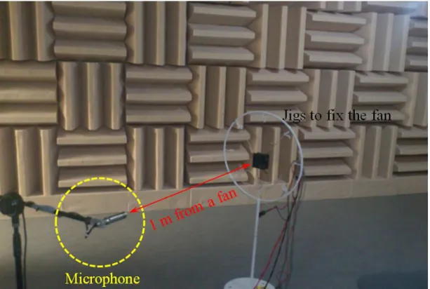
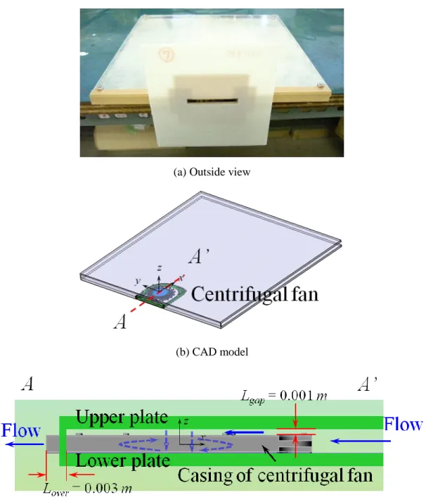
Figure 3-7 Photo of experimental set-up to measure the noise Figure 3-8 Main dimensions of a small centrifugal fan

Figure 3-9 Experimental setup and schematic diagram of flow channel and a small centrifugal fan

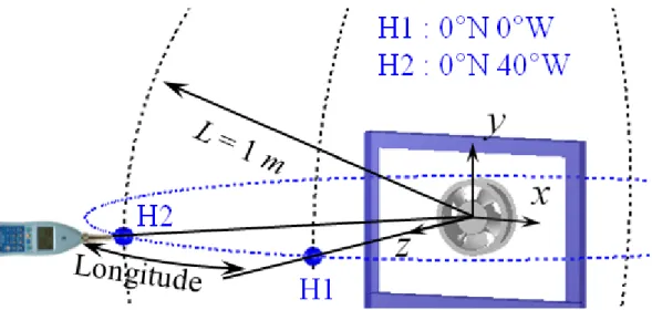
Figure 3-10 Microphone location for noise measurement

Figure 3-11 Detailed description of computational domain, boundary conditions and rotating frame

Figure 3-12 Computational grids

Figure 3-13 Computational domain and detail view of rotating frame Figure 3-14 Computational grids used to simulate the flow field

Figure 3-15 Computational domain, boundary conditions and rotating frame in detail

Figure 3-16 Computational grids for simulation of a centrifugal fan Figure 4-1 Fluctuation of static wall pressure on the strut of the shroud

Figure 4-2 Comparison of aeroacoustic sound spectra obtained by the numerical simulation and the experimental measurement

Figure 4-3 Distribution of the aeroacoustic source strength in Base model Figure 4-4 Distribution of the static wall pressure on the rotor of Base model Figure 4-5 Distribution of the vorticity at iso-surface of the helicity and the static

pressure at cross-section depending on time Figure 4-6 Comparison of the shroud shapes between models

Figure 4-7 Comparison of the aerodynamic sound spectra between models Figure 4-8 Distribution of the vorticity and the static pressure at t = 0.288647 sec

(13)

List of figures

x

Figure 4-9 Distribution of the aeroacoustic source strength in low noise models Figure 5-1 Distribution of relative velocity and velocity vector

Figure 5-2 Vorticity distribution on the cylindrical surface at r/rfan = 1.0000 Figure 5-3 Static pressure and velocity magnitude distribution

Figure 5-4 Velocity magnitude distribution depending on time at cylindrical surface r/r_fan = 1.0000

Figure 5-5 Comparison of aeroacoustic sound spectra obtained by numerical simulation and experimental measurement

Figure 5-6 Aeroacoustic source strength distribution

Figure 5-7 Coherence analysis between sound pressure and static pressure

Figure 6-1 Time-dependent static pressure distribution at two points on the inner casing

Figure 6-2 Distribution of static wall pressure on the inner casing Figure 6-3 z-directional velocity distribution on the zx plane with y = 0

Figure 6-4 Distribution of flow properties and streamline at z = -0.00145 m and t = 0.073996 sec

Figure 6-5 Vorticity distribution depending on time

Figure 6-6 Comparison of aerodynamic sound spectra of Base model Figure 6-7 Aeroacoustic source strength distribution of Base model Figure 6-8 Modification of impeller shapes for low noise

Figure 6-9 Comparison of aerodynamic sound spectra between Base model and modified impeller models

Figure 6-10 Vorticity distribution of r/r_fan = 1.00625 and t = 0.074252 sec Figure 6-11 Aeroacoustic source strength distribution in low noise models

(14)

List of tables

xi

List of tables

Table 4-1 Specific noise level between axial flow fans Table 6-1 Specific noise level between centrifugal fans

(15)

Chapter 1. General introduction and literature review

1

Chapter 1. General introduction and literature review

1.1 Background

Turbomachines are defined as all those devices which exchange energy either to, or from, a continuously flowing fluid through the dynamic motion of one or more moving blade rows. The word “turbo” or “turbinis” is from Latin origin and implies that which spins or whirls around [1]. Especially, the rotating blade row changes the pressure of the fluid by either doing work on the fluid (as a pump) or having work done on the blade row by the fluid (as a turbine), depending upon the purpose required of the machine [2].

The fan with the purpose of air conditioning was invented by Ding Huan who was a master artisan and engineer of Han Chinese in around the second century. The fan was in diameter of 3 m and manually rotated. Since then, Chinese in dynasty era used fan more frequently and they sometimes used water power to rotate fans [3]. The first rotating fan used in Europe was used to ventilate the inside of a mine during the 16th century as described by Georg Agricola (1494-1555) [3]. In 1727, Dr. John Théophile Desaguliers who was a British engineer designed the fan system for ventilation of mine in Westmorland by using the theory of chimney; and installed further improved device in Houses of Parliament in 1745. However, it was not utilized much due to difficulties in finding power source for operation of the fan. Afterwards, power-operated fans were begun to be used and the use was rapidly increased since the electric powered fan was invented at the end of 1800s. Now, fans are the most frequently used turbomachinery in everyday life as the one cannot find the field including the field of electric/electronic, automobile, and aviation where fans are not used. Examining the classification of fluid machinery, these can be divided by depending on the purpose of use such as displacement, kind of fluid, direction of energy or flow and so on. Figure 1-1 shows the classification of fluid machinery in detail. The turbomachines are classified by direction of energy as a pump and a turbine, can be divided again by direction of flow as axial flow type, radial flow type and mixed flow type, respectively. For instance, axial flow fans present uniform direction of the flow in general and are used where with high flow rate and small pressure difference. However, many axial flow fans were stacked in multi-layer for cases where large pressure difference and high flow rate are required

(16)

2

such as the engine of the air planes (Figure 1-2). Meanwhile, centrifugal fans have been used in vacuum cleaners, automobile HVAC and ventilation system for buildings where pressure difference rather than flow rate needs to be increased in small space. With the increased use of fans, issues of the fan noise that had not been considered before came to the fore. In particular, the sound source of the fan noise is in the space where people works in; hence, the radiation within the closed building and inside a room causes major noise issues. Predicting the noise source and the radiation patterns of the noise is essential since such noise has various influences including sleep interruption and the decrease in work efficiency.

In terms of energy, fans are the devices that transform the momentum energy to flow energy by delivering energy to flow through rotation of fan blades. In other words, the aim of a fan is to deliver energy to flow; hence, the primary interest is still in its performance. Various researches through experiments or numerical analysis have been conducted to improve fan performance up to date. Owing to the rapid development of calculation capacity of computers in the late 1990s, researches of numerical analysis on flow field of a fan have been being conducted particularly.

Interest in the noise caused by a fan is growing due to the increase in the use of fans as these are used in wide range of industrial field. For axial flow fans, the noise caused by airplanes was drawn attention relatively earlier as axial flow fans were used in the jet engines of airplanes. Consequently, a good number of results have been communicated by numerous researchers studied on the cause of noise and prediction methods in the 1960s and 1970s [4-7]. As a result, the fan noise mechanisms which explain the noise type generated by each source were summarized by Neise [8] in 1992 as following figure 1-3. Blade thickness noise or monopole noise is known, as giving a significant influence to fan noise only when the blade tip speed is over Mach number 0.5. The source of monopole noise is due to the volume displacement effect which generates repeatedly the disturbance in the flow field when the moving fan blade displaces fluid mass. The dipole noise is called loading noise and generates discrete and broadband noise. It can be explained as the noise generated by forces acting on the fluid. The quadrupole is related to Lighthill’s term and represents the sound radiation by fluctuating Reynolds stresses within fluid layers. According to Morfey [4], it becomes dominant issue only when the blade tip of rotational speed is greater than the Mach

(17)

3

number 0.8. It’s well-known to be generated typically by shear stresses.

Fans that are used in field of home appliances and automobiles are operated in subsonic domain; hence, the cause of the noise is different from the cause of the airplane’s noise and the size of the noise is relatively smaller than that caused by airplanes. Therefore, the practical noise reduction method through experiment has been studied. Since then, fans have been being widely used in closed area or near life space and thereby, consumers’ demand on affective quality has also been increased according to overall improvement in quality of products in the late 1990s. As a result, numerous researches adopting experiment or numerical analysis have been conducted. In addition, researches measuring and visualizing noise sources by utilizing beamforming are being conducted recently. Beamforming is one of microphone array locating technology. It can be considered as one of the usual acoustics visualizing method and is frequently used in industrial field to detect noise sources owing to its advantage of high speed, contactless, and high resolution. Researchers have been trying to find continuously the sound source, because it’s very important to find the place at where the source is located, in order to reduce the noise. However, only experimental methods are not enough to find and understand the unsteady flow field generating the noise. The numerical analysis is necessary to find and figure out the location of the sound source and the unsteady flow field generating the noise. Therefore, prior to adopting numerical analysis method for reduction of the flow noise, the locations of noise sources predicted by the numerical analysis in this study was compared with that measured by a equipment like a sound camera which has been developed based on a beamforming technology.

In summary so far, the noise of fans used in the industrial part except the aviation field was taken late relatively the customer’s attention and the main focus of the flow- induced noise in this study became the dipole noise. The application of the numerical analysis based on the main focus can provide the high feasibility for noise reduction in the turbomachines.

Meanwhile, the acoustics at dictionary is the branch of physics that deals with sound and sound waves in gases, liquids, and solids. Sound waves are classified by infrasound (f < 20 Hz), audible sound (20 Hz < f < 20 kHz) and ultrasound (20 kHz < f < 5 MHz) depending on frequency range. In audible sound, the classification of noise or music is

(18)

4

divided by whether giving people displeasure or not, when people listen to the sound.

Though the noise is divided as structure borne noise and airborne noise depending on the transmission medium of the sound waves, aeroacoustics was covered in this study.

The aeroacoustics is a branch that studies the noise generated by the turbulent flow, the periodically varying flow, the aerodynamic force interacting with a surface and so on.

Ffowcs Williams [9] defined that flow noise is the term used to describe the pressure fluctuations associated with unsteady flow, particularly turbulent flow. Therefore, the numerical method, which is called as Computational Aeroacoustics (CAA), as well as Computational Fluid Dynamics (CFD) to predict the unsteady flow field were required to understand or predict the flow noise in detail. CAA is a part of aeroacoustics to analyze the flow-induced noise generated in the flow field through numerical methods.

The numerical method predicting noise caused by flow is majorly classified into two kinds: direct method in which flow field and acoustic field that may be the noise source are analyzed simultaneously and hybrid method in which flow field that is the region of the noise source and acoustic field where the noise propagates are analyzed separately under the assumption that the influence of the acoustic field on the flow field is ignorable (Figure 1-4).

The direct method of the noise prediction is the method in which the sound pressure that causes noise is directly calculated by using the numerical method. However, the researches on this method were started to be conducted in the 1990s for the first time and have not been utilized wieldy even nowadays due to two reasons. The first reason is the physical causes including the differences in scale of the length between the flow field and the acoustic field and the difference in perturbation size between the flow field and the acoustic field. The second reason is caused by the demand of the numerical techniques requiring the high-order accuracy in the frequency-wavenumber domain as well as in the time-space domain.

The hybrid method of noise prediction analyzes the unsteady flow field, as the noise source region, by using Computational Fluid Dynamics (CFD) and then predicts noise propagation by utilizing acoustic analogy, boundary element method, and linear/nonlinear acoustic propagation equation. In this study, the hybrid method that has been known to be more efficient than the direct method was used. After obtaining unsteady flow field by utilizing CFD, the noise was predicted by using acoustic analogy

(19)

5

which is the one of hybrid methods. In general, it has been known that the appropriate model among numerous acoustic analogies should be applied by taking account of the environment where the flow noise of interest occurs because noise prediction based on acoustic analogy proposes a kind of approximate solution through the modeling of major noise sources. This study utilized the acoustic analogy derived from the Lighthill equation [10, 11]. The method using acoustic analogy allows obtaining accurate solution up to farther distance; however, the influence of scattering or reflection is difficult to be considered in case of having scattering or reflection due to an object when the object is inside the acoustic field. Notwithstanding this problem, the acoustic analogy can sufficiently propose the efficient and direct method for flow noise reduction by predicting the location of noise sources. The method of flow noise reduction with the numerical analysis is composed of the following procedures; first is the validation of the noise prediction value obtained from the aeroacoustic noise analysis utilizing acoustic analogy, second is the analysis on the locations of the predicted noise sources, third is the analysis and identification of unsteady flow causing the noise sources, and fourth is the prediction of the noise reduction by taking account of the shape that can reduce the unsteady flow related to the noise sources.

The fundamentals of aeroacoustic analogy was established by the sound wave equation in free space proposed by Lighthill in 1952 and 1954 and Curle [12] revised the equation so that it can be valid even in case of having object surface. In 1965, Lowson [13] induced the equation predicting sound pressure caused by moving point force and Ffowcs Williams and Hawkings [14] defined the flow noise sources occurring from moving objects with arbitrary velocity within the flow by expanding the acoustic analogy proposed by Lighthill and Curle.

In this study, acoustic field caused by the turbomachinery in a free space was predicted through the numerical analysis by using Lowson equation based on the information of unsteady flow field due to the turbomachinery. In addition, application of the numerical analysis to reduce the flow noise of the turbomachinery used practically was focused by describing the distribution of the noise sources through defining “Aeroacoustic source strength” from the result of the aeroacoustic noise analysis.

(20)

6

1.2 Literature review

In case of considering the operating fluid as gas, fans can be defined as the machineries with an impeller or a rotor that exerts mechanical work letting the gas to flow with arbitrary energy and is the turbomachinery that is the most frequently used in everyday life. The rotation velocity of a fan can be increased to maintain the performance depending on its operating condition, size, and shape. This complicates the flow field, increases the flow noise, and thereby causes serious problems in products.

Therefore, researches on fans were reviewed after classified into the flow analysis and the flow noise.

The flow analysis of a fan can be distinguished into the simple way analyzing the performance only and the method analyzing the flow field. Initially, only the performance of the impeller that supplies energy was studied in order to predict fan performance. Since then, the method that predicts the head of turbomachinery in a simple manner by using a velocity triangle with infinity blade theory was developed in the early 20^th century. Afterwards, the method that predicts performance based on finite blade theory where the slip factor was introduced was developed and numerous equations with regard to the slip factor have been studied. As shown in figure 1-5, Wiesner [15] provided the information for determination of slip factors within limitation of the mean radius ratio of the impeller in centrifugal impeller applications. Exceeding the limitation, an empirical correction was proposed.

Weissgerber and Carter [16], Takagi et al. [17] and Rathod and Donovan [18]

proposed a prediction method for centrifugal pumps in different types and with specific rotation speeds. Such method used a simple velocity triangle combined with several experimental equations and could predict somewhat accurate values for impellers in simple shape only in a narrow range near the best efficiency point, due to the causes of the inadequate flow modeling and without the consideration of all possible losses.

Nevertheless, they have been still used by many business entities.

Aforementioned method predicts the performance only; therefore, it does not offer information about the flow field including velocity or pressure on the blade surface. The origin of such method for the flow field analysis can be recognized as shown in figure 1-6 that Wu [19] divided the three-dimensional passage flow into S₁ and S₂ surface and calculated for each case in 1954. The method was further developed by Katsanis [20] in

(21)

7

1964 and numerous studies have been done based on Katsanis’s method. However, such methods were useful only when analyzing impellers at steady state and had the disadvantage that it was not able to be used when analyzing impellers at unsteady state or considering fans with the fixed parts including the casing and diffuser.

With the development of computers since the 1980s, studies on transient characteristics of two-dimensional inviscid unsteady state impeller had been conducted with the use of vortex panel by Tsukamoto and Ohashi [21], Imaichi, et al. [22], Tsukamoto, et al. [23], and Shoji and Ohashi [24]. Figure 1-7 shows the characteristics for the stopping transients through comparison of the calculated and measured data by Tsukamoto, et al. Afterwards, Kiya and Kusaka [25] conducted a numerical research on characteristics of the unsteady flow that was separated from the leading edge of the blade of the centrifugal impeller in the flow field of the two-dimensional inviscid incompressible fluid by using discrete vortex method in 1989. Owing to the rapid development of computer performance since the late 1990s, the three-dimensional flow field caused by the turbomachinery was simulated with the numerical analysis method and a good number of researches aiming for the improvement in fan performance have been conducted [26-28]. Panigrahi and Mishra [26] simulated the flow field near the airfoil produced by the angle of attack by using k–ε turbulence model in order to improve the efficiency of the axial fan for mine ventilation. In order to identify the effect of the vortex design and blade lean of the nozzle guide vane at turbine inlet, Zhang et al. [27] conducted the numerical analysis with SST k–ω turbulence model, analyzed the loss occurring in the guide vane according to the cause, and showed the distribution of each loss component based on the direction of the axis in figure 1-8.

Pogorelov et al. [28] conducted a large scale numerical analysis on the influence of the clearance in the tip leakage flow generated at an axial flow fan and analyzed the tip leakage vortex by using LES model. Figure 1-9 shows the unsteady flow field depending on time about each clearance.

Looking at a turbulence model used to simulate the flow field for fan performance prediction of the previous studies in recent years, Reynolds-Averaged Navier-Stokes (RANS) turbulence model established with the approach in terms of time-average is still being used. Because the reason presents excellent stability of convergence even though the number of grids used is small. Recently, the frequency of using LES model that

(22)

8

allows identification of turbulence eddy in various sizes by conducting direct analysis without physical modeling about turbulence eddy which is larger than a mesh size has been being increased.

The below is a brief review on acoustic analogy that is the fundamentals of the aeroacoustic noise. From the study reported by Lynam and Webb [29] in 1919, the acoustic noise by turbomachinery has been concentrated to predict the acoustic noise caused by rotor sand propellers of helicopters. Thereafter, his study by Gutin [30]

shown in figure 1-10 made a significant progress in the field of acoustic noise prediction. However, Gutin noise caused by the steady loading generating on propellers was not useful for fan noise prediction. In 1952, Lighthill [10] established aeroacoustics theory through conducting the dimensional analysis on the acoustic noise generation by using flow velocity and shape variables. Tyler and Sofrin [31] analyzed the noise radiation of rotating sources in a duct by simplifying the rotating fan as the acoustic source arranged to circumferential direction on the disk plane with using mode theories They reported that each blade number of rotor and stator is the most dominant factors in noise occurred by the interaction between the rotor and the stator. In 1965, Lowson induced the formula calculating the acoustic pressure produced by a moving point force [13]. Ffowcs Williams and Hawkings (FW-H) [14] drew an equation for a moving acoustic source by expanding the Curle’s study [12] which could not consider a moving acoustic source.

Meanwhile, the initial studies on the flow noise produced by the interaction between a rotating object such as a fan and the surrounding structures focused on the development of the method for noise reduction and noise prediction based on the experiments rather than the numerical analysis. The researches [32-37] related to the noise of centrifugal fans were more focused on the noise reduction by adjusting the increase of cut-off intervals, the lean of the impeller blades and cut-off edges, the mesh installation on leading and tailing edges of the impeller blades, and the placement of impeller blades asymmetrically. Figure 1-11 shows the effect of impeller with sloping blades in the noise reduction.

With the improvement of computational performance in 1990s, direct calculation based on Lighthill equation was enabled to predict the aeroacoustic noise. However, it is

(23)

9

still challenging to conduct the direct method of the noise field analysis due to the numerical methods requiring the high capacity grids and the accuracy of higher order.

Researches for noise prediction are still being conducted by utilizing CFD or taking the hybrid method yet [38-44].

In figure 1-12, Chen and Wu [38] showed that tonal noise of the blade passing frequency (BPF) and its harmonic frequencies is occurred by the interaction between a rotating rotor and a stationary structure through a vortex method based on Lagrangian frame. As shown in figure 1-13, Jang et al. [39-42] studied experimentally and numerically the influence of the tip leakage vortex generated by the tip clearance in an axial flow fan. They showed that reverse flow region was occurred repeatedly by periodic movement of the tip leakage vortex and the tip clearance near the reverse flow region caused the discrete frequency noise. Carlous et al. [43] studied on the noise prediction method for broadband noise of the low-pressure axial flow fan based on Semi-empirical noise prediction model (SEM) and LES models. The authors especially focused on the prediction of the interaction noise by ingested turbulence. As shown in figure 1-14, the method using SEM was easy to apply to the noise prediction; however, it was confirmed that it was not able to describe details in fan shapes and flow phenomenon such as separation. The method of the numerical analysis using LES model was good at predicting the noise influenced by the shape, the effect of the ingested turbulence on the sound sources, and fan noise; however, differences was found in broadband noise. Ballesteros-Tajadura et al. [44] conducted a numerical analysis for the unsteady flow to predict the noise from a radial flow fan and then predicted an acoustic field around the fan by using the FW-H equation and the surface pressure fluctuations on rotor and volute tongue obtained from the flow field. Finally, they measured sound pressure level (SPL) in experiment and compared it with the results obtained from the simulation in figure 1-15. They presented differences in prediction of the broadband noise and tonal noise, respectively. Scheita et al. [45]

showed in figure 1-16 that wrap angle in a small radial fan was clearly related to aerodynamics and flow noise. They also reported that an isolated impeller could improve the aerodynamic efficiency but did not generate the flow-induced noise radiation.

For more accurate noise prediction, consideration on the interaction between the sound

(24)

10

and the structures including scattering and diffraction was known to be required. To do this, the wave equation in which the structures are considered with the aid of FED and BEM should be solved. However, the two analysis methods require additional preprocess including appropriate surface grids and space grids for aeroacoustic noise analysis. Getting more accurate result for the noise field is important; however, predicting noise in a free field by utilizing the hybrid method was determined to be sufficient for application of the numerical method to the noise reduction in the turbomachinery. Hence, the noise field was predicted by using the hybrid method rather than the direct method with high load for aeroacoustic noise prediction and aeroacoustic analogy in a free field was used.

The aeroacoustic analogy analyzes the acoustic field by using the analytical solution for all of monopole, dipole, and quadrupole noise sources. However, most fans excluding the fans used in field of aviation are operated in supersonic domain with small Mach number (M). Neise reported the dipole noise source as the major noise source of the turbomachinery that are operated in supersonic domain and described the understanding on the noise source of a fan as shown in figure 1-3 [8]. And it was not easy to apply the FW-H equation to practical problems; hence, an easier calculation method using Lowson equation was proposed by Jeon and Lee [46]. The static wall pressure fluctuations of a body obtained after simulating the unsteady flow field are used for CAA calculation by this method [47-54]. Jeon [48], Jeon and Lee [49], and Jeon et al. [50] predicted the noise of centrifugal fan by using the two-dimensional discrete vortex method. In those studies, BPF tone noise was well agreed whereas there was somewhat large difference found in broadband noise. As shown in figure 1-17, the disagreement in broadband noise was determined to be caused by the difference between the complicated actual flow in three-dimensional shape and the two- dimensional flow analysis. Lim et al. [51, 52] predicted the noise of the turbomachinery by taking account of the three-dimensional shape and compared the prediction with the experimental value. In addition, the authors described the flow characteristics related on noise sources by analysing the locations of the noise sources. Lim et al. [53, 54] adopted the numerical analysis method for noise reduction in the turbomachinery by analysing the locations of the noise sources.

(25)

11

1.3 Methodology

This study was conducted with the focus on the application of the numerical analysis on the acoustic field for noise reduction in the turbomachinery. With this purpose, the acoustic field produced by the turbomachinery was predicted in a free space by using Lowson equation that predicts the acoustic field occurring by the moving point force based on the research result that the dipole is dominant in the acoustic field. The process of the numerical analysis on the unsteady flow field for application of Lowson equation was conducted in following sequence: steady state fluid analysis that minimizes the calculation time by creating the sketchy flow field that is produced by the turbomachinery in the semi-anechoic room, the unsteady state flow analysis for full development of the unsteadiness caused by the turbomachinery, and the unsteady flow field analysis to obtain the surface pressure fluctuation in the rotating part and fixed part by time during several rotations of the rotor. At the moment, the fluid properties were checked at arbitrary locations in order to fully develop the unsteadiness of the flow field.

For three-dimensional simulation of the flow field, the turbulence models used in steady state and unsteady state were SST k–ω that can predict the adverse pressure gradient on the surface of the blade and LES model that is excellent in modeling of the turbulence intensity, respectively.

The surface pressure fluctuations by time obtained from the flow field analysis and the noise spectrum predicted by aeroacoustic analogy were verified after comparing with the noise spectrum measured in the semi-anechoic room for each model. Through the comparison between the noise spectrums, good agreement in the tonal noise of the 1st BPF and its harmonic frequencies and in the broadband noise was shown at a low frequency range; however, difference was found from the broadband noise at high frequency. Such disagreement was determined to be caused by the random broadband noise. In general, random broadband noise is caused by various phenomena such as turbulent boundary layer, vortex shedding, flow separation, and tip vortex. However, the scattering influence by the turbulent boundary layer which was occurred from the trailing edge of blades was not considered in this study. As a result, such disagreement of prediction at high frequency range was caused by consideration of only the dipole.

Meanwhile, the location of the noise sources was described in validated result of the noise prediction by defining Aeroacoustic source strength (A_st) that can predict the

(26)

12

location of the noise source and the unsteady state flow producing the noise based on the location of the noise source was confirmed. Prior to this study, the feasibility of the prediction of the noise source location was verified through the comparison between the location measured by using an acoustic camera with beamforming technology and the location predicted by the numerical analysis.

In addition, the correlation between the sound pressure predicted from the microphone located 1 m apart from the turbomachinery and the surface pressure fluctuation by time obtained from each of the two points (bell mouth and strut) in the unsteady flow field were confirmed by conducting coherence analysis. It was able to confirm the difference in the flow field between the two points from the coherence analysis on the frequency.

The numerical analysis method was applied for the comparison of the numerically predicted value and the measured value of the flow noise in the turbomachinery, for understanding and analysis of unsteady state flow producing the noise based on the location of the noise source, for identification of the shape reducing the unsteady state flow causing the noise, and for the reduction of the flow noise in the turbomachinery.

1.4 Objectives of this study and outline

In Chapter 1, the motive, background, and purpose of the research were stated and literature review and method and range of the research were described.

In Chapter 2, the numerical analysis method for simulation of the flow field and that for prediction of the noise produced by the turbomachinery in a free space was described. The noise of the turbomachinery in a free space was calculated by using Lowson equation under the assumption that it is produced from the rotating parts (impeller and rotor) and fixed parts (shroud). However, the numerical analysis on surface pressure fluctuation acting on the rotating parts should be done first in order to calculate aeroacoustic noise. Therefore, the unsteady flow field was numerically analyzed as a preceding study for noise analysis and the method to obtain the information on the flow field was described. For prediction of the location of the noise source, the possibility of the prediction was confirmed in advance by comparing with the location of the noise source measured by the acoustic camera.

In Chapter 3, the experimental setup measuring the flow noise and the numerical setup for prediction of the flow noise were introduced. Details including the size of semi-

(27)

13

anechoic room for measuring the noise of the turbomachinery, the rotating speed, the location of the microphone, the conditions of the computational domain and boundary, the grid information, the convergence condition, and the time step were described.

In Chapter 4, the flow noise predicted was compared with that measured from the axial flow fan with cylindrical shroud and the unsteady state flow causing the noise was confirmed. In order to reduce the unsteady state flow causing the noise, the flow noise was reduced by correcting the shape of the shroud inlet. Degree of the noise reduction was compared by using specific noise level among all other indexes representing the changes in fan performance owing to the changes in the shape of the shroud inlet in this study.

Chapter 5 handles the prediction of the characteristics of the noise produced by a small axial flow fan for cooling. In particular, the tonal noise due to the shape of the square- type shroud and the locations of the related noise sources were predicted. In addition, the correlation between the flow field and the noise was confirmed by conducting coherence analysis on the surface static pressure fluctuation obtained from each of bell mouth and strut, the two points on the shroud, and sound pressure fluctuation that was predicted from the microphone location.

In Chapter 6, the flow characteristics and noise of the centrifugal fan that has been used for cooling in portable home electronics including small laptops and ultrabooks were predicted. For this, the centrifugal fan that is installed between the two thin square flat boards was studied in order to give the condition that is analogous to the fan operated inside a product. Based on the result of the numerical analysis, the blade tip of the impeller was corrected to reduce the unsteady flow related to the flow noise and the aeroacoustic noise in corrected impeller shape was predicted. In addition, the specific noise level was used to compare the noise reduction of the centrifugal fan considering the fan performance.

Chapter 7 described the summary of the results obtained in this study.

1.5 Summary

The sound is divided as unpleasant noise and pleasant one. Though the noise is also classified by structure borne and airborne depending on the transmission medium of the sound waves, aeroacoustics was only considered in this study. The flow-induced noise is

(28)

14

generated by the turbulent flow, aerodynamic force interacting between surfaces, the periodically vary flow, and so on. Especially, the flow noise defined by Ffowcs Williams [9] is known as the term used to describe the pressure fluctuations associated with unsteady flow, particularly turbulent flow. Therefore, understanding and analyzing the unsteady flow field in detail have been being required obligatorily to predict and reduce the flow noise. In other words, the flow noise is related closely to the fluid dynamics and the acoustics.

Meanwhile, as fans have been used in wide range of the industrial field, the fan performance and the noise generated from fans have been taken attention. Looking at the study by Neise [8] and fan noise mechanism to explain the noise type, the noise of fans used in the industrial field except the aviation part is known that dipole is the dominant noise source. Numerous studies using experimental methods have been conducted to reduce the noise. But due to miniaturization of a product, the numerical analysis has been asked to figure out the unsteady flow field in the inside of the product in detail and to predict the sound source. It means that finding the relationship between the unsteady flow field and the sound source is important. Therefore, the objective in this study is to apply and use the numerical method in order to find the relationship between unsteady flow field and the sound source and conduct the noise reduction.

The detailed contents for accomplishing the purpose of this study are as follows. In this chapter, the background, literature reviews about the flow-induce noise, methodology, objectives and outlines of this study were reviewed for introduction of turbomachines. Chapter 2 mentioned the numerical method for simulation, and Chapter 3 described the setup about experiment and simulation, respectively. By considering fans installed in the electronic products, three different type fans were used for applying the numerical analysis to noise reduction. Chapter 4, 5 and 6 showed validation of predicted results obtained from CAA, and then low noise models about an axial flow fan and a centrifugal fan were suggested and provided the noise reduction through numerical analysis. In Chapter 7, the results obtained in this study were summarized.

(29)

15

Fig. 1-1 Classification of fluid machinery and examples of turbomachines [1]

(30)

16

Fig. 1-2 Turbine module of a modern turbofan jet engine [1]

(31)

17

Fig. 1-3 Various noise sources generated from fan

(32)

18

Fig. 1-4 Computational Aeroacoustics(CAA) methodology

(33)

19

Fig. 1-5 Comparison of slip factors with some test results for radial bladed impellers [15]

(34)

20

(a) Relative stream surface S1 and S2

(b) Intersecting S1 and S2 in a blade row

Fig. 1-6 Relative stream surfaces and intersecting S₁ and S₂ surfaces in a blade row [19]

(35)

21

(a) Control surface for considering pressure rise through cascade

(b) Deviation of dynamic characteristics from quasi-steady ones during stopping period Fig. 1-7 Control surface and deviation of dynamic characteristics [23]

(36)

22

Fig. 1-8 Axial distributions of mass-flow-averaged entropy and entropy generation rate for datum nozzle guide vane (NGV) design [27]

(37)

23

Fig. 1-9 Temporal variation of the flow field for s/D₀ = 0.01 and s/D₀ = 0.005 at three time steps [28]

(38)

24 (a) R = 0.7 R0

(b) R = 0.75 R0

Fig. 1-10 Calculated directional characteristic for the fundamental tone [30]

(39)

25

(a) Standard impeller (b) Modified impeller (blades sloping : 20°)

(c) Experimental results

Fig. 1-11 Effect of impeller with sloping blades [32]

(40)

26

Fig. 1-12 Disturbance vorticity contours at different instants in one period [38]

(41)

27

Fig. 1-13 Unsteady behavior of vortex core structures colored with normalized helicity [40]

(42)

28

Fig. 1-14 Fan sound power spectra; measured (——), SEM (‐‐‐‐‐‐) and LES(───) [43]

(43)

29 (a) At Point P06

(b) At Point P10

Fig. 1-15 Power spectra of volute pressure fluctuations in pascals (experiment, upper side; 3D-numerical simulation, bottom side) [44]

(44)

30

(a) Prototypes with wrap angle θ = 150° and θ = 228°

(b) Simulated SPL with different wrap angle (c) Overall SPL vs. mass flow rate Fig. 1-16 Schematic diagram of wrap angle, simulated SPL, and comparison of the

simulated and measured overall SPLs [45]

(45)

31

(a) Rotation speed : 26760 rpm

(b) Rotation speed : 29930 rpm

Fig. 1-17 Comparison of the predicted and measured sound pressure levels [50]

(46)

Chapter 2. Numerical analysis

32

Chapter 2. Numerical analysis

2.1 Computational Fluid Dynamics (CFD) 2.1.1 Fundamental equations

When dealing with thermal flow phenomenon of the fluid, equilibrium equations of the flow properties are used and these equations are usually presented as the differential equations. The differential equations can be expressed in general transport equation as below when setting the dependent variable as ф and using a tensor [55].

(2-1)

Equation (2-1) is composed of an unsteady term, a convection term, a diffusion term, and a source term. Here, ρ is the fluid density. Γ, the diffusion coefficient, and Sф, a source term, do not always have actual physical meaning. These can be interpreted as dependent variables including pressure, temperature, and velocity. Therefore, continuity equation can be obtained by assuming the dependent variable ф as 1, and Γ and Sф as 0 in equation (2-1), the general transport equation. Meanwhile, a momentum equation in Cartesian coordinate system in which the gravity is not considered is obtained by substituting ui that is the velocity component and uSj that is the velocity of the volume with moving boundary into ф, the dependent variable, and τ that is the shear stress and -

∂p/∂x that is the pressure gradient into Γ, the diffusion coefficient, and Sф, the source term, respectively, in general transport equation [56, 57].

(2-2)

In order to analyze the continuity equation and the flow around the moving object used in this study, Navier-Strokes equations can be presented into a simple tensor notation shown in below.

(2-3)

(47)

33

(2-4)

The i(i = 1, 2, 3), the subscripts in above equation, corresponds to the (x, y, z); hence, (u1, u2, u3) indicates (u, v, w) that is the notation according to three-dimensional Cartesian coordinate system of velocity and (x1, x2, x3) indicates (x, y, z).

2.1.2 Discretization method

After choosing the mathematical model predicting the flow field, discretization of the differentials equation should be performed as matching the grid point and the algebraic equations for ф, the dependent variable, in the chosen grid point are called discretized equations. The discretization method for differential equation is classified into Finite Difference Method (FDM), Finite Element Method (FEM), and Finite Volume Method (FVM). In FDM, the derivative term in the differential equation is expressed by using Taylor-series expansion. On structured grids, FDM is a very simple and effective method. In particular, it is easy to obtain a higher-order scheme in regular grids with the method. The disadvantages of FDM are the difficulties in maintaining the conservation and applying to complicate flow. FEM expresses the unknown as an approximation function of the required accuracy and determines the size of the coefficient for each small region by using weighted residual method. Finite element methods are relatively easy to analyze mathematically and can provide optimality properties for equations of certain types. The principal disadvantage, which is occurred by methods to uses unstructured grids, is that the matrices of the linearized equations are not as well structured as those for structured grids. As a result, it makes more difficult to find efficient solution methods [55, 56]. FVM is the discretizing method of differentiating the properties that are coming in and out across the surfaces composing the volume of the polyhedron after assuming that the physical quantity including velocity and pressure can be predicted at the center of the polyhedron. The FVM can accommodate any type of grid, so it is suitable for complex geometries. The grid defines only the control volume boundaries and need not be related to a coordinate system. The method is conservative by construction, so long as surface integrals, which represent convective and diffusive fluxes, are the same for the control volumes sharing the boundary. The

(48)

34

FVM approach is perhaps the simplest to understand and to program. All terms that need be approximated have physical meaning. The disadvantage of FVMs compared to FDMs is that methods of order higher than second are more difficult to develop in 3D [55, 56].

The fundamental discretizing method for the space in the solver used for numerical analysis of thermal flow in this study is the vertex-based FVM. Therefore, the discretization in this study is limited to that by FVM.

Figure 2-1 shows the vertex-based scheme used in this study and the cell-based scheme, respectively [58]. The vertex-based FVM used in CFD solver is the discretizing method by re-dividing the space with the vertex as the center rather than discretizing the properties by using the center of the space; hence, the method can differ by the way of composition of the control volume. In general, the median method in which the control volume is composited by connecting the center of the cell, the center of the surface, and the center of the edge is widely used [57]. In particular, a cell-centered scheme can be expected to result in a much larger number of unknowns while generating relatively simple stencils of fixed size. The vertex-based scheme, on the other hand, will result in a smaller number of unknowns with larger variable-size stencils. Because of the larger number of unknowns, cell-centered schemes generally incur larger overheads than vertex-based schemes on equivalent grids [59]. However, vertex-based scheme has been known that the convergency of the solution can be influenced when the quality of the imaginary plane created between the two nodes is not fair [60].

2.1.3 Pressure-correction method

Solution of the Navier-Stokes equations is complicated by the lack of an independent equation for the pressure, whose gradient contributes to each of the three momentum equations. Furthermore, the continuity equation does not have a dominant variable in incompressible flows. Mass conservation is a kinematic constraint on the velocity field rather than a dynamic equation. One way out of this difficulty is to construct the pressure field so as to guarantee satisfaction of the continuity equation [56]. In other words, the velocity that is composed of three vectors in the momentum equation occupies three unknowns while the pressure term that is a scalar occupies one unknown, resulting four unknowns in total. In order to obtain solutions for the four unknowns,