Chemiluminescence sensor for active control of combustion
Laurent ZIMMER and Shigeru TACHIBANA
Aeroengine Technnology Center, Institute of Aerospace Technology, JAXA
Abstract
The present document summarizes the different experiments done on active control by using chemiluminescence measurements. First a brief introduction on the chemical mechanisms that are responsible for chemiluminescence in hydrocarbon flames is pre- sented together with simulations for lean cases. Detailed discussion and limitations of inverse Abel transform to estimate the planar distribution of the chemiluminescence is shown, and effects of absorption and geometrical optics are discussed. A brief pre- sentation of the two different combustors is done followed by a detailed explanation of the results obtained with chemiluminescence. Three different chemiluminescence tech- niques are used, namely spatially, spectrally and temporally resolved techniques. All those three approaches prove to be useful to characterize the oscillating mechanisms occurring in premixed combustors. Imaging techniques are used to show the regions where strong coupling between pressure and heat release exist. Spectrally resolved techniques are used to discuss the nature of the flame (from premixed to non fully premixed) and to obtain an estimate of the equivalence ratio through emission ratio between OH∗ and CH∗ emissions. Finally, temporally resolved techniques can be used to detect onset of oscillatory combustion using combined pressure-chemiluminescence product or through an analysis in the frequency domain (coherence) to understand the frequencies at which coupling between pressure and heat release occurs. Conclusions are drawn and emphasizes for future investigations are addressed.
1 Introduction
Reducing nitric oxides (NOx) from engines is becoming a crucial issues in many im- portant areas. One way to achieve drastic reduction of NOx is to use lean premixed combustion, rather than non-premixed types. With a lower flame temperature, NOx can effectively be reduced. However, two possibly harmful effects have to be considered.
The first one is the possibility to have thermo-acoustic oscillations occurring, for which heat release and pressure would be in phase (see [1] for a recent review on the phenom- ena). The second one is the blow-out of the flame, as target stoichiometry would be ideally very close to blow-off, to reduce as much as possible flame temperature. When dealing with active control strategies, the definition of the proper quantities to measure is very important [2].
For purely aero-acoustics problems, pressure sensors are well suited ([3]) and a typical actuator may be a loudspeaker. However combustion involves also heat release and chemical reactions and it seems possible to take benefit from this aspect to include other sensing and actuating devices. Due to the harsh environment inside a combustor, intrusive techniques (such as gas sampling) may not be an adequate choice in control loop strategies, as their temporal reliability may not be very high. Despite these considerations, it may be useful in some small-scales turbines for developing active control strategies ([4]). Non-intrusive techniques may however require an external input (such as the case for DLAS techniques as presented in ([5],[6]) which requires a laser at high repetition rate or requires scanning over some wavelength). This solution may not be adequate for long time use in gas turbines and one may look towards natural emission of light through chemical reactions (chemiluminescence) as being a good candidate for sensing purpose.
For combustion control, the harsh environment increases the difficulties. The moni- tored quantities have to be mainly influenced by combustion kinetics rather than other phenomenon. A recent review of the different possibilities has recently been proposed [7]. In the present context, only chemiluminescence will be investigated and the differ- ent solutions existing when using chemiluminescence for active control of combustion will be addressed.
Section 2 will present the origin of chemiluminescence as well as simulations using latest chemical mechanisms. Section 3 will give a detailed description of the measure- ment techniques. Section 4 will discuss in details the inverse Abel transformation, used to retrieve planar emission from three-dimensionally averaged emission. Section 5 will be used to present the experimental facilities. Afterwards Section 6 will be devoted to the results obtained using spatially, spectrally and finally temporally resolved tech- niques. Each approach will be illustrated by a series of examples. Conclusions will be drawn and suggestions for implementing chemiluminescence in active control loops will be made.
2 Origin of chemiluminescence
The exact origin of chemiluminescence is still under investigations ([8]). When dealing with hydrocarbons, three main species are identified in typical spectrum OH (A2Σ+− X2Π ), CH (A2Δ−X2Π ) and C2 (d3Πg−a3Πu). In the following of this paper, the excited state will be designated by an asterisk. The third species is mainly coming from relatively rich conditions. There exists different mechanisms to generate OH*, the main path being CH reactions with oxygen, whereas other paths exist for hydrogen combustion.
CH + O2 →OH∗+ CO
H + O + M→OH∗+ M (1)
H + 2OH→H2O + OH∗
The sources of CH* are coming from C2H chemistry, as depicted by the following reactions:
C2H + O→CH∗+ CO
C2H + O2+ M→CH∗+ CO2 (2)
C∗2 reactions are usually modeled by
CH2+ C→C∗2+ H2 (3)
De-excitation of the different molecules can be done by collisional quenching or emis- sion of light (chemiluminescence). Those different mechanisms are modeled through an Arrhenius form which constants are taken from [8].
In the present case, simulations are done for equivalence ratio ranging from 0.40 to 1.40 and inlet temperature from 290K to 690K. Of course, a stable flame can not be achieved for leanest cases with ambient temperature conditions. Those computations are carried out using the numerical code PREMIX of Chemkin is used with the GRI- Mech3.0 mechanisms. A typical example of calculation of OH∗ and CH∗ is given in Figure 1(a) for an equivalence ratio of 0.40 and an inlet temperature of 690K in case of methane-air mixtures. The CH∗has been multiplied by 10 so that a similar scale as the one used for OH∗ can be used. One can see that OH∗and CH∗ are slightly shifted with respect to their maximum of temperature gradient. Peaks OH∗ and CH∗ coincide well, within all the ranges of equivalence ratio simulated, as for instance shown in Figure 1(b).
Distance (cm)
OH*-CH*(A.U.) Grad(T)[K.m-1]
0 0.05 0.1 0.15 0.2
-1E-12 0 1E-12 2E-12 3E-12 4E-12 5E-12 6E-12
-2000 0 2000 4000 6000 8000 10000 12000
CH*(x10) OH* Grad(T)
Chemiluminescence forφ=0.40 and Tin=690K
(a) Chemiluminescence peak versus gradi- ent of temperature for methane-air premixed flame withφ= 0.40
Distance (cm)
OH*-CH*(A.U.) Grad(T)[K.m-1]
0 0.05 0.1 0.15 0.2
0 1E-09 2E-09 3E-09
-10000 0 10000 20000 30000 40000 50000 60000
CH*(x10) OH* Grad(T) Chemiluminescence forφ=0.80 and Tin=690K
(b) Chemiluminescence peak versus gradient of temperature for methane-air premixed flame withφ= 0.80
Figure 1: Difference between the peak of OH∗, the peak of CH∗ and the gradient of temper- ature
The differences between the two peaks are summarized in Figure 2(a) for two dif- ferent inlet temperatures and for equivalence ratio ranging from 0.4 to 0.9. One can see that an increase of inlet temperature tends to shift the peak of OH∗ towards the unburned side for a similar equivalence ratio, as the distance between the maximum gradient of temperature and the peak of chemiluminescence is decreasing. One can
<GNJ N@@ OC<O OTKD><G Q<GP@N O@I? OJ =@ JA OC@ JM?@M JA >H AJM OC@ RJMNO ><N@N AJM
<H=D@IO O@HK@M<OPM@ <I? OTKD><GGT JA OC@ JM?@M JA >H AJM KM@C@<O@? ><N@N
4NDIB OC@ M@NPGON JA OCJN@ NDHPG<ODJIN DO DN KJNND=G@ OJ >JHKPO@ OC@ ?D@M@I>@N
=@OR@@I /( <I? /( )I H<IT IPH@MD><G NDHPG<ODJIN < >JHKG@O@ N>C@H@ AJM /( DN IJO DI>GP?@? <I? OC@M@AJM@ OC@ JIGT ?<O< <>>@NND=G@ DN OC@ HJG@>PG<M /( 3J @IC<I>@
OC@ ?D@M@I>@N =@OR@@I /( <I? /( OC@ OTKD><G ?DNO<I>@ =@OR@@I OC@ K@<F JA /(
<I? OC@ /( KMJG@ DN >JHKPO@? <I? M@KM@N@IO@? DI &DBPM@ = /I@ ><I N@@ OC<O OTKD><GGT /( <KK@<MN =@AJM@ OC@ >C@HDGPHDI@N>@I>@ =PO OC<O OC@ ?D@M@I>@N M@H<DI M@G<ODQ@GT GDHDO@? OJ < A@R CPI?M@?N JA HD>MJH@O@MN
Equivalence ratio (-) DistancebwmaxgradTpeakOH*(cm)
0.4 0.5 0.6 0.7 0.8 0.9
0 0.01 0.02 0.03 0.04 0.05 0.06
Tin= 290 K Tin= 690 K
< $DNO<I>@ =@OR@@I K@<FN JA >C@HDGP HDI@N>@I>@ <I? K@<F JA BM<?D@IO JA O@H K@M<OPM@ <N API>ODJI JA @LPDQ<G@I>@ M<ODJ AJM ?D@M@IO DIG@O O@HK@M<OPM@ -@OC<I@<DM
<H@N
= 3TKD><G ?DNO<I>@ =@OR@@I K@<F JA /(
O<F@I <N M@A@M@I>@ ?DNO<I>@ <I? /( KMJG@
AJMin + -@OC<I@<DM <H@N
64B?2 6@A.;02 /2AD22; =2.8@ <3 # .;1 <A52? >B.;A6A62@ 3<? :2A5.;2.6? =?2:6E21 .:2@
Equivalence ratio (-) OH*/CH*
0.4 0.5 0.6 0.7 0.8 0.9
0 1 2 3 4 5 6
Tin= 690K Tin= 290K
Ratio of chemiluminescence for two different inlet temperature using CHEMKIN
64B?2 (.?6.A6<;@ <3 A52 ?.A6< # D6A5 2>B6C.92;02 ?.A6< .;1 6;92A A2:=2?.AB?2 3<?
=?2:6E21 :2A5.;2.6? .:2@
!IJOC@M DIO@M@NODIB KJDIO J=O<DI@? AMJH OCJN@ NDHPG<ODJIN <I? OC<O R<N IJO KM@
QDJPNGT NCJRI DI JOC@M NDHPG<ODJIN :; DN OC@ >C<IB@N JA OC@ M<ODJ =@OR@@I /( <I?
CH∗, especially for lean conditions as shown in Figure 3. Many applications focus on equivalence ratio higher than 0.60 at ambient temperature (see for instance [9]) and therefore those changes were not shown previously.
Two important results can be seen. The first is that the ratio is not monotonic as a peak in the ratio is observed at an equivalence ratio of 0.60 for Tin=290K and at 0.43 for Tin=690K. The other very important information is that the inlet temperature has an important impact on the shape of both ratio and therefore using chemiluminescence as indicator of local stoichiometry requires careful examination of the experimental conditions. Simulations for ambient temperature were usually done for equivalence ratio higher than 0.70 and therefore this behavior was not shown ([8]). The decrease in the OH∗/CH∗ratio with an increase of stoichiometry comes from the increase of carbon content. It is worth noting that the decrease of this ratio occurs for stoichiometry around 0.60 below which flames can still be sustained. Therefore this may also occur in real cases and great care has to be taken when analyzing experimental data. The inversion occurs for stoichiometry around 0.42 for the preheated case.
The present simulations show that relative chemiluminescence for equivalence ratio measurements should be treated very carefully, especially for the lean side.
3 Measurement techniques
In this section, the different measurement techniques used are exposed.
3.1 Spectrometer
Prior to any other measurement techniques, detailed spectrometry should always be used in order to determine the exact origin of the chemiluminescence. The light emitted at some wavelength is coming from the superposition of emission due to a narrow-band molecule (like OH∗, CH∗), to the emission of broad-band molecules (like CO2) and to background emission, some of which may come from black body radiation. Therefore, before affecting to OH∗ all the intensity emitted around 306nm, it is very important to check that no other source of emission exists.
For those kinds of experiments, a spectrometer, coupled to an ICCD camera is used. The collecting light probe is a lens with focal length of 300mm coupled to a fiber optics. The fiber optics is connected to a spectrometer (MS-257 from Oriel) and measurements are made with an ICCD (Andor) with a slit of 50μm. The spectral resolution is 0.33nm when using 150/300 gratings. This resolution is good enough as well-known transitions are measured.
3.2 Specbox
When oscillation frequencies are of interest another type of measurement technique is used. For temporally resolved acquisition, the light is provided through a series of dichroic mirrors and band pass filters to high-sensitivity photo-multipliers (as shown in Figure 4).
The dichroic mirrors are made such as reflecting only a small part of the spectrum centered on the bandwidth of the band-pass filter. Typical acquisition frequency is
64B?2 &820A5 <3 A52 @2?62@ <3 :6??<?@ 9A2?@ .;1 =5<A<:B9A6=962?@
=@OR@@I F(U <I? F(U 3<=G@ NPHH<MDU@N OC@ ?D@M@IO R<Q@G@IBOC HJIDOJM@?
<I? OC@ H<DI NK@>D@N >JMM@NKJI?DIB OJ OCDN @HDNNDJI
:6@@6<; ;: ;: ;:
%.160.9 # 2 <? #2
'./92 ).C292;4A5 :<;6A<?21 .;1 0<??2@=<;16;4 ?.160.9@
)O DN RJMOC IJODIB OC<O PNP<GGT OC@ OCDM? R<Q@G@IBOC DN PN@? OJ H@<NPM@ #2 (JR@Q@M DO DN FIJRI OC<O DI G@<I <H@N #2 DN Q@MT R@<F <I? ><I =@ I@BGDBD=G@ >JHK<M@? OJ
#/2 :; 3CDN <MM<IB@H@IO <GGJRN < NDHPGO<I@JPN H@<NPM@H@IO JA OCJN@ NK@>D@N
<O < CDBC <>LPDNDODJI AM@LP@I>T RDOC < H<SDHPH M<O@ JA F(U /I@ <?Q<IO<B@
JA >C@HDGPHDI@N>@I>@ >JHK<M@? OJ KM@NNPM@ N@INJM DN OC<O H@<NPM@H@IO GJ><ODJIN ><I
=@ @<NDGT >C<IB@? DA KMJK@M JKOD><G <>>@NN DN <Q<DG<=G@ 3C@ KM@NNPM@ N@INJMN +PGDO@
2@HD>JI?P>OJM 0MJ?P>ON )I> -J?@G 73,' <M@ PN@? RDOC OC@ O@>CIDLP@ JA OC@ N@HDDIIDO@ OP=@ OJ <QJD? NKPMDJPN NDBI<GN :;
(.!(-%! '!,-
3J C<Q@ NJH@ NK<OD<G M@NJGPODJI >C@HDGPHDI@N>@I>@ DN <GNJ <>LPDM@? RDOC )##$ &JM /( H@<NPM@H@ION < >JH=DI<ODJI JA 2>CJOO4' <I? 6' DN PN@? 4' <DHN <O M@HJQDIB @HDNNDJI =@OR@@I IH <I? IH RCDG@ 6' <DHN <O M@HJQDIB @HDNNDJI
=@GJR IH 3CDN G<OO@M DN PN@APG RC@I <KKGTDIB 0G<I<M ,<N@M )I?P>@? &GPJM@N>@I>@ JI OC@ /( HJG@>PG@ AJM RCD>C OC@ @S>DO<ODJI R<Q@G@IBOC DN <MJPI? IH ,DBCO @HDOO@?
<=JQ@ IH DN <GNJ DH<B@? =PO DI G@<I KM@HDS@? H@OC<I@<DM <H@N H<DIGT GDBCO AMJH /( DN B<OC@M@? =T OCDN H@OCJ? "<I?K<NN GO@MN <M@ <Q<DG<=G@ AJM IH =PO OC@ M@NPGO<IO OM<INHDNNDJI DN M@G<ODQ@GT NH<GG <I? OCDN >JH=DI@? 4'6' NC<GG BDQ@
< CDBC@M NDBI<G OJ IJDN@ M<ODJ !N AJM #( H@<NPM@H@ION < =<I?K<NN GO@M >@IO@M@?
<MJPI? IH DN PN@?
3C@ )##$ PN@? DI OC@ KM@N@IO ><N@ DN < KDS@GN =DON ><H@M< 3C@
@SKJNPM@ ODH@ ><I =@ >JIOMJGG@? OJ RDOCDI < A@R HD>MJN@>JI?N <I? B<DI ><I =@ <?EPNO@?
in hardware. No simultaneous measurements of OH∗ and CH∗ is used in the present case.
This section introduced the different measurement techniques available when dealing with chemiluminescence. Next sections will show the way to treat the data and the advantages of the different approaches.
4 Abel transform
When acquiring chemiluminescence through a camera, one gathers the overall light. To have an estimation of the emission from a plane, one has to use some inversion scheme.
A study ([12]) showed that the best algorithm with respect to noise is a three points Abel inversion, whereas onion-peeling algorithms have a noise value twice as the ones of the three points Abel, but equivalent to a two points Abel transform. Whatever the algorithm selected, some issues have first to be presented to understand the limitations of such approaches, as far as real experiments are concerned.
4.1 Mathematical description of Abel transform
Let f(r) be a function that is axi-symmetric. To obtain the value of F(x), which corresponds to the value of the projection off(r) onto a plane
F(x) = 2
∞
x
f(r)dr
√r2−x2 (4) To have the inverse of the transform, one starts from (F(x)) (like in real application, when one has the chemiluminescence signal) and one retrieves the value off(r) using
f(r) =−1 π
∞
r
dF dx
√ dx
x2−r2 (5)
4.2 Without noise and without absorption
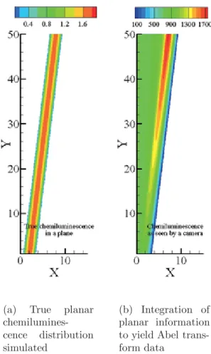
This is the ideal case. This approach allows to check the validity of the developed soft- ware. At first, a simple doughnut like emission is considered. Signal is always positive and negative values arising from those equations are set to zero. In the following, X,Y as well as the chemiluminescence signal will be presented without units.
d0= 2 +Y /50×6
signal= exp(1)−exp((d0−r)2/2) (6) where d0 is the position for which emission is the strongest within a vertical plane, Y is the streamwise position. In the following, only half of the domain is considered as axi-symmetry exists. To create the image of the chemiluminescence as seen by a virtual camera, the entire domain is simulated (X,Y,Z) and the intensity of pixels are summed up along rows (Z) to give the intensity as seen by each pixel (X,Y). The procedure is repeated for a different height (Y). A typical true planar distribution of the simulated signal is represented in Figure 5(a) with its three dimensional integrated
result shown in Figure 5(b). One can for instance observe that even though the peak signal is constant in the planar profile, values close to the exit are much lower than those measured further downstream. This is an important fact to understand and keep in mind when analyzing measurements done with chemiluminescence.
(a) True planar chemilumines- cence distribution simulated
(b) Integration of planar information to yield Abel trans- form data
Figure 5: Presentation of test case 1 for Abel inverse transform without noise and without absorption.
To better compare the effectiveness of the inverse Abel transform, two profiles are taken, one at Y=10 (Figure 6(a)) and the other one at Y=40 (Figure 6(b)). One can clearly notice that the peak of emission is well retrieved when applying inverse Abel transform and that the thickness of the actual ”flame front” is also recovered. Of course, this case being for a simulation without noise is an ideal case.
Some flames may have a double structure (as reported in [13]). It may also be the case of a pilot supported combustor, with an inner flame coming from pilot combustion and the outer flame from the main combustion. Therefore, it is important to verify that Abel inversion is able to find such a double peak and to see also the typical uncertainties associated with those cases. Together with previous equations, a new emission is given by
signal= exp(1)−exp((d0/2−r)2/2) (7)
X
Planarchemiluminescence 3Dchemiluminescence
0 2 4 6 8 10
-0.5 0 0.5 1 1.5 2 2.5
-250 0 250 500 750 1000 1250
True 2D chemiluminescence Retrieved planar distribution 3D Chemiluminescence
(a) Profile at Y=10
X
Planarchemiluminescence 3Dchemiluminescence
0 2 4 6 8 10
-0.5 0 0.5 1 1.5 2 2.5
-250 0 250 500 750 1000 1250 1500 1750
True 2D chemiluminescence Retrieved planar distribution 3D Chemiluminescence
(b) Profile at Y=40
Figure 6: Comparisons between true profile and results obtained through inverse Abel trans- form for test case 1
Typical planar images are given in Figure 7(a) for true distribution and in Figure 7(b) for integrated results. The integrated results show a stronger signal in the inner side of the flame, even though the signal was equivalent for the inner and outer flame.
This emphasizes the fact that analyzing integrated results tend to provide wrong views of actual phenomena.
In the case of a double structure, the intensity retrieved for a height Y of 10 and of 40 is shown in Figure 8(a) and 8(b) respectively. One can see that the outer part of the signal is properly retrieved. The peak coincides with the imposed peak. However, some discrepancies appear as far as inner peak is concerned. Results are also more noisy.
Therefore, in case of pilot supported flame, one has to be careful with the findings of the inner flame and treat them with a greater care than those of simple flame or than the outer flame in the double-structure case. However, the intensity of both inner and outer are correctly reproduced, which allows a possible interpretation on the dynamics inside the combustor.
4.3 Effects of absorption
To see the effects that absorption of chemiluminescence may have on the Abel inversion, different absorption laws have been tested. Absorption may come from several reason, the biggest being some liquid jets like in cryogenic flames. The first law is to say that radiation may be blocked by liquid jets. A simple law of absorption is used:
absorption∝(1− X
DLOx) (8)
In the above equation, DLOx corresponds to the radius below which all radiation is considered as blocked. To model the signal as seen by a camera, one can not use the Abel transform. Instead, a complete computation of the intensity in 3D is done and the projection is done by considering absorption for the region behind the liquid jet.
The radius of the jet is DLOx = 3.2 for Y=10 and DLOx = 5.6 for Y=30. Results of
(a) True planar chemiluminescence distribution
(b) Integration of planar information to yield Abel trans- form data
Figure 7: Presentation of test case 2 for Abel inverse transform for a double flame, without noise and without absorption
X
Planarchemiluminescence 3Dchemiluminescence
0 2 4 6 8 10
0 0.5 1 1.5 2
0 250 500 750 1000 1250 1500 1750 2000
True 2D chemiluminescence Retrieved planar distribution 3D Chemiluminescence
Y = 10
(a) Profile at Y=10
X
Planarchemiluminescence 3Dchemiluminescence
0 2 4 6 8 10
0 0.5 1 1.5 2 2.5
0 400 800 1200 1600 2000
True 2D chemiluminescence Retrieved planar distribution 3D Chemiluminescence
Y = 40
(b) Profile at Y=40
Figure 8: Comparisons between true profile and results obtained through inverse Abel trans- form for test case 2
the chemiluminescence profile at Y=10 and Y=30 are displayed in Figure 9. One can see that the inverse Abel transform becomes negative for radius smaller than 3.15 for Y=10 and smaller than 5.5. Those limits correspond indeed to the outer part of the liquid column.
X
Planarchemiluminescence 3Dchemiluminescence
0 2 4 6 8 10
-1.5 -1 -0.5 0 0.5 1 1.5 2
0 250 500 750 1000 1250 1500 1750
True 2D chemiluminescence Retrieved planar distribution 3D Chemiluminescence Y = 10
(a) Profile at Y=10
X
Planarchemiluminescence 3Dchemiluminescence
0 2 4 6 8 10
-1.5 -1 -0.5 0 0.5 1 1.5 2
0 250 500 750 1000 1250 1500 1750
True 2D chemiluminescence Retrieved planar distribution 3D Chemiluminescence Y = 30
(b) Profile at Y=30
Figure 9: Comparisons between true profile and results obtained through inverse Abel trans- form for test case 3 with linear absorption from an inner liquid jet
Of course, in practice, the detection of negative chemiluminescence signal may not only result from absorption, but also from a non-symmetric pattern or noise. The effects of noise may be lowered by using filtering techniques on the images, like low- pass filters to remove high-frequency noise.
4.4 Effects of lens used
Another important issue when applying inverse Abel algorithm is that the actual rays of lights are not exactly parallel with respect to the imaging plane. To evaluate the differences, simulations are carried using a complete 3D description of the flame coupled to optical geometry to compute the actual emission capture by each different pixel.
The present case will evaluate different distances of the camera from the center of the flame and different camera resolutions, matching the experimental characteristics of the intensified camera that will be used afterwards. However, to avoid complete description of the lenses, spherical lens approximation is used.
Table 2 summarizes the effects of the lens on the angular resolution achieved. Using a lens of 200mm will enable to have a limited field of view (12◦20) and therefore the working distance may be increased. The working distance reported in Table 2 is a rela- tive working distance to capture an object of size 1 (used hereafter for normalization).
One can see that a 50mm lens would require a very small working distance.
The pixels of the camera are considered as being a unique point compared to the distance with respect to the flame, whatever the lens used. The problem simulated is depicted in Figure 10.
The parameters investigated will first be the ratio between the distance from the camera and the centre of the flame to the diameter of the flame. This first parameter
Lens 50mm 105mm 200mm Angle 46◦ 23◦20 12◦20 Distance 2.35 4.84 9.26
Table 2: Angular dispersion as function of lens
Figure 10: Sketch of the Simulation of a true chemiluminescence signal as seen by a camera
will be calleddistance. This parameter depends on the focal length of the lens used and therefore when presenting results, the focal length will be used. All illustration will be done with an axis between 0 and 1, 0 representing the center of the simulated camera and 1 the highest pixel number. Therefore, the represented pixel number will be half of the simulated one, the other half not being displayed due to symmetry. The lines along which integration is performed for the 100th pixel out of 384 is displayed in Figure 11. In this graph, an ideal case would correspond to a vertical line. One can see that a big difference arises for the 50mm case.
This is further illustrated in the profile of the recorded chemiluminescence, the effects of the focal length is represented in Figure 12(a). One can clearly see the differences in the profiles between a lens of 50mm and 105mm. Differences tend to decrease for lenses with focal length higher than 105mm. A distance of 10,000 is also simulated as being the ideal case and therefore is shown as being ∞.
The planar profiles retrieved from those different measurements are shown in Figure 12(b). One can clearly see that a 50mm lens would give a result slightly different from the other cases in both the position of the peak as well as the width of the distribution.
This may have some consequences when analyzing the measurements and therefore, 50mm focal length should not be used when performing inverse Abel transform.
Even though, Abel transform seems straightforward, many effects have to be taken into account to be really able to propose semi-quantitative data from a 3D distribu- tion. The effects on actual configurations on the uncertainties being qualified, one may proceed to the application of this inverse Abel scheme.
X
Z
-1 -0.5 0 0.5 1
-1 -0.5 0 0.5 1
f = 50 mm
f = 105 mm f = 200 mm
64B?2 62?2;02@ 6; 6;A24?.A6<; 96;2 .@ 3B;0A6<; <3 3<0.9 92;4A5 %.F A?.06;4 .@ @22; /F A52 =6E29 <BA <3 =6E29@
< $D@M@I>@N DI NDBI<G N@@I =T OC@ ><H@M<
KDS@GN <N API>ODJI JA AJ><G G@IBOC >JH K<M@? OJ <I D?@<G ><N@
X
Retrievedplanardistribution
0 0.2 0.4 0.6 0.8 1
True profile f = 50 mm f = 105 mm f = 200 mm
= #JHK<MDNJIN =@OR@@I OC@ ?D@M@IO KG<
I<M DIAJMH<ODJI M@OMD@Q@? <N API>ODJI JA AJ><G G@IBOC
64B?2 20A@ <3 92;@ 3<0.9 92;4A5 <; 052:69B:6;2@02;02 =?<92@
5 Combustors
In the following, two different combustor will be alternatively used to show the utility of chemiluminescence in active control loop. Both combustor run with lean premixed methane-air at atmospheric pressure. The main differences reside in the pressure levels achieved for the natural oscillating mode as well as the adiabatic temperature of the flame (equivalence ratio) at which strong oscillations occurred. Both combustors have identical mixing chamber.
5.1 Swirler without recess
The first combustor (see Figure 13) has an overall length of 810mm. The outer and inner diameters of the swirler are respectively 50 and 20mm and is composed of 12 vanes of 30 degree angle. The inlet temperature is set to 500K with an overall mass flow rate of 60 g·s−1. Strong oscillations occur for equivalence ratio laying between 0.65 and 0.85. Typical pressure fluctuations (see Figure 14) are around 0.75 to 1.2 kPa and subsequent frequencies are found around 200Hz. The emission index is measured at two different positions (at the exit of the combustor and 100mm inside the combustor).
Figure 13: First setup used to evaluate chemiluminescence
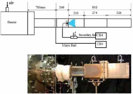
5.2 Swirler with recess
The second combustor (see Figure 15) is run at 700K with a mass flow rate of 78 g·s−1 for the air (or a total flow rate of 1500Nl/min). The overall equivalence ratio studied caries between 0.43 and 0.60, which corresponds to adiabatic temperature between 1660 and 1960K. The first part of the combustor (up to 210mm downstream the swirl) is composed of four quartz to allow complete optical access. The second part (420mm long) consists of water-cooled stainless plate. The chemiluminescence measurements
Equivalence ratio ( - )
Emissionindex(NOx) Pressurefluctuations[kPa]
0.6 0.7 0.8 0.9
0 2 4 6 8 10 12
0 0.2 0.4 0.6 0.8 1 1.2
X = 0mm X = -100 mm rms (kPa)
Results of pressure fluctuations for combustor#1
Figure 14: Characteristics of the combustor#1 in terms of pressure levels and emission index
have been taken in the first section, using either a simple fiber to get complete view of the section or a dual lens system in order to spatially limit the zone of interest. Both approaches provide slightly different data and they are examined in the next sections.
The pressure sensor (Kulite Semiconductor Products, Inc., Model XTL-190-15G, lo- cated 10mm from the exit of the swirl) as well as the time series chemiluminescence are acquired simultaneously through a multi-channel data acquisition system (ONO SOKKI, DS-200, Graduo). Typical sampling frequency is 25.6kHz for each channel.
The pilot injection is referred as percentage versus the total fuel injected. If one refers to the main mixture’s injection, this would lead to a value of 0.2%.
Figure 15: Sketch of the combustor #2
The typical pressure observed for over different equivalence ratio of (fromφ= 0.43 to 0.65 is displayed in Figure 16. The subsequent emission index of both NOx and CO is displayed in Figure 17. One can see that typical low emissions can be achieved for
overall equivalence ratio around 0.50 and that this value corresponds to the peak of pressures.
Figure 16: Pressure spectra for equivalence ratio ranging betweenφ= 0.43 and 0.65
This is therefore considered as a setup typically representing the main problems in actual gas turbines: running in stoichiometry close to the blow-off to reduced emission may induce spurious pressure oscillations. To fully understand the nature of those oscillations and propose strategies to control them, chemiluminescence is used through imaging systems, by spectrally resolved measurements to give some hints about chemical reactions and by temporally resolved to show coherent behavior between pressure and chemiluminescence emission.
Adiabatic flame temperature [K]
EINOx[g/kg] EICO[g/kg]
1700 1750 1800 1850 1900 1950 0
0.1 0.2 0.3 0.4 0.5 0.6 0.7
0 0.5 1 1.5 2 EI NOx
EI CO
T=700K, V=90m/s, vane angle=45deg, no secondary injection x: 50mm upstream from chamber exit. Averaged over 7 points.
(y,z)=(0,0),(5,5),(10,10),(15,15),(20,20),(25,25),(30,30).
Figure 17: Emission index of NOx and CO for equivalence ratio ranging between φ = 0.43 and 0.65
6 Results with imaging approach
For active control, the imaging techniques may lack of frequency response. Some alternatives may be found in linear photodiode arrays, like proposed in [14] to have both a temporal and spatial resolution. In the present case, standard intensified cameras are used. The objectives is to provide a spatial description of the flame dynamics, through the computations of a Rayleigh index map to enhance regions for which the coupling between heat release and pressure oscillations is strong.
Oscillating combustion is characterized by peak pressures that usually are easily measured. The frequency of the phenomena being relatively constant, the triggering of external measurements like phase-locked chemiluminescence images can be done. In the present part, the results obtained by triggering the chemiluminescence acquisition as function of the pressure signal are presented. The reference for pressure signal will always be taken at the point for which the signal is zero with a positive slope.
6.1 Visualization of flame structure
To better understand the mechanisms of oscillating combustion, phase-locked images of chemiluminescent emissions in case of oscillations are recorded. The pressure trans- ducer is located at X = 20mm and Y = 0mm. The global chemiluminescence of OH∗ is recorded as function of the phase delay with respect to the pressure signal. For that purpose, an ICCD (Princeton Instruments 576G/1) is used to capture the images of OH∗, with an UV-Nikkor 105mm/f4.5 lens. Its resolution is 576 by 384 pixels and typ- ical measured area were 75mm×50mm, which gives a magnification 0.13 mm2/pixel.
It is used in gate mode with an exposure of 40 μs and a f-number of 4.5. Typically 80 images are recorded at each phase angle (20 points in case of oscillating flames, 10 points otherwise). The phase is determined with respect to the zero-crossing event in the filtered pressure signal with a positive slope. The filter had a bandwidth of 10Hz centered around the desired frequency. An illustration of the different phases is given in Figure 18 as well as a typical pressure signal within the combustor.
The flow comes from left to right (see Figure 19-20) and the bulk velocity of 12m·s−1 for an inlet temperature of 500K, the length of the combustor being 810mm; the typical frequencies are around 220Hz. The overall equivalence ratio for the case in Figure 20 is 0.73 (see Table 3 for full details) for a fully premixed case. Background is removed from all images and levels lower than 1% of the maximum are removed also for clarity reason. The images correspond to volume integration as no Abel transform is applied.
One can notice an influence on the flame shape as a function of pressure phase.
Case φ Pilot[%] Frequency [Hz] Pressure [kPa]
Figure 19 0.73 0 220 1.83
Figure 20 0.87 10 245 1.83
Table 3: Experimental conditions
For the case of φ= 0.73 and a phase delay of 10◦, the flame front close to the exit seems to be deformed by a vortex-like structure coming from the inside of supplying mixture (height Y between 10 and 25mm). For a phase of 45◦, this behavior is em- phasized with the same structure being detected. For a phase of 90◦, which represents
Figure 18: Raw and filtered pressure signal. Band-pass filter centered on the desired fre- quency is used.
Figure 19: Phase-locked visualization of the unsteady process for premixed oscillating flame φ= 0.73
Figure 20: Phase-locked visualization of the unsteady process for partially premixed flame φ = 0.87
the time where the pressure is at its maximum for a position of X=20mm along the centerline, the overall chemiluminescent emission increases. This increase is also seen for a phase delay of 125◦, but at the position of the pressure probe (which is the line over which the chemiluminescent lens is integrated), one can notice that the emission diminishes. At this time, the outer part of the flame seems to be deformed whereas the central parts (for radial positions lower than 20mm) have a flat profile. For delays between 125◦ and 205◦, one can notice that the boundaries as seen by the chemilumi- nescence seems to be moving with the mean flow, as typically low levels only can be found for temporal positions around 205◦ and 245◦. The fact that no signal appears for a delay of 285◦ does not mean that the flame is completely lifted up or blown out, simply that the levels may be very small compared to background emission. What is more surprising are the results for delays after 300◦, where a flame front is seen close to the exit of the swirler. It would have been more logical to see a flame front coming from the right side of the combustor (as for instance explained in [15]). Afterwards, this initial flame front develops and a vortex-like structure can be detected, as already mentioned for initial delays.
Somehow similar results can be found in case of secondary injection leading also to oscillating combustion (see Figure 20). The premixed remains unchanged but 10% of methane compared to the previous mixture is added and injected through small holes (1.4mm), placed inside the combustor. The overall equivalence ratio is in this case 0.87. Therefore, the overall chemiluminescence emission is higher for this case than the previous one. The secondary fuel is injected at 245Hz, with an opening time of 1.6ms and a phase delay of 190◦compared to the pressure signal.The same mechanisms are present, even though the flame is not vanishing out of the measurement region. This may comes from higher equivalence ratio (hence higher signal to noise ratio). As can be seen for a phase delay of 250◦, the central part exhibit chemiluminescent emission.
This is an effect of secondary injection. This case leading to oscillations was a case for which the time delay between secondary injection and pressure was 2ms. Having a time lag of 72ms, this makes 74ms, resulting in a true phase shift of 160◦, with an opening of 1.6ms, representing 65◦.
6.2 Planar Rayleigh Index measurements
With the previous results, it is relatively hard to understand the true nature of the dynamics within the combustor. For a better image, one has to retrieve a planar information, using inverse Abel transform (see section 4). The present geometry having a square section, caution has to be made when dealing with results obtained close to the wall. In those regions, the axi-symmetry assuption is not valid. As stated in section 4, for practical cases, filters have first to be used to reduce the noise. A typical noise filtering is performed using low-pass filters with different kernel sizes. The kernel size is expressed in pixels and varies from 10 to 30. The filter is based on a pixel-wise adaptive Wiener method based on statistics estimated from a local neighborhood of each pixel. The difference can already be seen in the profile to treat. A comparison between no filter, a filter of 10 and 30 pixels is presented in Figure 21. One can clearly see that the raw chemiluminescence signal contains high-frequency noise. This noise will lead to erroneous results as far as inverse Abel transform is concerned. On the other hand, a filter with a 30 kernel seems to damp too much the low-frequency changes observed in the signal. Those low-frequencies phenomena may come from combustion
and therefore shall be kept.
Radial position (mm)
Emission(A.U.)
0 10 20 30 40 50
0 50 100 150 200 250
Raw signal 10 Kernel 30 Kernel
Figure 21: Effects of kernel size on raw signal
Therefore, for the following data, only a kernel size of 10 pixels by 10 pixels will be used to compute the planar chemiluminescence emission.
A typical difference of integrated results (Figure 22(a)) and Abel inverted result (Figure 22(b)) is presented.
(a) Raw chemiluminescence image (b) Subsequent Abel inverted image
Figure 22: Phase delay of 0◦ for combustor #2 and φ= 0.50: oscillating frequency 250Hz
This example clearly illustrates the importance of using Abel inverted images. One can see that the zone for which intense emission is detected is much smaller than in the raw image and closer to the exit of the swirler.
Another important parameter prior to compute a Rayleigh map is to estimate the pressure levels. The exact definition of the Rayleigh index is
! "
! " ! "
RCD>C M@LPDM@N OC@ FIJRG@?B@ JA =JOC P>OP<ODIB KM@NNPM@ <I? P>OP<ODIB C@<O M@G@<N@ DI <GG KJDION JA OC@ >JH=PNOJM )I KM<>OD>@ JI@ <NNPH@N < NK<OD<GGT PIDAJMH KM@NNPM@ @G? DI OC@ DH<BDIB <M@< AJM @<>C KC<N@ 3CDN CTKJOC@NDN ><I =@ EPNOD@?
=T OC@ A<>O OC<O OC@ KM@N@IO DINO<=DGDOD@N <M@ >JHDIB AMJH < GJIBDOP?DI<G HJ?@ LP<M O@M R<Q@G@IBOC <I? OC<O OC@ KM@NNPM@ @G?N JN>DGG<O@ DI KC<N@ &PMOC@MHJM@ M@NPGON KM@N@IO@? DI :; >G@<MGT NCJR@? OC<O OCDN CTKJOC@NDN ><I =@ H<?@ !N C@<O M@G@<N@
><I IJO =@ H@<NPM@? JI@ C<N OJ <NNPH@ OC<O C@<O M@G@<N@ <I? >C@HDGPHDI@N>@I>@ <M@
KMJKJMODJI<G OJ @<>C JOC@M 3C@ @S<>O G@Q@G JA OC@ KM@NNPM@ NDBI<G H<T IJO =@ J=O<DI@?
<I? OC@M@AJM@ JI@ H<T M<OC@M ?@O@MHDI@ OC@ ?@BM@@ JA >JPKGDIB =@OR@@I KM@NNPM@ <I?
>C@HDGPHDI@N>@I>@ M<OC@M OC<I OC@ Q<GP@ JA OC@ KMJ?P>O
! "
OH ! "
3C@M@AJM@ DI KM<>OD>@ OC@ >JPKGDIB DN ?@O@MHDI@? <O @<>C KJDIO <I? ?DQD?@? =T OC@
Q<GP@ OC<O RJPG? M@NPGO AMJH < K@MA@>O >JPKGDIB NDIPNJD?<G >C<IB@N DI KC<N@ 3CDN Q<GP@ DN >JIO<DI@? =@OR@@I KC<N@ JA <I? K@MA@>O KC<N@ H<O>CDIB <I? DN
><GG@? >JMM@G<ODJI =@OR@@I KM@NNPM@ <I? >C@HDGPHDI@N>@I>@
< 2K<OD<G >JMM@G<ODJI H<K
Phase (o)
Chemiluminescence(A.U.)
0 90 180 270 360
0 5 10 15 20 25
X = 20 and Y = 10 X = 20 and Y = 20 X = 20 and Y = 40 X = 40 and Y = 20
= &GP>OP<ODJIN JA >C@HDGPHDI@N>@I>@ <O AJPM ?D@M@IO KJDIO AJM
64B?2 <??29.A6<; /2AD22; =?2@@B?2052:69B:6;2@02;02 6; 0<:/B@A<? 3<?
<@0699.A6;4 3?2>B2;0F G
3C@ M@NPGON AJM I<OPM<G JN>DGG<ODJIN DI >JH=PNOJM <M@ NCJRI DI &DBPM@ <
/I@ ><I N@@ H<DIGT ORJ ?D@M@IO M@BDJIN C<QDIB < >JMM@G<ODJI >GJN@ OJ PIDOT 3C@ MNO M@BDJI >JMM@NKJI?N OJ OC@ @SDO JA OC@ DI>JHDIB HDSOPM@ 3C@ JOC@M JI@ DN GDIF@? RDOC OC@
M@>DM>PG<ODJI 3C@ <H@ KM@N@ION < OM<INDODJI JA NOMP>OPM@ AMJH OC@ DIQ@MO@?>JID><G
<H@ OJ OC@ MDH <H@ J>>PMM@? =@OR@@I ! NOMJIB >JPKGDIB DI OC@ MNO
region may come from upstream modifications of the incoming mixture due to pressure oscillations. In fact, it has been shown [17] that the equivalence ratio is modified due to the strong pressure oscillations and that for an overall mean equivalence ratio of 0.50, the actual equivalence ratio varies between 0.48 and 0.52, with a minimum for a phase of 135◦ and a maximum for 225◦.
To illustrate further this tendency, the fluctuations of chemiluminescence at four different points within the previous image are shown in Figure 23(b). One can clearly see that the fluctuations of chemiluminescence at X=20,Y=40 are shifted with respect to other points. As shown in the spatially resolved map, this point is not strongly influenced by thermo-acoustics oscillations as correlation is close to zero.
This section showed the different data obtained through imaging techniques. The results clearly emphasized the importance to localize the regions of strong coupling be- tween chemiluminescence and pressure to provide directions as far as active control is concerned. Next developments will deal with spectrally resolved data.
!-/&.- 1%.$ -*!.,&&3 ,!-)&0! $!'%&/'%
(!-!(!
!.%&! (&3-%- )" -*!.,
2K@>OM<G <I<GTNDN JA OC@ <H@ J@MN Q@MT @<NT =PO CJR@Q@M Q@MT AMPDOAPG DIAJMH<ODJI JI OC@ >JH=PNODJI HJ?@ )O DN FIJRI OC<O G@<I KM@HDS@? >JH=PNODJI RDGG H<DIGT >M@<O@
/( M<?D><GN <I? OC<O M<?D><GN NP>C <N #( <I? #2 RDGG =@ Q@MT GDHDO@? 3J DGGPNOM<O@
OC@ G@<I KM@HDS@? =@C<QDJM H@<I NK@>OM< <M@ O<F@I RDOCDI JN>DGG<ODIB >JH=PNODJI 3C@ NK@>OMJH@O@M PN@? DN OC@ -2 AMJH /MD@G >JPKG@? OJ <I )##$ AMJH !I?JM O@>CIJGJBT $(& KDS@GN 3C@ )##$ DN PN@? DI B<O@ HJ?@ RDOC <I
@SKJNPM@ JA N RCD>C >JMM@NKJI?N OJ Q<GP@N GJR@M OC<I AJM JN>DGG<ODIB >JH=PNODJI DIO@IND><ODJI JA <I? < NGDO JA H &PGG Q@MOD><G =DIIDIB DN K@MAJMH@? <I?
<>>PHPG<ODJI JQ@M N<HKG@N DN O<F@I AJM @<>C KJDIO &JM OCJN@ H@<NPM@H@ION <
N@MD@N JA ORJ G@IN@N R<N PN@? 3C@ G@IN R<N KG<>@? K@MK@I?D>PG<M OJ OC@ >JH=PNOJM RDOC < AJ><G KJDIO DI OC@ >@IO@M JA OC@ >JH=PNOJM HH DI OC@ NOM@<HRDN@ ?DM@>ODJI
<N R@GG <N DI OC@ OM<INQ@MN@ ?DM@>ODJI AMJH OC@ >@IO@M 3C@ A<>O OC<O H<DIGT /( DN
< 3TKD><G NK@>OM< AJM G@<I KM@HDS@? <H@
AJM
= 3TKD><G NK@>OM< RC@I PNDIB <>ODQ@ >JI
OMJG AJM
64B?2 &=20A?.99F ?2@<9C21 052:69B:6;2@02;02 D6A5<BA .;1 D6A5 @20<;1.?F 6;720A6<; 3<?
0<;A?<9921 0.@2@
QDND=G@ AJM G@<I KM@HDS@? >JH=PNODJI DN K@MA@>OGT NCJRI DI &DBPM@ < AJM RCD>C OC@
JQ@M<GG @LPDQ<G@I>@ M<ODJ O<F@I R<N S@? <O RDOCJPO <IT KDGJO 3C@ <=NJGPO@ Q<GP@
JA OC@ DIO@INDOT JA OC@ NDBI<G DN IJO O<F@I DIOJ <>>JPIO <I? OC@M@AJM@ JIGT < M@G<ODQ@
DIO@INDOT DN NCJRI JI OC@ G@AO <SDN /I@ ><I IJOD>@ OC@ /( K@<F <MJPI? IH <I?
JI@ H<T ?DNODIBPDNC <MJPI? IH < N@>JI?<MT K@<F DI?P>@? =T #( M<?D><GN @Q@I OCJPBC DON Q<GP@ <=JQ@ OC@ =<>FBMJPI? DN IJO Q@MT DIO@IN@ #2 M<?D><GN <M@ IJO QDND=G@
AJM NP>C G@<I >JI?DODJIN /I OC@ JOC@M C<I? GJJFDIB <O >JIOMJGG@? ><N@N OCMJPBC <
N@>JI?<MT DIE@>ODJI JA AP@G JI@ ><I IJOD>@ OC@ <KK@<M<I>@ JA NOMJIB #( IH <I?
IH <I? #2 @HDNNDJI <MJPI? <I? IH <N NCJRI DI &DBPM@ = 3CDN DN
< >G@<M DI?D><ODJI JA OC@ ?DPNDJI KMJ>@NN DI?P>@? =T OC@ DIE@>ODJI JA OC@ KDGJO 3CDN
may has, as a consequence, strong effects on nitrous oxide emissions and therefore, for completing active control schemes, it is important to check the possible increase in NOx levels induced by this diffusion flame.
For active combustion, one may look more for temporal information to see changes within the combustor. Therefore, the next part presents typical temporal results ob- tained.
7.2 Determination of operating point control
To have a minimum of pollutant emission as well as a safe margin compared to blow off or oscillating combustion, the exact equivalence ratio should be known at any time.
However, in gas turbines, the exact amount of air supplied is not precisely known and variations in the fuel properties may also affect the actual stoichiometry. Therefore, it is of practical importance to have a real time monitoring of this quantity. However, gas turbines are harsh environment and therefore, non-intrusive techniques are preferable.
Some studies have shown that it may be possible to record incoming equivalence ratio using absorption techniques ([18]). However, again problems may come from long terms use of laser source and the influence of oscillations may not be negligible. Therefore, chemiluminescence was chosen but whereas many studies reported before ([10], [19], [20]) used spectrometer (low time resolution) the present sensing device can have higher temporal measurements.
Chemiluminescence is measured through a system of lens with a focal length of 300mm. The light exiting the lens is sent, through an optic fiber to a specbox (Hama- matsu, Inc.). This divides afterwards, through a series of band-pass filter and mirrors to four different photo-multipliers. The optical properties of each band-pass filters as well as the radical measured are shown in Table 1. It is worth noting that the two last wavelengths are representing the background emission in lean premixed flames, as it has been shown that C∗2 radicals can hardly be detected for typical stoichiometry below 0.90 [8]. The measurement is resulting from the integration over a volume and therefore no fine spatial resolution can be obtained. It has been shown in [21] that monitoring the ratio of (OH∗-background) / (CH∗- background) lead to an indication of the actual stoichiometry. To validate the presented approach (use of 3 different PMT rather than one spectrometer for a considerable gain in the frequency domain), measurements are also performed inside the target combustor. It is a swirl-type stabilized flame, having 12 vanes of 30◦ of angle each. The dimensions of the combustor are 100×100mm for the section and a total length of 210mm, extensible to 810mm to change the acoustic frequencies. An important feature is the presence of secondary injection orifices that may be used for active control strategies. The calibration is done without injecting the secondary fuel, considering only premixed methane-air flames. The location of the lens is at 20mm from the exit of the swirl, along the centerline of the combustor. Typical variable are inlet temperature and inlet velocity. The measured ratio is obtained using three different photo-multipliers, each having different voltage. The voltage is actually corrected to obtain a more uniform relation. Calibration was performed for a velocity of 30m·s−1, pre heated at 700K. One can notice on Figure 25(a) that the initial slope (for equivalence ratio (E.R.) below 0.5) is very steep, meaning that small changes in the stoichiometry leads to strong changes in the ratio between OH∗ and CH∗. The background is removed on both signals (using PM3, emission between 471 and 475 nm). The results presented here are mean results obtained over 10s.
< #C@HDGPHDI@N>@IO M<ODJN DI ?@HJINOM<
ODJI >JH=PNOJM
= 3DH@ N@MD@N @Q<GP<ODJI JA NOJD>CDJH@OMT
64B?2 2A2?:6;.A6<; <3 A52 <=2?.A6;4 =<6;A 0<;A?<9 B@6;4 ?.A6< #
3CDN DN Q@MT DIO@M@NODIB <N OC@ G@<I =GJRJPO GDHDO GD@N RDOCDI <I? ?@K@I?DIB JI OC@ Q@GJ>DOT >CJN@I /I@ ><I IJOD>@ OC<O OC@ G@IBOC JA OC@ >JH=PNOJM <@>ODIB NOMJIBGT OC@ DII@M <>JPNOD>N C<N IJ DIP@I>@ JI OC@ M<ODJ 3C@ <>OP<G M<ODJ DN IJI HJIJOJID> <N <GNJ J=O<DI@? OCMJPBC OC@ IPH@MD><G NDHPG<ODJIN JA OC@ >C@HDGPHDI@N
>@I>@ @HDNNDJI N@@ 2@>ODJI 3C@ Q<GP@ AJM RCD>C OC@ @HDNNDJI M<ODJ DN H<SDHPH NGDBCOGT ?D@MN =@OR@@I @SK@MDH@IO<G <I? IPH@MD><G M@NPGON <N NCJRI KM@QDJPNGT DI 2@> 3C@ ?D@M@I>@ H<T >JH@ AMJH PI>@MO<DIOD@N DI OC@ H@<
NPM@H@ION ?P@ OJ M@G<ODQ@GT GJR @HDNNDJI G@Q@GN JM AMJH OC@ >JINO<IO PN@? OJ >JHKPO@
@HDNNDJI (JR@Q@M DI OC@ M@BDJI RC@M@ =GJRJPO H<T J>>PM G@NN OC<I OC@
NC<K@ DN HJIJOJID> G@<?DIB OJ IJI<H=DBPJPN M@NPGON
!IJOC@M KJDIO >JINDNON DI ?@O@MHDIDIB OC@ OTKD><G O@HKJM<G M@NKJIN@ <I? <>>PM<>T JA OCDN H@<NPM@H@IO 3C@ =PGF Q@GJ>DOT DN N@O OJ HN1 KM@C@<O@? <O + 3C@
Q<GP@ JA OC@ =GJRJPO DN AJM OCDN ><N@ 3CDN DN DGGPNOM<O@? DI &DBPM@ = RC@M@ ORJ N<HKGDIB M<O@N <M@ >JIND?@M@? (U <I? (U 3C@ DHKJN@? @LPDQ<G@I>@
M<ODJ DN M@NK@>ODQ@GT <I? /I@ ><I IJOD>@ OC<O OC@ H@<NPM@? @LPDQ<G@I>@ M<ODJ DIA@MM@? AMJH H@<NPM@? >C@HDGPHDI@N>@I>@ M<ODJ DN DI BJJ? <>>JM?<I>@ RDOC M@NK@>O OJ OC@ DHKJN@? JI@ -@<NPMDIB OC@ OTKD><G ?@QD<ODJIN <N API>ODJI JA OC@ N<HKGDIB AM@LP@I>T BDQ@N <I D?@< JA OC@ PI>@MO<DIOD@N 3C@ M@NPGON <M@ ?DNKG<T@? DI &DBPM@
RC@M@ RDI?JRN AMJH OJ N AM@LP@I>D@N =@OR@@I <I? (U <M@ >JIND?@M@? AJM OCM@@ ?D@M@IO NOJD>CDJH@OMT /I@ ><I N@@ OC<O O<FDIB RDI?JRN JA N OJ H@<NPM@ OC@
@LPDQ<G@I>@ M<ODJ OCMJPBC >C@HDGPHDI@N>@I>@ M<ODJ BDQ@N M<DN@ OJ OTKD><G PI>@MO<DIOD@N JA OC@ JM?@M JA OJ RCD>C H<T M@KM@N@IO 3C@ CDBC@NO @MMJMN <M@ AJPI? AJM
@LPDQ<G@I>@ M<ODJ <MJPI? =@><PN@ DO C<N =@@I NCJRI OC<O OC@ /(#( DN Q@MT N@INDODQ@ DI OCDN M@BDJI 4NDIB GJR@M N<HKGDIB AM@LP@I>T (U JM (U @I<=G@N OJ M@?P>@ ?M<NOD><GGT OC@ PI>@MO<DIOD@N OJ G@Q@GN =@GJR AJM OC@ ?D@M@IO ><N@N NCJRI C@M@
3C@ PI>@MO<DIOT DN >JHKPO@? <N =@DIB OC@ H@<NPM@H@ION JA OC@ M@G<ODQ@ P>OP<ODJIN
<MJPI? OC@ <Q@M<B@? Q<GP@ JM MJJO H@<I NLP<M@ 3CDN DN EPNOD@? <N NO@<?T HDSOPM@ DN PN@? AJM OCJN@ O@NON
Frequency of acquisition (Hz)
Relativefluctuations(%)
0 2 4 6 8 10 12
0 0.5 1 1.5 2 2.5 3 3.5 4
φ= 0.40 φ= 0.45 φ= 0.50
Figure 26: Typical uncertainties for lean premixed flames as function of acquisition frequency
In this section, it has been shown that taking the ratio of chemiluminescent species can yield the information concerning the burning equivalence ratio. This information may be used for low frequency (of the order of a few Hertz) loop control of the operating point. The main difference with previously published paper is that high frequency acqui- sition is also possible using this probe and the next section deals with this subsequent advantage compared to spectrometer with lower temporal possibilities.
8 Results with temporally resolved techniques
8.1 Simultaneous measurements of chemiluminescence-pressure for instability characterization
8.1.1 Time series Rayleigh
For active control strategies, it is very important to have sensors that can give in a very short time the appearance of self-sustained oscillations. Pressure signals is of course very efficient for this target, but the increase of pressure fluctuations are the results of the oscillations, not the cause. As known, it is the fact that heat release and pressure fluctuations are in phase that will provide energy to the oscillations, hence re-enforcing them and increasing the levels of pressure, which will in turn increase the levels of energy. Therefore, it seems more appropriate to try to measure the concordance of heat release rate versus pressure fluctuations with a good temporal resolution. The true Rayleigh index definition is the integral over one cycle and for the complete volume of pressure fluctuations times heat release fluctuations. This term is not easily obtained experimentally. Therefore, a slightly different expression is used in the following of this article (see equation 9 and 10).
Computing a mean Rayleigh index (sum of pressure fluctuations times heat release fluctuations over 1 second along the volume of the lens integration), one can see a strong relation between this mean value and the mean pressure fluctuation levels inside the combustor, as depicted by the graph represented in Figure 27(a).
For clarity reason, the logarithmic value (base 10) of the Rayleigh index is plotted on