In this paper we consider a numerical scheme for the following initial-boundary value problem:

A stable finite difference method for a Cahn-Hilliard type equation with long-range interaction

Hikaru M

, Ken-Ichi N

1Graduate School of Natural Science and Technology, Kanazawa University Kakuma, Kanazawa, 920-1192, Japan

Email : [email protected]

2Institute of Science and Engineering, Kanazawa University Kakuma, Kanazawa, 920-1192, Japan

Email : [email protected]

(Received December 20, 2013 and accepted in revised form January 29, 2014)

Abstract We propose a stable numerical scheme for a Cahn-Hilliard type equation with long-range interaction describing the micro-phase separation of diblock copolymer melts.

The scheme is designed by using the discrete variational derivative method, one of structure preserving numerical methods. The derivation of the discrete variational derivative of a dis- cretized energy functional is simplified by using a suitable discreteL²space and fractional powers of a discrete approximation of the Laplace operator. The proposed scheme has the same characteristic properties, mass conservation and energy dissipation, as the original equation does. We also discuss the stability and unique solvability of the scheme.

Mathematics Subject Classification (2010) : Primary 65M06; Secondary 35K35 Keywords. Cahn-Hilliard type equation, nonlocal free energy, discrete variational deriva- tive method, conservative numerical schemes

1 Introduction

In this paper we consider a numerical scheme for the following initial-boundary value problem:

∂

u

∂

t =

−ε

+ W

( u )

−

u − u ), x ∈

t > 0 , (1.1)

∂

u

∂ ν

=

∂ ν

= 0 , x ∈

t > 0 , (1.2)

u ( 0 , x ) = u

( x ), x ∈

(1.3)

where

is a rectangular domain in

,

is the outward unit normal to

, W ( u ) =

1

4

( u

− 1 )

is a double-well potential with equal well-depth and

,

are positive con-

stants.

Problem (1.1)–(1.3) arises in a model of micro-phase separation of diblock copoly- mers where subchains of two different type of monomers are chemically bonded. Repul- sive forces between different monomers induce phase separation. However, macroscopic phase separation does not occur because of the chemical bond and hence microscopic patterns may appear. Ohta and Kawasaki [12] proposed a phenomenological model for the copolymer configuration based on the Landau-type free energy functional incorpo- rated with a Coulomb-type long-range effect. Nishiura and Ohnishi [10] reformulated the energy functional in the following form:

J ( u ) =

Ω

G ( u ,∇u ) dx , (1.4)

G ( u ,∇u ) =

2 |∇u |

+ W ( u ) +

2

(−ΔN

)

( u − u )

, (1.5) where u is a rescaled ratio of the densities of two monomers,

> 0 is a small param- eter depending on the size and mobility of monomers, W ( u ) is a double-well potential with global minima at u = ± 1,

> 0 is a parameter related to the polymerization in- dex, (−Δ

)

is a fractional power of the Laplace operator in

under the zero-flux boundary conditions and

u = 1

|Ω|

Ω

u dx ∈ [− 1 , 1 ]

is the average of the rescaled density ratio. The third term of the energy functional de- scribes nonlocal interactions which prevent copolymers forming large blocks of mono- mers. Indeed, the term is computed by using the Green’s function

x , y ) of −Δ under the zero-flux boundary conditions in the following way:

σ

2

Ω

(−ΔN

)

( u − u )

dx =

2

Ω

|∇v |

dx , where

v(x) =

ΩΓ(x,

y)(u(y) − u)dy.

Due to the compactness of (−Δ

)

, the third term prefers rapid oscillation of u around u [10].

In order to build a dynamical model for diblock copolymers, we consider a mass- conserved gradient flow of the energy functional with respect to the H

-norm. The resulting equation is

∂

u

∂

t =

J

δ

u , (1.6)

where

J /δ u is the (first) functional derivative of J given by

J

δ

u = −ε

+ W

( u ) +

(−Δ

)

( u − u ). (1.7)

Thus we obtain equation (1.1). When

= 0, equation (1.1) reduces to the well-known Cahn-Hilliard equation, a model of macro-phase separation in binary alloys [2].

From the above derivation we easily see that problem (1.1)–(1.3) has mass conserva- tion and energy dissipation properties as follows:

d dt

Ω

u dx =

ΩΔδ

J

u dx =

∂Ω

∂

∂ ν δ

J

δ

u dS = 0 , d

dt J ( u ) =

Ω

δ

J

u

∂

u

∂t

dx = −

Ω

∇ δ

J

δ

u

²

dx ≤ 0 .

Here we used the fact that the normal derivative of each term of

J /δ u vanishes on

due to the boundary conditions (1.2).

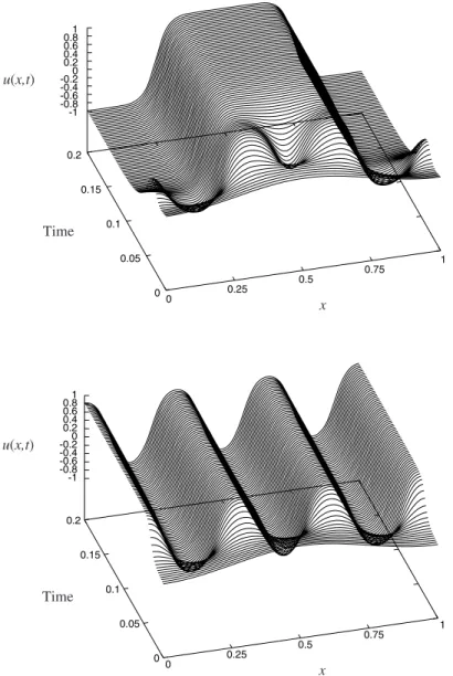
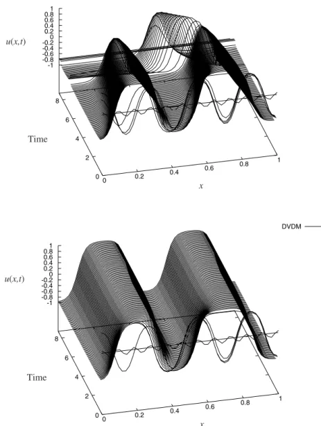
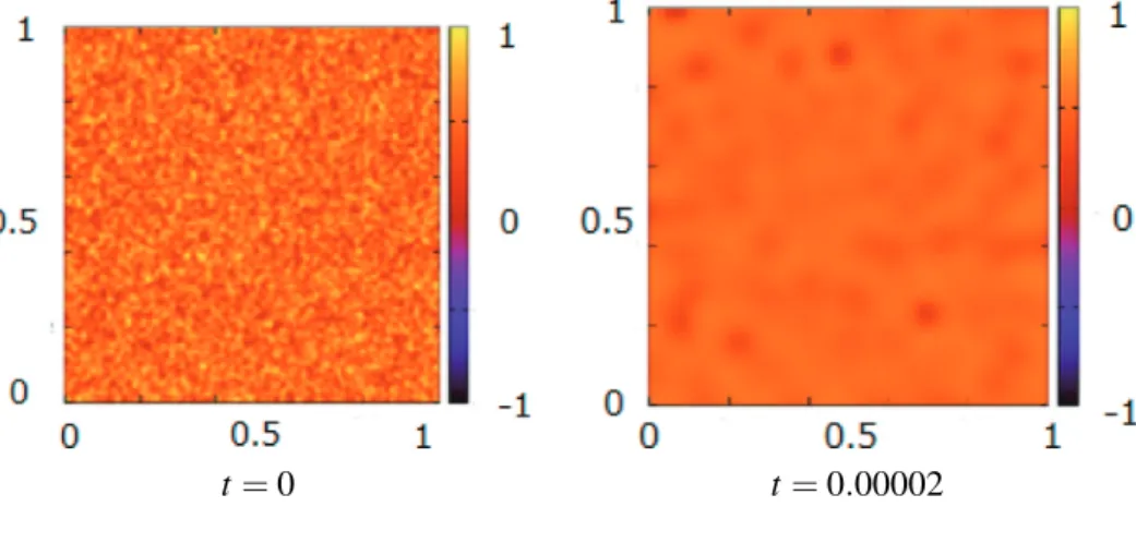
It is experimentally and numerically known that the final asymptotic states in the evo- lution of the copolymer configuration are periodic patterns such as lamellar, cylindrical, spherical and gyroid structures [1, 9]. However, it is not easy to solve numerically the Cahn-Hilliard-type equation (1.1). One reason is that the right-hand side of (1.1) includes the term

( u ) = ( 3u

− 1 )Δu + 6u |∇u |

. Since

is small, (1.1) is nearly backward parabolic where u is close to 0 and its numerical solution is obviously unstable. Another reason is the presence of nonlocal term u in (1.1). Since u is exactly constant as is seen above, we have to choose a suitable numerical method by which the approximated value of u is computable with high accuracy.

The first aim of the present paper is to propose a stable finite difference scheme for the Cahn-Hilliard type equation (1.1) by using the so-called discrete variational derivative method. The method was proposed by Furihata and Mori [6] to give a stable numerical scheme for the Cahn-Hilliard equation, and has been applied to various partial differential equations with variational structure such as energy conservation/dissipation. A standard procedure for constructing the scheme by the discrete variational derivative method is the following (see [5] for details):

Step 1: Define a discrete energy as an approximation of the energy associated with the original problem.

Step 2: Take its discrete variation to obtain the discrete variational derivative.

Step 3: Construct a scheme using the discrete variational derivative.

Usually, a lengthy discrete calculus is required in Step 2 to obtain discrete formulas such as summation by parts. The second aim is to simplify the derivation of discrete variational derivatives by using a suitable discrete L

space and fractional powers of a discrete approximation of the Laplace operator.

This paper is organized as follows. In Section 2, we define a discrete energy func-

tional J

as an approximation of the original energy functional J in (1.4) using fractional

powers of the discrete Laplacian and propose a finite difference scheme for (1.1)–(1.3) in the one-dimensional case by the discrete variational derivative method. In Section 3, we derive a variational formula for the discrete variational derivative of J

in a suitable discrete L

space. Characteristic properties of the proposed scheme, mass-conservation and energy dissipation, are shown in Section 4, while the stability of the scheme is proved in Section 5. Since the proposed scheme is nonlinear, the condition for unique solvability of the scheme is to be determined. In Section 6, we prove that the proposed scheme is uniquely solvable for all time steps under some assumptions on the space and time mesh sizes. We introduce a dissipative scheme for higher dimensional problems in Section 7 and give some numerical examples in Section 8.

2 Finite difference scheme for the one-dimensional case

In this section, we consider the one-dimensional case

= (0, L) for some fixed L > 0 to understand the method of deriving a dissipative scheme easily. Let x = L / N be the space mesh size for uniform spatial discretization of

= [ 0 , L ] , where N + 1 is the number of spatial grid points including two endpoints 0 and L. Then each vector U = ( U

,..., U

)

∈

denotes an approximation of functions on [ 0 , L ] .

Let

D

= 1 ( x )

⎛

⎜⎜

⎜⎜

⎜⎝

− 2 2

1 − 2 1

. .. ... ...

1 −2 1

2 − 2

⎞

⎟⎟

⎟⎟

⎟⎠

be an ( N + 1 ) ×( N + 1 ) tridiagonal matrix defined as the matrix expression of the second- order central difference ( U

− 2U

+ U

)/( x )

for U = ( U

,..., U

)

associated with the central discretization of homogeneous Neumann boundary conditions ( U

− U

)/( 2 x ) = 0 at k = 0 , N. It is known that eigenvalues and corresponding eigenfunc- tions of A = − D

are given by

λk

= 2 ( x )

1 − cos k N

,

= (φ

,...,

)

(2.1) for k = 0 ,..., N, where

= cos ( k j

N ) for j = 0 ,..., N. Note that the matrix A is singular since

= 0.

We regard

as a discrete L

space by introducing an inner product on

, which is an analogue of the standard inner product on L

(Ω) .

Definition 2.1.

For U = ( U

,..., U

)

, V = ( V

,..., V

)

∈

, we define an inner product on

by

U , V = ∑

k=0

U

V

x , (2.2)

where

N k

∑

a

= 1

2 a

+

∑

k=1

a

+ 1 2 a

is the trapezoidal rule for numerical integration.

Remark 2.2. Letting Q = diag(1/2,1,...,1,1/2), we see that

U , V = ( QU , V ) x , (2.3)

where the symbol (·,·) denotes the standard inner product on

. Hence the positive definiteness of Q implies that (2.2) defines an inner product on

.

Lemma 2.3.

The matrix A is symmetric with respect to the inner product ·,· , in other words,

AU , V = U , AV for all U , V ∈

. (2.4) Furthermore, A is positive semi-definite in the sense that

AU , U ≥ 0 for all U ∈

. (2.5) Proof. Since QA is symmetric,

AU,V = (QAU,V )x = (U ,QAV )x = U,AV . Furthermore, A satisfies (2.5) since all the eigenvalues of A are nonnegative.

The above lemma implies that the eigenvectors

= c

( k = 0 ,..., N ) of A form an orthonormal basis of

equipped with the inner product ·, · , where

is defined in (2.1) and

c

= 1 / √

L , k = 0 , N ,

2 / L , k = 1 ,..., N − 1 (2.6)

is a normalization constant satisfying Φ

,

= 1. In particular,

= ( 1 / √

L ) 1 is the eigenvector corresponding to

= 0, where 1 = ( 1 , 1 ,..., 1 )

. Furthermore, A has the following spectral decomposition:

A = ∑

k=0

λk

· ,Φ

. (2.7)

Since

= 0, the equation AU = V has a solution if and only if V ,Φ

= 0. Indeed, letting

M

= { U ∈

| U ,Φ

= 0 },

we see that A

: = A |

: M

→ M

, the restriction of A to M

is bijective and that its inverse is given by

A

= ∑

k=1

1

λk

· ,Φ

.

Definition 2.4.

For

> 0, we define the fractional powers A

and A

by A

= ∑

k=0

λ_k^α

· ,Φ

,

A

= ∑

k=1

1

λ_k^α

·,

.

The following lemma is derived straightforwardly by simple calculations, so we omit the proof.

Lemma 2.5.

For

,β > 0, we have the following:

(i) A

and A

are symmetric with respect to ·,· . (ii) A

= A

A

, A

= A

A

.

(iii) A

is the inverse of A

|

.

Definition 2.6.

For U = ( U

,..., U

)

∈

, we define the average of U by U : = U1 = ( U ,..., U )

,

where

U = 1 L

N k

∑

U

x

= 1 L U , 1

. Remark 2.7. Since

= ( 1 / √

L ) 1, we have U ∈ span {Φ

} for U ∈

. Hence the solvability condition for −D

U = V can be expressed as

V = 1 L

N k

∑

V

x = 0 .

This corresponds to the fact that the problem

⎧⎪

⎨

⎪⎩

−

u

∂

x

= v in (0,L)

∂

u

∂

x = 0 at x = 0 , L has a solution if and only if

v = 1 L

_L

0

vdx = 0 .

Now we are ready to present a finite difference scheme for problem (1.1)–(1.3). For U ∈

, we define a discrete energy functional by

J

( U ) = ∑

k=0

G

( U )

x (= G

( U ), 1) , (2.8)

where G

( U )

is the k-th component of the discretized energy density G

( U ) =

2

A

U

+ W ( U ) +

2

A

( U − U )

. (2.9)

Here and in what follows, for any vectors U = ( U

,..., U

)

, V = ( V

,..., V

)

∈

, UV denotes the componentwise product of U and V , namely, UV = (U

V

,...,U

V

)

. Since

U − U,Φ

= 1

√ L

U ,1 − U 1,1

= 1

√ L U,1

1 − 1 , 1 L

= 0, we have U − U ∈ M

for U ∈

. Therefore, G

( U ) is defined for all U ∈

.

Let t > 0 be the (uniform) time step size and define the approximate solution by U

= ( U

, U

,..., U

)

, where U

is the approximation to the solution u ( x , t ) of (1.1)–(1.3) at ( x , t ) = ( k x , m t ) . Our scheme is the following:

Scheme .

Let U

= ( U

,..., U

)

, U

= u

( k x ) ( k = 0 ,..., N ) be the initial vec- tor. Then the scheme is given by

U

− U

t = − A

J

δ

(U

,U

) , m = 0 , 1 ,..., (2.10) where

J

/δ (U ,V ) is given by

δ

J

δ

( U , V ) =

A

U + V 2

+ f ( U , V ) +

A

U + V

2 − U + V 2

, (2.11)

and

f ( u , v ) : = W ( u ) − W ( v ) u − v = 1

4 ( u + v )( u

+ v

) − 1

2 ( u + v ). (2.12) We call the vector

J

/δ ( U , V ) the discrete variational derivative of J

. Note that the above scheme is nonlinear. The condition for the unique solvability of (2.10) will be discussed in Section 6.

Remark 2.8. For the Cahn-Hilliard equation (

= 0), Furihata [4] used the following discrete energy functional:

J

( U ) = ∑

k=0

G

( U )

x , (2.13)

where G

is a discrete local energy density defined by G

( U ) =

2

( D

U )

+ ( D

U )

2

+ W ( U ), (2.14)

and

D

= 1 x

⎛

⎜⎜

⎜⎜

⎜⎝

−1 1

0 − 1 1

. .. ... ...

0 − 1 1

1 −1

⎞

⎟⎟

⎟⎟

⎟⎠

, D

= 1 x

⎛

⎜⎜

⎜⎜

⎜⎝

1 −1

− 1 1 0 . .. ... ...

− 1 1 0

−1 1

⎞

⎟⎟

⎟⎟

⎟⎠

are the matrix expressions of the forward difference ( U

− U

)/ x and the backward difference ( U

− U

)/ x for U = ( U

,..., U

)

, respectively, associated with the dis- cretization of homogeneous Neumann boundary conditions ( U

− U

)/( 2 x ) = 0 at k = 0 , N. (The density G

in [3] is not given in a vector form like (2.14), but it is essen- tially the same as (2.14).) Though the local energy densities G

with

= 0 and G

are different, it can be shown that the corresponding total energies J

with

= 0 and J

are the same. Indeed,

( D

U )

+ ( D

U )

2 , 1

= D

U , D

U + D

U , D

U

2 (2.15)

=

D

D

U + D

D

U

2 , U

,

where D

= Q

D

Q denotes the adjoint matrix of D

with respect to the inner product

·,· . On the other hand,

A

U

, 1

=

A

U , A

U

= AU , U . (2.16)

Since we have

D

D

+ D

D

2 = A

by a simple calculation, the left-hand sides of (2.15) and (2.16) coincide and thus the energies J

with

= 0 and J

are the same. Therefore, when

= 0, the discrete variational derivative J

in (2.11) is the same as that of J

and thus our proposed scheme (2.10) coincides with Furihata’s.

3 Derivation of a variational formula for the discrete varia- tional derivative

The following is the main result of this section:

Proposition 3.1.

The vector

J

/δ ( U , V ) defined in (2.11) satisfies J

(U) − J

(V ) = ∑

k=0

δ

J

( U , V )

k

(U

−V

)x, (3.1)

or equivalently,

J

( U ) − J

( V ) =

δ

J

δ

( U , V ) , U − V

(3.2) for all U , V ∈

.

Remark 3.2. The variational formula (3.1) was originally introduced by Furihata and Mori [6] as a discrete formulation of the first variation of a functional J ( u ) :

δ

J =

Ω

δ

J

u

u dx .

They defined a vector

J

/δ ( U , V ) (we use this notation in accordance with the above formula) called the discrete variational derivative for a discrete energy functional J

as- sociated with a functional J of the form

J(u) =

0

G(u, u

)dx, G(u,u

) = ∑

j=1

f

(u)g

(u

),

and proved the formula (3.1) by using summation-by-parts formulas. On the other hand, (3.2) means that the vector

J

/δ ( U , V ) is a discrete gradient of J

with respect to the inner product ·, · . Discrete gradients are used to construct a numerical integration algo- rithms that preserve exactly first integrals of Hamilton systems. See [8] for details.

The following lemma is useful for proving Proposition 3.1:

Lemma 3.3.

For

> 0, let A

and A

be fractional powers of A and A

in Definition 2.4. Then,

A

U , U − A

V , V = A

( U + V ), U − V for U , V ∈

, (3.3) A

U , U

−

A

V , V

=

A

( U + V ), U − V

for U , V ∈ M

. (3.4) We omit the proof of this lemma since it is easily shown by the symmetry of A

and A

with respect to ·,· .

Proof of Proposition 3.1. For U , V ∈

,

J

( U ) − J

( V ) = G

( U ), 1 − G

( V ), 1

=

2 I

+ I

+

2 I

,

where

I

= A

U

2

, 1

− A

V

2

, 1

, I

= W ( U ) − W ( V ), 1 ,

I

=

A

( U − U )

, 1

−

A

( V − V )

, 1

. By Lemmas 2.5 and 3.3,

I

=

A

U , A

U −

A

V , A

V

= AU , U − AV , V = A ( U + V ), U − V . Similarly,

I

=

A

(U −U), A

(U −U)

−

A

(V −V ), A

(V −V )

=

A

( U − U ), U − U

−

A

( V − V ), V − V

=

A

( U + V − U − V ), U − V − ( U − V )

=

A

( U + V − U − V ), U − V .

Here the last equality follows from the fact that A

( U + V − U − V ) ∈ M

and U − V = U − V ∈ span {Φ

} . On the other hand, by (2.12),

I

= f ( U , V )( U − V ), 1 = f ( U , V ), U − V ,

where f is the function defined in (2.12) and the product of two vectors in

is defined by componentwise operation.

Consequently, the vector

J

/δ ( U , V ) defined by

J

δ

(U,V ) =

2 A ( U + V ) + f ( U , V ) +

2 A

( U + V − U − V ) satisfies (3.2) and thus the proposition is proved.

4 Mass conservation and energy dissipation properties of the scheme

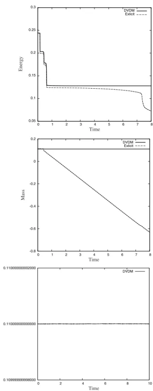
In this section we show that the proposed scheme (2.10) has the same characteristic prop- erties, mass conservation and energy dissipation, as the original problem (1.1)–(1.3) has.

Definition 4.1.

The total mass of U = ( U

,..., U

)

∈

is defined by M

( U ) : = ∑

k=0

U

x = U , 1 .

Theorem 4.2.

The scheme (2.10) has mass-conservation and energy-dissipation proper- ties in the sense that for all m = 0,1,...,

M

( U

) = M

( U

), (4.1) J

( U

) ≤ J

( U

). (4.2) Proof. By (2.10) and Lemma 2.3,

M

( U

) − M

( U

)

t = U

− U

t , 1

!

=

− A

J

δ

( U

, U

) , 1

=

−

J

δ

( U

, U

) , A1

= 0 . The last equality follows from the fact that

= ( 1 / √

L ) 1 is an eigenvector of A with eigenvalue 0. Thus we obtain (4.1).

Next we show (4.2). By (3.2) and (2.10), J

( U

) − J

( U

)

t =

J

δ

( U

, U

) , U

− U

t

!

=

δ

J

δ

( U

, U

) ,− A

J

( U

, U

)

≤ 0 .

The last inequality follows from the positive semi-definiteness of A. The theorem is proved.

5 Stability of the proposed scheme

In this paper, we use the following norms on

induced by the inner product ·,· . U

d

:=

"

N k

∑

| U

|

x

#_1/2

= U,U

, U

: = max

0≤k≤N

| U

|, U

d

: =

U , U + 1

2 ( D

U , D

U + D

U , D

U )

=

U , U +

A

U , A

U

.

The following lemma gives relations between above norms:

Lemma 5.1.

√ 1 L U

d

≤ U

≤ max

$

3 L ,

$

3L 2

%

U

d

.

Proof. Since Nx = L, U

d

≤ U

"

N k

∑

x

#1/2

= √

L U

.

This proves the first inequality.

Let K ∈ { 0 ,..., N } be such that | U

| = min

| U

| . Then, arguing as above, we obtain

| U

| ≤ 1

√ L U , U

. Since

U

− U

=

⎧⎪

⎪⎪

⎨

⎪⎪

⎪⎩

j−1 k

∑

( U

− U

), j > K ,

−

∑

k=j

( U

− U

), j < K , we have for j = 0 ,..., N,

|U

| ≤ |U

| +

∑

k=0

U

− U

x

x

≤ | U

| +

"

N−1 k

∑

U

− U

x

2

x

#1/2"

N−1 k

∑

x

#1/2

≤ 1

√ L U , U

+ √

L D

U , D

U

. We also have

| U

| ≤ 1

√ L U , U

+ √

L D

U , D

U

for j = 0 ,..., N in a similar manner. Combining these inequalities, we obtain U

≤ 1

√ L U , U

+

√ L 2

D

U , D

U

+ D

U , D

U

≤ C

U , U +

A

U , A

U

with C = max {

3 / L ,

3L / 2 } . Here the last inequality follows from the inequality

√ a + √ b + √

c ≤

3 ( a + b + c ) for a , b , c > 0. The lemma is proved.

The following result yields that the proposed scheme is numerically stable for any

time step:

Theorem 5.2.

The numerical solutions U

( m = 0 , 1 ,...) obtained by the proposed scheme (2.10) satisfy for all m ≥ 0,

U

d

≤

J

( U

) + 2L

, (5.1)

U

≤ C 2

ε²

J

( U

) + L

2 (ε

+ 2 )

(5.2) with C = max {

3 / L , 3L / 2 } . Proof. Since

W (u) = 1

4 (u

− 1)

≥ au

− a(a + 1) for a ∈

W ( U

), 1 ≥

a ( U

)

− a ( a + 1 ) 1 , 1 = a

U

, U

− a ( a + 1 ) L . (5.3) Therefore, Theorem 4.2 implies that for m ≥ 0,

J

( U

) ≥ J

( U

) ≥

W ( U

), 1 ≥

U

, U

− 2L . Here we take a = 1 in (5.3). Thus we obtain (5.1).

Similarly, taking a =

/ 2 in (5.3), we have for m ≥ 0, J

( U

) ≥ J

( U

) ≥

2

A

U

, A

U

+

W ( U

), 1

≥

2

A

U

, A

U

+

U

,U

−

4 (ε

+ 2) 1, 1

=

2 U

d

−

4 (ε

+ 2 ) L . Combining this with Lemma 5.1, we obtain

U

d

≤ C

2

ε²

J

( U

) + L

2 (ε

+ 2 )

with C = max { 3 / L ,

3L / 2 } . The theorem is proved.

6 Unique solvability of the scheme

In this section, we prove that the proposed scheme (2.10) has a unique solution U

. Let

:

×

→

be a map defined by

T

( U , V ) : = U − t 2 A

ε²

AV + g ( U , V ) − V

− t

2

V − V ), (6.1)

where g ( u , v ) : = u

v − 2uv

+ 2v

is a cubic function. Then, if

( U

,·) :

→

has a fixed point V

, then U

: = 2V

− U

is a solution of (2.10).