Output Feedback Strict Passivity of Discrete-time Nonlinear Systems and Adaptive Control System Design with a PFC,1
Ikuro Mizumotoa, Satoshi Ohdairaa, Zenta Iwaib
aDepartment of Intelligent Mechanical Systems, Kumamoto University, 2-39-1 Kurokami, Kumamoto, 860-8555, Japan
bKumamoto Prefectural College of Technology, 4455-1 Haramizu, Kikuyo-mach, Kikuchi-gun, Kumamoto, 869-1102, Japan
Abstract
In this paper, a passivity-based adaptive output feedback control for discrete-time nonlinear systems is considered. Output Feedback Strictly Passive (OFSP) conditions in order to design a stable adaptive output control system will be established.
Further a design scheme of a parallel feedforward compensator (PFC) which is introduced in order to realize an OFSP controlled system will be provided and an adaptive output feedback control system design scheme with a PFC will be proposed.
Key words: Adaptive control; discrete nonlinear systems; strict passivity; output feedback; parallel feedforward compensator.
1 Introduction
Since many practical systems contain some kind of non- linearities, a great deal of attention has been attracted to the control of nonlinear systems. Especially, of par- ticular interest are passivity based controller designs for the control problem on nonlinear systems (Hill and Moylan, 1998; Byrnes et al., 1991; Krstic et al., 1994;
Jiang and Hill, 1998; Fradkov and Hill, 1998; Byrnes and Lin, 1994; Lin and Byrnes, 1995). Although several important results have been obtained concerning pas- sivity based controls, most of the results however were ones for continuous-time systems (Hill and Moylan, 1998; Byrneset al., 1991; Krsticet al., 1994; Jiang and Hill, 1998; Fradkov and Hill, 1998). Our interest here is a discrete-time passive (or strictly passive) system. For discrete-time nonlinear systems, passivity properties has been investigated widely (Byrnes and Lin, 1994;
Lin and Byrnes, 1995; Monaco and Normand-Cyrot, 1997; Navarro-Lopezet al., 2002; Navarro-Lopez, 2007;
Monacoet al., 2008), however, only few passivity based The material in this paper was partially presented at 17th IFAC World Congress, Seoul, July 6-11, 2008. Corresponding author I. Mizumoto. Tel. +81-96-342-3759. Fax +81-96-342- 3729.
Email addresses: [email protected](Ikuro Mizumoto),[email protected](Zenta Iwai).
1 This work was partially supported by KAKENHI, the Grant-in-Aid for Scientific Research (C) 18560439, from the JapanSociety for the Promotion of Science (JSPS).
controls have been investigated with respect to loss- less or passive systems (Byrnes and Lin, 1994; Lin and Byrnes, 1995; Chellaboina and Haddad, 2002; Navarro- Lopez et al., 2002; Navarro-Lopez, 2007). In Byrnes and Lin (1994); Lin and Byrnes (1995); Chellaboina and Haddad (2002) feedback lossless or passivity were developed and stabilization of discrete-time nonlinear systems were investigated for input affine systems. In Navarro-Lopez et al. (2002); Navarro-Lopez (2007), dissipativity and/or passivity for general discrete-time nonlinear systems have been investigated and feedback passivity has also been developed. However, most these known results are related only to properties via state feedback. Considering the control design with a sim- ple structure in view of practical application, it seems useful and valuable to investigate the output feedback passivity properties and to establish passivity-based output feedback control for discrete nonlinear systems.
In this paper, we consider a passivity-based adaptive output feedback control for discrete-time nonlinear sys- tems. The passivity-based control schemes can be con- sidered one of the Lyapunov-based controls. As for the Lyapunov-based adaptive controls, several significant re- sults have been provided for discrete-time non-linear sys- tems(Hayakawa et al., 2004). However, the developed methods were also only with state feedback forms. Unlike the former works on the passivity-based control and the Lyapunov-based adaptive control, the passivity-based adaptive control dealt with in this paper is an output feedback-based adaptive control in which only the out-
put signal is utilized in the controller design. It is well known that one can easily design an output feedback based adaptive control for an output feedback strictly (exponentially) passive (OFSP) system (Jiang and Hill, 1998; Fradkov and Hill, 1998; Michinoet al., 2003; Mizu- motoet al., 2005) and the obtained control system has a strong robustness with respect to disturbances and un- certainties. Its simple structure of the adaptive controller and robustness are useful for practical applications. This is a motivation of this research.
The system is said to be OFSP if there exists an out- put feedback such that the resulting closed loop system is strictly passive. Here we investigate the OFSP prop- erty of discrete-time nonlinear systems, and consider an output feedback-based adaptive control design prob- lem for discrete-time nonlinear systems. To this end, we first derive a discrete-time nonlinear version of Kalman- Yakubovich-Popov (KYP) Lemma for a strictly pas- sive system. The strict passivity of the control system plays an important role in adaptive controls. The KYP- Lemma for continuous-time nonlinear systems has been interpreted (Hill and Moylan, 1998; Jiang and Hill, 1998) and the KYP-Lemma for discrete-time nonlinear sys- tems has been investigated for lossless and passive sys- tems (Byrnes and Lin, 1994; Lin and Byrnes, 1995).
Recently, KYP-Lemma for discrete-time nonlinear sys- tems is further investigated in relation to QS (Quadratic Storage)-passivity (Navarro-Lopez, 2007). Here, we will pay attention to the KYP-Lemma for strictly passive discrete-time nonlinear systems in order to design an adaptive control system. After that, OFSP conditions for discrete-time nonlinear systems will be clarified, and the design of output feedback-based adaptive control will be shown. As it is well known, a passive discrete-time system must have a direct feedthrough term of input, that is, a passive system must have a relative degree of 0 (Byrnes and Lin, 1994). This indicates that the OFSP system also has to have a direct feedthrough term of the input (i.e. relative degree of 0). Since most practi- cal systems do not have a direct feedthrough term of the input, the OFSP condition provides severe restrictions for practical applications of the considered adaptive de- sign scheme. The introduction of a parallel feedforward compensator (PFC) will be considered in order to alle- viate OFSP condition and it is shown that there exists a PFC which renders the augmented system with the PFC OFSP if the system can be stabilizable by a dynamic feedback. The inverse system of the dynamic controller can be a PFC. Further an adaptive output feedback con- trol system design with a PFC will be developed. The OFSP condition which the system must have a relative degree of 0 possibly results in a causality problem in the controller design. A condition in which one can design the adaptive controller without causality problems will be provided as strong output feedback strict passivity, and according to the obtained conditions, an adaptive output feedback controller design scheme will be shown for a discrete-time nonlinear system with a PFC.
2 Preparation: Strict passivity
Consider the following n-th order discrete-time SISO nonlinear system with a relative degree of 0.
x(k+ 1) = f(x(k)) +g(x(k))u(k)
y(k) = h(x(k)) +J(x(k))u(k) (1) wherex(k)∈Rnis a state vector,u(k),y(k)∈Rare the input and output of the system. f(x(k)) : Rn → Rn, g(x(k)) : Rn → Rn, h(x(k)) : Rn → R and J(x(k)) : Rn→Rare smooth inx(k), and we assume thatf(0) = 0,h(0) = 0.
The passivity and the strict passivity of the system (1) are defined as follows (Byrnes and Lin, 1994):
Definition 1 (Passivity) A system(1)is said to be pas- sive if there exists a non-negative function V(x(k)) : Rn→RwithV(0) = 0, called the storage function, such that
V(x(k+ 1))−V(x(k))≤y(k)u(k) (2) for allu(k)∈R,∀k≥0.
Definition 2 (Strict Passivity) A system(1)is said to be strictly passive if there exists a non-negative function V(x(k)) :Rn→RwithV(0) = 0and a positive definite functionS(x(k)) :Rn→Rsuch that
V(x(k+ 1))−V(x(k))≤y(k)u(k)−S(x(k)) (3) for allu(k)∈R,∀k≥0.
The property of a passive or lossless system has been studied in Byrnes and Lin (1994); Lin and Byrnes (1995).
Here we first investigate the strict passivity by means of the discrete-time nonlinear version of the KYP-Lemma in order to develop the adaptive controller for discrete- time nonlinear systems.
Theorem 1 A system(1)is strictly passive if and only if, there exists a non-negative functionV(x(k)) :Rn → RwithV(0) = 0such that
A1-1) There exist functions l(x),W(x) and a positive definite functionS(x)such that
V(f(x))−V(x) =−l(x)2−S(x) (4)
∂V(α)
∂α
α=f(x)
g(x) =h(x)−2l(x)W(x) (5) gT(x) ∂2V(α)
∂α2
α=f(x)
g(x) = 2J(x)−2W(x)2. (6) A1-2)V(f(x) +g(x)u)is quadratic inu.
Proof: The proof can be seen in Navarro-Lopez (2007) in relation to the QS-passivity. A specific proof for the strict passivity is given in Appendix A.
Remark 1: In Navarro-Lopez et al. (2002); Navarro- Lopez (2007), general discrete-time nonlinear systems have been dealt with in relation to KYP lemma. How- ever, in order to establish the basic concept of the fol- lowing passivity-based output feedback controls, here in this paper, the input affine system is dealt with.
3 Output feedback strict passivity
Next, we define an output feedback strict passivity for a system (1).
Definition 3 (Output feedback strictly passive: OFSP) A system(1)is said to be output feedback strictly passive (OFSP) if there exists an output feedback:
u(k) =α(y(k)) +β(y(k))v(k) (7) such that the resulting closed loop system is strictly pas- sive.
Further we define a strong output feedback strict pas- sivity as follows:
Definition 4 (Strongly OFSP) A system(1)is said to be strongly OFSP if the system is OFSP with a static output feedback, i.e. there exists a static output feedback:
u(k) =−θ∗y(k) +v(k), θ∗ >0 (8) such that the resulting closed loop system fromy(k)to v(k),
x(k+ 1) = ¯f(x(k)) + ¯g(x(k))v(k)
y(k) = ¯h(x(k)) + ¯J(x(k))v(k) (9) with
f¯(x(k))=f(x(k))− θ∗
1+θ∗J(x(k))h(x(k))g(x(k)) (10)
¯
g(x(k))= 1
1+θ∗J(x(k))g(x(k)) (11)
¯h(x(k))= 1
1+θ∗J(x(k))h(x(k)) (12) J(x(k))=¯ 1
1+θ∗J(x(k))J(x(k)) (13) is strictly passive and, in addition, a transformed closed loop system with
¯
v(k) = 1
1 +θ∗J(x(k))v(k) (14)
as input,
x(k+ 1) = ¯f(x(k)) +g(x(k))¯v(k)
y(k) = ¯h(x(k)) +J(x(k))¯v(k) (15) is also strictly passive.
Remark 2:In Definition 4, it should be 1 +θ∗J(x)= 0,
∀x∈R, so that the system to be strongly OFSP globally.
For linear discrete-time systems, this strongly OFSP is recognized as strongly almost strictly positive real (strongly ASPR) (Mizumotoaet al., 2007).
The sufficient conditions for a system (1) to be OFSP are provided by the following theorem.
Theorem 2 A system (1) is OFSP with a static output feedback (8) and aC2positive definite storage function if
A2-1) The system has relative degree of 0 andJ(x(k))>
0,∀x(k).
A2-2) The zero dynamics of the system:
x(k+ 1) =f∗(x(k)) (16)
is asymptotically stable with the followingC2pos- itive definite functionV satisfying
a)V(f∗(x))−V(x) =−ζ(x) (17) with a positive definite functionζ(x).
b)V(f∗(x) +g(x)u) is quadratic in u.
c) There exist positive definite matrices Γm,ΓM
such that
0<Γm≤ ∂2V(α)
∂α2
α= ¯f(x(k))≤ΓM (18) A2-3) gJ((xx((kk)))) is bounded.
Proof: The zero dynamics of the system(1) is obtained by (Byrnes and Lin, 1994)
x(k+ 1) =f∗(x(k)) =f(x(k))−h(x(k))
J(x(k))g(x(k)) (19) Since ¯f(x) in the closed loop system (9) can be repre- sented from (10) and (19) by
f¯(x) =f(x)− θ∗
1 +θ∗J(x)h(x)g(x)
=f∗(x) + ˜J(x)h(x)g(x) (20) with
J˜(x) = 1
J(x) (1 +θ∗J(x)), (21)
from assumption A2-2), b),V( ¯f(x)) can be expressed as V( ¯f(x)) =V(f∗(x)) + ˜J(x)h(x) ∂V(α)
∂α
α=f∗(x)
g(x) +1
2J(x)˜ 2h(x)2gT(x) ∂2V(α)
∂α2
α=f∗(x)
g(x).
(22) Thus we have from (17),(22) that
V( ¯f(x))−V(x)
=−ζ(x) + ˜J(x)h(x) ∂V(α)
∂α
α= ¯f(x)
g(x)
−1
2J˜(x)2h(x)2gT(x) ∂2V(α)
∂α2
α= ¯f(x)
g(x). (23) Now, consider a function ¯W(x) that satisfies the follow- ing relation:
W¯(x)2= ¯J(x)−1
2¯gT(x) ∂2V(α)
∂α2
α= ¯f(x)
¯
g(x). (24) Such function ¯W(x) is certain to exist for a sufficiently largeθ∗from assumptions A2-2),c) and A2-3). Further, consider a function ¯l(x(k)) that satisfies
∂V(α)
∂α
α= ¯f(x)
¯
g(x) = ¯h(x)−2¯l(x) ¯W(x). (25) Since (25) yields that
¯l(x)2W¯(x)2=1 4
¯h(x)2−2¯h(x) ∂V(α)
∂α
α= ¯f(x)
¯ g(x)
+
∂V(α)
∂α
α= ¯f(x)
¯ g(x)
2
, (26) we have from (24) and (26) that
¯l(x)2
J(x)¯ −1
2¯gT(x) ∂2V(α)
∂α2
α= ¯f(x)
¯ g(x)
=1 4
¯h(x)2−2¯h(x) ∂V(α)
∂α
α= ¯f(x)
¯ g(x)
+
∂V(α)
∂α
α= ¯f(x)
¯ g(x)
2
. (27)
Thus, we obtain from (27) that
¯h(x) ∂V(α)
∂α
α= ¯f(x)
¯ g(x)
=−2¯l(x)2
J¯(x)−1
2¯gT(x)∂2V(α)
∂α2
α=¯f(x)
¯ g(x)
+1 2
¯h(x)2+
∂V(α)
∂α
α= ¯f(x)
¯ g(x)
2
. (28) Furthermore, taking the definitions of ¯g(x) and ¯h(x) in (11) and (12) in to account, we have from (28) that h(x) ∂V(α)
∂α
α= ¯f(x)
g(x)
=−2¯l(x)2
(1+θ∗J(x))J(x)−1
2gT(x)∂2V(α)
∂α2
α= ¯f(x)
g(x)
+1 2
h(x)2+
∂V(α)
∂α
α= ¯f(x)
g(x) 2
. (29) Therefore, we obtain from (23) and (29) that
V( ¯f(x))−V(x)
=−ζ(x)−2¯l(x)2
+ 1
J(x) (1 +θ∗J(x)) 1
2 h(x)2
+
∂V(α)
∂α
α= ¯f(x)
g(x) 2
+
¯l(x)2−1 2
1
J(x) (1 +θ∗J(x))h(x)2
×gT(x) ∂2V(α)
∂α2
α= ¯f(x)
g(x)
. (30)
Finally, we have
V( ¯f(x))−V(x) =−¯l(x)2−S(x)¯ (31) where
S(x) =¯ ζ(x) + ¯l(x)2
− 1
J(x) (1 +θ∗J(x)) 1
2 h(x)2
+
∂V(α)
∂α
α= ¯f(x)
g(x) 2
+
¯l(x)2−1 2
1
J(x) (1 +θ∗J(x))h(x)2
×gT(x) ∂2V(α)
∂α2
α= ¯f(x)
g(x)
. (32)
S(x(k)) is certain to be a positive definite function with¯ a sufficiently largeθ∗. Thus we can conclude that, for a
sufficiently largeθ∗, there exists a positive definite C2 functionV(x) with a property thatV(f(x) +g(x)u) is quadratic inu, functions ¯W(x(k)), ¯l(x) and a positive definite function ¯S(x(k)) such that
V( ¯f(x))−V(x) =−¯l(x)2−S(x)¯ (33)
∂V(α)
∂α
α= ¯f(x)
¯
g(x) = ¯h(x)−2¯l(x) ¯W(x) (34)
¯
gT(x) ∂2V(α)
∂α2
α= ¯f(x)
¯
g(x) = 2 ¯J(x)−2 ¯W(x)2, (35) that is there exists a feedback gainθ∗ such that the re- sulting closed loop system is strictly passive. Then the system is output feedback strictly passive with aC2pos- itive definite function as the storage function.
Remark 3:The conditions A2-1) and A2-2) (b) are nec- essary conditions to be OFSP. These conditions can be seen in Byrnes and Lin (1994) as necessary conditions on the feedback equivalent to lossless system. The con- ditions A2-2)(a), (c) and A2-3) are conditions for the existence of a static output feedback which renders the resulting system strictly passive. Note that the condi- tion 0≤ ∂2V(α)
∂α2
α= ¯f(x(k))
is one of the conditions with which there exists a smooth state feedback such that the resulting closed system is globally asymptotic stable (Byrnes and Lin, 1994).
Moreover, we have the following lemma concerning the strongly OFSP conditions.
Lemma 1 Assumptions A2-1), A2-2) and A2-3) in Theorem2are satisfied withJ(x(k)) = d > 0then the system(1)is strongly OFSP.
Proof: See appendix B.
The derived OFSP and/or strong OFSP conditions are very restrictive for practical systems, since most practi- cal systems do not have relative degree of 0 and it is diffi- cult to choose adequate sampling period with which the system is minimum-phase. In the following section, we first show that there exists a parallel feedforward com- pensator (PFC) which renders the augmented system with the PFC OFSP, and then the passivity-based adap- tive output feedback design for the OFSP augmented system with a PFC will be proposed.
4 Realization of OFSP system
Consider the following system withJ(x) = 0 in (1):
x(k+ 1) = f(x(k)) +g(x(k))u(k)
y(k) = h(x(k)). (36)
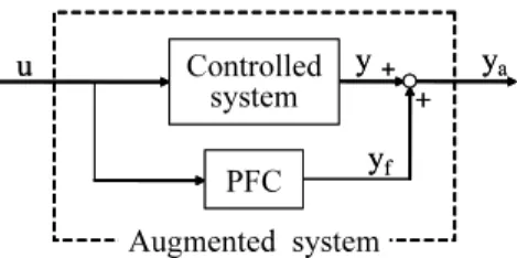
+ + Controlled
system PFC Augmented system
y ya
yf
u +
+ Controlled
system PFC Augmented system
y ya
yf u
Fig. 1. Block diagram of the augmented system with a PFC This system is not OFSP, so we consider introduction of a PFC:
xf(k+ 1) =Afxf(k) +bfu(k)
yf(k) = cTfxf(k) +du(k). (37) which is implemented in parallel with the controlled sys- tem (36) as shown in Fig. 1, so as to make the resulting augmented system OFSP.
The resulting augmented system can be expressed by xa(k+ 1) = fa(xa(k)) +ga(xa(k))u(k)
ya(k) = y(k) +yf(k) =ha(xa(k)) +du(k). (38) where
xa(k) = x(k)
xf(k)
, fa(xa(k)) =
f(x(k)) Afxf(k)
ha(xa(k)) =y(k) +cTfxf(k) =h(x(k)) +cTfxf(k)
The PFC (37) has to be designed such that the resulting augmented system (38) is OFSP. Concerning the exis- tence of such a PFC and design scheme of the PFC, we have the following theorem.
Theorem 3 Assume that the system (36) can be stabi- lized with aC2positive definite functionV by a dynamic feedback given by
xd(k+ 1) =Adxd(k) +bdy(k) yd(k) =cTdxd(k) +ddy(k) u(k) =−yd(k)
(39)
Consider the inverse system of (39) with u(k) as input andyf(t) =−y(k) as output expressed by
xf(k+ 1) = (Ad−d1dbdcTd)xf(k)−d1dbdu(k) yf(k) = d1
dcTdxf(k) +d1
du(k) (40)
and consider an augmented system with this as a PFC as shown in Fig. 1. Then the zero dynamics of the aug-
mented system is stable with the C2 positive definite functionV.
Proof: The closed loop system with u(k) = −yd(k) as the control input can be represented by
x(k+ 1) xd(k+ 1)
=
f(x(k)) Adxd(k)
+
−g(x(k))(cTdxd(k) +ddy(k)) bdy(k)
=
f(x(k))−g(x(k))cTdxd(k) Adxd(k)
+
−ddg(x(k))y(k) bdy(k)
(41) This is a stable system from assumption.
Now, let’s consider the inverse system of (39) withu(t) as the input andyf(k) =−y(k) as the output. The inverse system can be given in (40). The augmented system with the inverse system (40) as a PFC is then expressed by x(k+ 1)
xf(k+ 1)
=
f(x(k))
(Ad−d1
dbdcTd)xf(k)
+
g(x(k))
−d1
dbd
u(k)
(42) ya(k) =h(x(k)) +yf(k)
=y(k) + 1 dd
cTdxf(k) + 1 dd
u(k) (43)
The zero dynamics of this augmented system is then obtained by
x(k+ 1) xf(k+ 1)
=
f(x(k))
(Ad−d1
dbdcTd)xf(k)
+
g(x(k))
−d1
dbd
(−cTdxf(k)−ddy(k))
=
f(x(k))−g(x(k))cTdxf(k) Adxf(k)
+
−ddg(x(k))y(k) bdy(k)
(44) This zero dynamics have the same structure as in (41).
Thus the zero dynamics of the resulting augmented sys- tem is stable withC2 positive definite functionV. This theorem indicates that if a controller which stabi- lizes the system with aC2positive definite function V
satisfying the conditions given in Theorem 2, then de- signing the PFC as a inverse system of the system sta- bilizing controller, one can obtain a OFSP augmented system.
5 Adaptive output feedback controller design Assumption 4 (1) g(x(k)) is bounded for allx(k).
(2) There exists a known PFC given in (37) such that the resulting augmented system is rendered OFSP with a static output feedback, that is the aug- mented system (38) satisfies the OFSP conditions in the Theorem 2.
The objective here is to design an adaptive output feed- back control system under Assumption 4.
Under Assumption 4, (2), from Theorem 2 and Lemma 1, there exists a static output feedback:
u∗(k) =−θ∗ya(k) +v(k) (45)
for the augmented system (38), such that the resulting closed loop system with the transformed signal ¯v(k) = (1 +θ∗d)−1v(k) as the input:
xa(k+ 1) = ¯fa(xa(k)) +ga(xa(k))¯v(k)
ya(k) = ¯ha(xa(k)) +d¯v(k) (46)
f¯a(xa(k)) =fa(xa(k))− θ∗
1 +θ∗dha(xa(k))ga(x(k)) (47)
¯ha(xa(k)) = 1
1 +θ∗dy(k),¯ y(k) =¯ ha(xa(k)) (48) is strictly passive with a C2 positive definite storage function.
Thus, if one can design a control input by
u∗(k) =−θ∗ya(k), (49)
then a stable control system is obtained. However for a system with uncertainties, of course, θ∗ is unknown, and because of the existence a direct feedthrough term of the input, the input (49) can not be implemented due to causality problems.
To overcome these problems, we first consider the fol- lowing equivalent input obtained from (38):
u∗(k) =− θ∗
1+θ∗dy(k) =¯ −θ˜∗y(k),¯ θ˜∗= θ∗
1+θ∗d. (50) Then for this ideal control input, we design the control input adaptively as follows:
u(k) =−θ(k)¯˜ y(k) (51)
where the feedback gain ˜θ(k) is adaptively adjusted by the following parameter adjusting law:
θ(k) = ˜˜ θ(k−1) +γya(k)¯y(k), γ >0. (52) In this case, the augmented outputya(k) can be obtained from (38) by
ya(k) =
1−dθ(k˜ −1)
¯ y(k)
1 +dγy(k)¯ 2 (53)
without causality problems. It should be noted that if the controller is designed based on the input (49), then causality problems will appear.
5.1 Stability analysis
The obtained closed loop system with the input (51) is expressed by
xa(k+ 1) = ˜fa(xa(k)) +ga(xa(k))∆u(k)
ya(k) = ˜y(k) +d∆u(k), (54)
where
f˜a(xa(k)) =fa(xa(k))−θ˜∗y(k)g¯ a(xa(k)) (55)
˜ y(k) =
1−dθ˜∗
¯
y(k) (56)
∆u(k) =−∆˜θ(k)y(k),∆˜θ(k) = ˜θ(k)−θ˜∗. (57) From the definition of ˜θ∗, we have
f˜a(xa(k)) =fa(xa(k))− θ∗
1 +θ∗dy(k)g¯ a(xa(k))
= ¯fa(xa(k)) (58)
˜ y(k) =
1− θ∗d 1 +θ∗d
¯
y(k) = 1
1 +θ∗dy(k)¯
= ¯ha(xa(k)). (59)
This means that the system (54) is strictly passive with C2positive definite storage function.
Thus, there exists a C2 positive definite function V1, functions l1(xa(k)),W1(xa(k)), and a positive definite functionS1(xa(k)) such that
C1) V1( ¯fa(xa))−V1(xa) =−l1(xa)2−S1(xa)
∂V1(α)
∂α
α= ¯fa(xa)
g(x) = ¯ha(xa)−2l1(xa)W1(xa) gaT(xa) ∂2V1(α)
∂α2
α= ¯fa(xa)
ga(xa) = 2d−2W1(xa)2 C2) V1( ¯fa(xa) +ga(xa)∆u) is quadratic in ∆u.
Therefore, considering the difference ofV1(xa(k)), it is easy to show that we have
V1(xa(k+ 1))−V1(xa(k))
=ya(k)∆u(k)−S1(xa(k))
−(l1(xa(k)) +W1(xa(k))∆u(k))2. (60)
Now, consider the following positive definite functionV: V(k) =V1(xa(k)) +V2(k) (61) V2(k) = 1
2γ∆˜θ(k−1)2. (62)
Define a difference ∆V(k) as
∆V(k) =V(k+ 1)−V(k)
= ∆V1(xa(k)) + ∆V2(k) (63)
∆V1(xa(k)) =V1(xa(k+ 1))−V1(xa(k)) (64)
∆V2(k) =V2(k+ 1)−V2(k). (65)
The difference ∆V2(k) is represented by
∆V2(k) = 1 2γ
∆˜θ(k)2−∆˜θ(k−1)2
. (66)
Since we have from (52) that
∆˜θ(k−1) = ∆˜θ(k)−γya(k)¯y(k), (67) we obtain
∆V2(k) =−∆u(k)ya(k)−1
2γya(k)2y(k)¯ 2. (68) Consequently, the difference ∆V can be evaluated from (60) and (68) by
∆V(k) =−S1(xa(k))−(l1(xa(k)) +W1(xa(k))∆u(k))2
−1
2γya(k)2y(k)¯ 2
≤ −S1(x(k))≤0. (69)
From this result, we can conclude that all the signals in the control system are uniformly bounded. Further, from (69), we have limk→∞xa(k) = 0. Thus we obtain limk→∞y(k) = 0.
Finally, we have the following theorem.
Theorem 5 Under the Assumption 4, all the signals in the resulting closed loop control system with control input in (51) are uniformly bounded, and lim
k→∞y(k) = 0 is achieved.