Observational study on nocturnal cooling in a complex of small valleys in the western margin of Kanto Plain during the winter

(1)

Observational study on nocturnal cooling in a complex of small valleys in the western

margin of Kanto Plain during the winter

Shohei KONNO

Department of Geography,

Graduate School of Urban Environmental Science, Tokyo Metropolitan University

September 2013

(2)

i

List of Figures

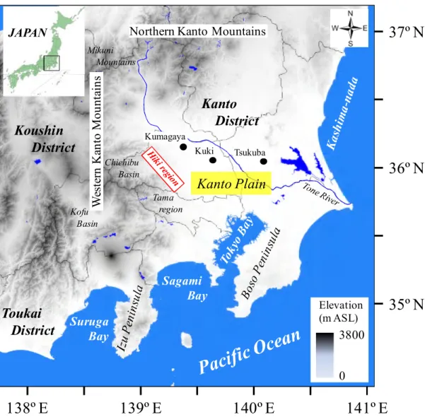
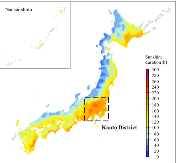
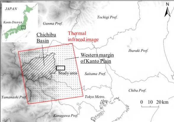
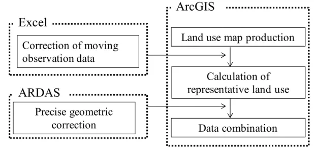
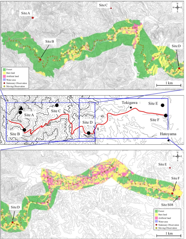
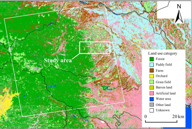
Fig. 1 Location and topography of the Kanto Plain. ... 53 Fig. 2 Monthly climate normal of total sunshine duration (hours) in January, calculated by the Japan Meteorological Agency (JMA) by using the observed data from 1981 to 2010. ... 54 Fig. 3 Upper and Middle: Location and topography of the study area, and the distribution of the sites used for horizontal measurements (circles), measurements at multiple heights (diamonds), and kytoon measurements (star). Red line is the route of moving observation. Lower: Cross-section of the topography along the X-Y line shown in the middle figure. ... 55 Fig. 4 Map of coverage of the Terra/ASTER thermal image (Red square), the western margin of the Kanto Plain (dot area), and the Chichibu Basin (shaded area). ... 62 Fig. 5 Data processing procedure for calculating the validity of the surface temperature of the satellite image. ... 63 Fig. 6 Land-use maps along the moving observation route shown in the upper panel of Fig. 3, reflecting the actual land covers. ... 64 Fig. 7 Land-use map by the Natural Environment Information GIS. White square indicates coverage of the Terra/ASTER thermal image. ... 66 Fig. 8 Relationship of minimum nighttime temperatures on clear nights between (a) the Hatoyama and Kuki AMeDAS stations, and (b) the Hatoyama AMeDAS station and the Kumagaya Local Meteorological Observatory from 1 January 2008 to 31 December 2012. ... 67 Fig. 9 Relationship of daily maximum temperatures on clear nights between (a)

(5)

iv

the Hatoyama and Kuki AMeDAS stations, and (b) the Hatoyama AMeDAS station and the Kumagaya Local Meteorological Observatory from 1 January 2008 to 31 December 2012. ... 68 Fig. 10 Relationship of nighttime minimum temperatures measured at the Hatoyama and Kuki AMeDAS stations on clear nights when the mean wind speed at both stations was less than 1 m s⁻¹ during the winter seasons from 1 January 2008 to 31 December 2012. ... 69 Fig. 11 Intraseasonal changes in the maximum inversion index from 1 December 2010 to 28 February 2011. The symbol below each date describes the weather conditions on that date as reported by the Kumagaya Local Meteorological Observatory of the JMA. ... 70 Fig. 12 Relationship of wind speeds between the Hatoyama AMeDAS station and site G when the temperature lapse rate was positive (i.e., when TG – TAMeDAS

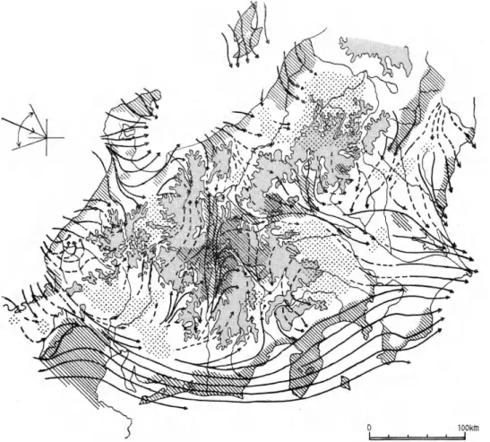
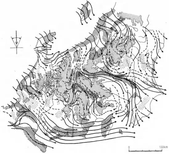
< 0) and the prevailing wind directions at site G were (a) northerly and (b) northwesterly on nights from 26 December 2010 to 19 March 2011. ... 71 Fig. 13 Prevailing wind direction at site G on nights from 26 December 2010 to 19 March 2011 when the temperature lapse rate was positive (i.e., when TG – TAMeDAS < 0). ... 72 Fig. 14 Distribution of surface wind on the central Japan in winter season (Type I). Illustration: streamline; solid line (apparent prevailing wind direction) broken line (weak wind): shaded area; mountainous region: dotted area; calm area: hatched area; area with prevailing strong wind (Kawamura, 1966). .... 74 Fig. 15 Same as Fig. 14 (Type II). ... 75 Fig. 16 Same as Fig. 14 (Type III). ... 76 Fig. 17 Same as Fig. 14 (Type IV). ... 77

(6)

v

Fig. 18 A weather map for the pressure pattern classification (after Japan Surface Weather Charts of JMA). ... 78 Fig. 19 Wind distribution map for the pressure pattern classifications. “C”

represents calm conditions (wind speed is less than 0.3 m s^-1), and a red square and black circle above the “C” indicate the meteorological observatory and the AMeDAS site, respectively. ... 79 Fig. 20 Pressure pattern transition during the winter (from 1 December 2010 to 28 February 2011). ... 81 Fig. 21 Mean wind distributions for Types I, II, III, and H from 1 December 2010 to 28 February 2011. ... 82 Fig. 22 Relationship of wind speed between sites G and H at (a) nighttime and (b) daytime from 10 February 2011 to 19 March 2011. Data shown in figure is 1 hour mean value. ... 83 Fig. 23 Weather map on the night of 22 February, 2011 12:00 UTC (Surface Weather Charts of JMA). ... 85 Fig. 24 Temporal variation in air temperature and wind speed on the night of 22 February, 2011. The symbol described above represents the weather conditions at 15:00, 21:00 JST, and 09:00 JST on the following day, as reported by the Kumagaya Local Meteorological Observatory of the JMA (Open circles indicate clear weather conditions). ... 86 Fig. 25 Thermal infrared image observed by thermography at the location of the thermography site on 23 February 2011, 01:45 JST. The upper left part of the figure shows the visible image at the same location. ... 87 Fig. 26 Vertical distributions of (a) surface temperature measured by thermography on 23 February, 2011 01:45 JST, (b) air temperature measured

(7)

vi

by the data-logger on 23 February, 2011 01:40 JST. ... 88 Fig. 27 Weather map on the night of 27 December, 2010 12:00 UTC (Surface Weather Charts of JMA). ... 89 Fig. 28 Temporal variations in (a) wind speed and (b) air temperature from 27 December, 2010 15:00 JST to 28 December, 2010 09:00 JST. Missing data in wind speed at Site A until 16:30 JST. ... 90 Fig. 29 Cross-section of (a) satellite-estimated surface temperature and ground-observed air temperature along the moving observation route on the night of 27 December 2011, (b) elevation and representative land use (green:

forest, yellow: bare land, red: artificial land) along the moving observation route (red line in Fig. 3). F-d: Dominant forest area. B-d: Dominant bare area.

A-d: Dominant artificial area. Vertical gray bands represent the absence of dominant areas. ... 91 Fig. 30 Frequency distribution of the difference of satellite-estimated surface temperature and ground-observed air temperature. ... 92 Fig. 31 Temporal variation in air temperature (Ta), surface temperature (Ts), and their differences (⊿T = Ts －Ta) at site F (from 27 December, 2010 12:00 JST to 28 December, 2010 12:00 JST). The vertical red line indicates the time when a satellite passed above the study area (21:54 JST). ... 94 Fig. 32 Upper: Terra/ASTER thermal infrared image acquired on 27 December, 2010, 21:54 JST. Lower: Topography and coverage of the image. ... 95 Fig. 33 Vertical distribution of (a) satellite-observed surface temperature in the western margin of the Kanto Plain (dot area in Fig. 4) on 27 December, 2010, 21:54 JST, and (b) air temperature measured by the data-logger on 27 December, 2010, 21:50 JST. ... 96

(8)

vii

Fig. 34 Time series of differences between temperature at each mountain points (sites A, B, C, E, and S22) and that at site S17 on clear and calm nights (mean values for 9 days on 27 December 2010; 8, 14, 17, and 31 January, 3 and 21 February, and 5 and 13 March 2011). ... 97 Fig. 35 Diurnal variability in radiation fluxes at site F under clear and calm days (mean value for 4 days on 14 January, 21 February, and 5 and 13 March 2011). ... 98 Fig. 36 Horizontal distribution of mean (a) evening temperature (Teve), (b) daily minimum temperature (Tmin), and (c) nocturnal cooling (Tnoc = Teve – Tmin) under clear and calm conditions. ... 99 Fig. 37 Temporal variation in wind speed and direction measured at the Hatoyama AMeDAS station on the nights of 29 February and 7 March 2008.

101

Fig. 38 (a, b) Vertical profiles of air temperature measured by the kytoon system at site S17 and (c, d) vertical cross-sections showing the isothermal distribution of potential temperature along valley V1 on the night of 29 February and early morning of 1 March 2008. ... 102 Fig. 39 (a, b) Vertical profiles of air temperature measured by the kytoon system at site S17 and (c, d) vertical cross-sections showing the isothermal distribution of potential temperature along valley V1 on the night of 7 March and early morning of 8 March 2008. ... 103 Fig. 40 Vertical distribution of temperature decrease after sunset on the slope of western Kanto Mountain on clear and calm nights (mean value for 7 days on 17 and 27 December 2010 and 8 and 14 January, 21 February, and 5 and 13 March 2011). ... 104

(9)

viii

Fig. 41 Time variation in mean (a) frequency and wind speed of the cold air current, and (b) magnitude of inversion index on clear and calm nights (mean value for 7 days on 17 and 27 December 2010 and 8 and 14 January, 21 February, and 5 and 13 March 2011). ... 105 Fig. 42 Heat budget at ground level and in the air layer above the study area on clear and calm nights (mean value for 5 days on 8 and 14 January, 21 February, and 5 and 13 March 2011). ... 106 Fig. 43 Schematic diagrams illustrating cold air and radiation activities at early (left) and mid-night (right) phases in a basin or valley in (a) semi-mountainous area and (b) mountainous area. ... 107

(10)

ix

List of Tables

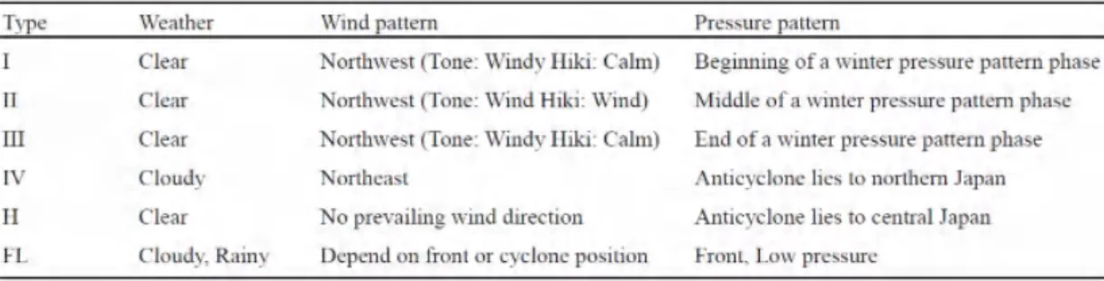
Table 1 Summary of meteorological measurements at sites A to H (from December 2010 to March 2011). ... 58 Table 2 Land-use categories. ... 65 Table 3 Features of weather, wind pattern, and pressure pattern in each type (after Kawamura, 1966) ... 73 Table 4 Anomalies of monthly mean temperature, precipitation, sunshine duration, and snowfall relative to 30-year average (1981–2010) during the winter season (from December 2010 to February 2011). ... 80 Table 5 Mean magnitude of temperature inversion index in each pressure pattern.

84

Table 6 Percentile value of the difference in satellite-estimated surface temperature and ground-observed air temperature for differing land uses. P25, P50, and P75 represent percentile values of 25%, 50%, and 75%, respectively.

93

Table 7 List of clear and calm nights during the winter season (from December 2007 to March 2008). ... 100

(11)

x

List of Pictures

Picture 1 Photograph of the horizontal temperature measurement site (A thermometer at site S09 with naturally ventilated radiation shield). ... 56 Picture 2 Photograph of the multiple height measurement site (thermometers at site T04 with naturally ventilated radiation shield). ... 57 Picture 3 Photograph of the wind measurement instruments (anemometer and thermometer) at site G. ... 59 Picture 4 Photograph of the comprehensive measurements of meteorological elements at site F. ... 60 Picture 5 Photograph of a kytoon measurement at the playground of the Hatoyama Junior High School. ... 61

(12)

1

Acknowledgment

I would like to express my gratitude to my supervisor, Professor Hideo Takahashi of Department of Geography, Tokyo Metropolitan University (Dept. Geog., TMU) for giving me insightful comments and suggestions that make my research of great achievement.

I am deeply grateful to Professor Jun Matsumoto (Dept. Geog., TMU) and Tomoko Nakano of Faculty of Economics, Chuo University for their constructive comments and considerable encouragement.

I also owe my deepest gratitude to Doctor Hiroharu Tanaka of Nagano Envi- ronmental Conservation Research Institute for his assistance during the observation.

Without his guidance and persistent help the observation would not have been possible.

The observation was supported by the Hatoyama and Tokigawa Town Office, Higashimatsuyama City Office, Higashimatsuyama Land Development Office, and Hatoyama Junior High School.

Finally, I greatly appreciate all members of the Laboratory of Climatology and Department of Geography, Tokyo Metropolitan University, as well as deeply grateful to my parents, family, and friends for their understanding, support, and warm encouragement.

(13)

2

Abstract

Numerous studies have suggested that cooling intensity is stronger in a basin or valley than in a flat, open area, because the mountain ridges surrounding a basin or valley block the ambient wind and enhance nocturnal cooling by decreasing the turbu- lent exchange. In addition, air cooled radiatively at ground level on the surrounding mountain slopes flows into the basin or valley and produces a strong inversion layer at a lower elevation.

However, previous studies of valleys in semi-mountainous areas have reported that in situ cooling and a wind-sheltering effect predominantly govern nocturnal cooling, and cold air flows play a less significant role. As a result, nocturnal cooling strength should be the same in a valley and on a nearby plain when the weather is clear and calm in both areas. The mechanism of nocturnal cooling in a basin or valley is well understood; however, little research has been reported regarding the equivalence of nocturnal cooling strength between a valley and its neighboring flat terrain. While numerous studies on nocturnal cooling have been carried out in basins or valleys in mountainous regions, research in semi-mountainous regions is limited to a few studies.

We clarify the nocturnal cooling mechanism in a complex of small valleys in a semi-mountainous region near the western margin of the Kanto Plain, Japan. We measured temperature, wind, humidity, air pressure, and radiation continuously throughout each winter from 2007 to 2011, and on clear, calm days, we carried out intensive observations and thermal infrared image analyses.

First, systematic changes in the strength of the seasonal wind associated with the life cycle of the winter pressure pattern (distribution of atmospheric pressure in which high pressure lies to the west and low pressure to the east) controlled nocturnal cooling

(14)

3

in the study area. At the beginning and end of the winter pressure pattern phase, strong winds were restricted to the northern or eastern areas of Saitama Prefecture, and winds were weak near the base of the western Kanto Mountains, causing nighttime low temperatures to be more frequent in the valleys than on flat parts of the plain. In these situations, however, the wind-sheltering effect of the surrounding ridges played only a minor role in nocturnal cooling. When clear and calm conditions prevailed over the entire Kanto Plain, minimum temperatures in the valley bottom were at least 1 to 2 °C lower than those on the plain. Under these conditions, cold air flowing downslope contributed to nocturnal cooling in the valley in the early evening. Subsequently, this cold air current was weakened by the increasing stability associated with the formation of an inversion layer. As the inversion developed, atmospheric radiation was reduced, which promoted radiative cooling in the valley bottom. This radiative cooling was the dominant factor accounting for nocturnal cooling for the rest of the night. The contri- butions of atmospheric radiative cooling and advective cooling to the observed cooling of the air layer were approximately 60% and 30%, respectively. The contribution of atmospheric radiation reduction induced by the formation of a temperature inversion layer to atmospheric radiative cooling was about 30%.

Previous studies of nocturnal cooling in small valleys in semi-mountainous areas have reported in situ cooling and a wind-sheltering effect to be the predominant factors governing nocturnal cooling, with cold air flows playing a less significant role.

These studies, therefore, inferred that the nocturnal cooling strength would be equivalent in a valley and in a neighboring flat area when weather conditions were clear and calm in both areas. In this study, however, we found that cold air flow, as well as in situ cooling, contributed to nocturnal cooling in a valley. As a result, we observed temperatures in the valley that were lower than those in a neighboring flat area.

(15)

4

1. Introduction

1.1 Background and objectives

Under calm wind conditions on a clear night in an area of flat terrain, air temperature near the ground surface drops remarkably due to radiative loss of heat on the ground surface (Whiteman et al., 2004). This radiative cooling of the air near the ground can cause a temperature inversion layer to form above the ground (Endo, 1961), which in turn decreases the downward longwave radiation toward the ground and promotes additional radiative cooling (Kondo and Yamazawa, 1983; Maki and Harimaya, 1988). The intensity of atmospheric cooling depends on topography as well as on weather and ground surface conditions. In a basin or valley, the surrounding mountains block the ambient wind and enhance nocturnal cooling by decreasing tur- bulent air exchange (Saito et al., 1966; Thompson, 1986). In addition, air that is cooled radiatively at ground level on the surrounding mountains flows downslope into the basin or valley, and its accumulation at lower elevations produces a strong inversion layer (Yoshino et al., 1981; Mori et al., 1983). For this reason, the cooling intensity in a basin or valley is stronger than that in an open, flat area (Kondo, 1984). Under very clear and calm conditions, the temperature in an enclosed area can fall as much as a few tens of Kelvin (e.g., Clements et al., 2003; Zängl, 2005).

However, previous studies of nocturnal cooling in valleys located in semi-mountainous areas have reported that in situ cooling and the wind-sheltering effect are the predominant factors governing nocturnal cooling, and that the downslope cold air flow played a less significant role (Tanaka et al., 1983; Matsuoka et al., 1987).

These studies concluded that the nocturnal cooling strengths should be equivalent between a valley and a neighboring flat area under clear and calm weather conditions in

(16)

5

both areas. While the mechanism of nocturnal cooling in a basin or valley is well understood, there has been little research regarding the equivalence of nocturnal cooling strength between a valley and nearby flat terrain.

In general, the speed of cold air flow into and down a valley is governed by the stability of temperature inversion as well as by the slope angle and length, and the ground roughness (Kondo, 2000). Kondo and Sato (1988) mathematically demon- strated that the speed of cold air flow decreases as atmospheric stability increases.

Some studies of nocturnal cooling in a basin have pointed out that the cold air flows directly toward the basin floor for a few hours after sunset, but subsequently the flow becomes weaker as atmospheric stability near the basin floor increases, and a portion of the drainage winds then flows over the top of the inversion layer (Magono et al., 1982; Maki et al., 1984; Fast et al., 1996). The thickness of the surface inversion layer above a flat terrain (e.g., on a plain) commonly reaches 150 to 250 m in Japan (Tohsha, 1953; Ota, 1960). According to Tanaka et al. (1983) and Matsuoka et al. (1987), val- leys in their study areas were about 50 m deep. Assuming that a ground-level inversion layer formed over the adjoining plain area, it could cover the entire valley. This strong stable inversion layer would then suppress downslope currents of cold air by the strong stable layer of the inversion. However, even in a small valley in a semi-mountainous area, cold air should play a role in nocturnal cooling for a few hours after sunset, before the valley becomes covered by a stable inversion layer. As a result, nocturnal cooling in the valley is likely to be stronger than that on a neighboring plain.

In the past, numerous studies on nocturnal cooling have been carried out in a basin or valley in mountainous regions. However, research in semi-mountainous areas is limited to Tanaka et al. (1983) and Matsuoka et al. (1987). Although they studied

(17)

6

nocturnal cooling in small valleys in semi-mountainous areas (see also Tanaka et al., 1982; Tanaka and Kobayashi, 1985; Matsuoka et al., 1988), questions remain regard- ing the role of cold air currents and the surface inversion layer thickness during nocturnal cooling in such areas. In this study, we investigated the temporal and spatial variability of nighttime air temperatures in a complex of small valleys in a semi-mountainous region at the western edge of the Kanto Plain, Japan, with intensive meteorological observations (Konno et al., 2013). Our main purpose was to investigate the difference in nocturnal cooling strength between these valleys and the neighboring plain, and to examine the factors, including the formation of a surface inversion layer and cold air drainage, causing nocturnal cooling in the valleys.

1.2 Composition of this thesis

The outline of the present study is as follows.

In chapter 2, we describe our observation methods and analytical approach.

In chapter 3, we discuss the synoptic-scale meteorological situations that relate to strong nocturnal cooling. When considering the application of nocturnal cooling to local frost risk, air pollution in low atmosphere, or prediction of road slipperiness, the frequency of occurrence of strong nocturnal cooling and its intraseasonal variability should also be discussed. In section 3.1, we compare the daily minimum temperature between the valley bottom and the neighboring plain during the past five years. In section 3.2, we describe intraseasonal changes in temperature inversion. In section 3.3, we investigate the wind-sheltering effect of valley terrain, and then discuss the intraseasonal changes in synoptic weather conditions in relation to temperature inversion in section 3.4.

In chapter 4, we examine the formation of a temperature inversion layer over the

(18)

7

study area in terms of the thermal belt formation. A thermal belt is a relatively warm horizontal zone that extends across a slope, above a strong inversion layer covering the lower part of the slope. In the atmosphere overlying the thermal belt, temperatures generally decrease with height (Yoshino, 1975; Geiger, 2009). The elevation of the thermal belt on the slope, therefore, roughly corresponds to the height of the top of the inversion layer (Yoshino, 1984). Thus, if we know the elevation of the thermal belt in an area, we can infer the thickness of the inversion layer. The present study utilized thermal infrared images captured by thermography and satellite sensor for investigat- ing the thermal belt distributions. In section 4.1, we discuss the thermal belt formation on the slope of the western Kanto Mountain with a thermal infrared image of thermography. In section 4.2, we investigate the thermal belt horizontally distributed over the western Kanto Mountain, using an Advanced Spacebourne Thermal Emission and Reflection Radiometer (ASTER) thermal infrared image captured by the Terra satellite.

In the former part of the section, we estimate the image’s validity of surface temperature. In the latter part, we investigate an altitudinal distribution of surface temperature, and discuss the formation of the inversion layer.

In chapter 5, we demonstrate the mechanism of nocturnal cooling under clear and calm conditions. We determine the mean diurnal radiation fluxes at the bottom of the valley in section 5.1, and investigate spatial distribution of nocturnal cooling in the valley in section 5.2. In section 5.3, we discuss the formation of temperature inversion layer and cold air activities. In section 5.4, we investigate nocturnal cooling quantita- tively by calculating the heat budget at ground level and in the air layer above the study area.

Finally in chapter 6, we summarize our findings and suggest future research topics.

(19)

8

2. Study site and methods

2.1 Study site

The study area is in the western Kanto Plain, Japan (Fig. 1). The Kanto district is a region of geomorphic contrasts. The plain is bounded on the north and west by high mountains and on the south and east by the Pacific Ocean. Hilly regions are distributed along the edges of the mountains. The Kanto district also experiences clear and calm weather conditions in the winter much more frequently than other regions of Japan, as exemplified by many hours of sunshine in January (Fig. 2). These topographical and climatological characteristics make the area well suited for comparing wintertime nocturnal cooling in small valleys with the cooling in an adjacent plain area. We selected the hilly Hiki region along the western margin of Kanto Plain for our study area (Fig. 3). Mountains with elevations from 50 to 900 m above sea level (ASL) lie along the western edge of the study area (near Tokigawa and Ogose Towns), whereas the region east of the study area (around Higashimatsuyama and Sakado Cit- ies) is a flat open terrain with an elevation of around 20 m ASL. The study area itself is a complex of four shallow valleys in Hatoyama Town. Three east-west valleys were designated as V1, V2, and V3, and the south-north valley was designated as V4. The mean slope gradient in V1, V2, V3, and V4 is approximately 1/110, 1/125, 1/125, and 1/200, respectively. The maximum elevation of the valley floor is 80 m ASL in V1 and 60 m ASL in V2, V3, and V4, and the minimum elevation is 40 m ASL in V1 and V2, and 45 and 35 m ASL in V3 and V4, respectively; the minimum elevation of V1 to V3 is at their confluence with V4. The elevation of the ridges delimiting the valleys ranges from 80 to 130 m ASL. Based on the difference in altitude between the ridges that separate the valleys and the bottoms of the valleys (Kondo and Kuwagata, 1984), the

(20)

9

mean depth of the valleys is approximately 50 m. The Hatoyama Automated Meteor- ological Data Acquisition System (AMeDAS) station, which is operated by the Japan Meteorological Agency (JMA), is centrally located near the junction of V1 and V4. We used meteorological data, including the temperature 1.5 m above ground level (AGL) and the wind speed and direction at 6.5 m AGL, from this station.

2.2 Observations

2.2.1 Horizontal distribution measurements

We investigated the spatio-temporal characteristics of nocturnal temperature and wind in the study area by measuring the meteorological parameters at numerous sites in the study area during two periods: December 2007 through March 2008 and De- cember 2010 through March 2011.

First, we measured air temperature with automatic logging thermometers (3632, HIOKI E.E. Corp., Nagano, Japan) at 2.5 m AGL at 22 points (sites S01 to S22) in and around the valleys (Fig. 3 and Picture 1) at 10-min intervals from 11 December 2007 to 31 March 2008. The sensors were kept in naturally ventilated radiation shelters (developed by the NARITA Kenichi Laboratory, Nippon Institute of Technology) to prevent the measurements from being affected by solar radiation or precipitation.

Konno and Takahashi (2012) investigated the accuracy of temperature measured using the radiation shelter, and found that the differences in temperatures measured using a natural ventilation radiation shield and an aspirated ventilation shield of AMeDAS station were almost within the range from −0.3 to 0.3 °C during the early evening and night under clear or cloudy weather conditions. To clarify the features of the vertical air temperature profile near the ground, we also measured air temperature at multiple heights on six disaster-prevention administrative radio towers managed by the

(21)

10

Hatoyama town office (sites T01, T02, T03, T04, T05, and T06; Fig. 3). On each tower, we installed automatic logging thermometers (RTR-52, T&D Corp., Nagano, Japan) at 2.5, 5.0, 7.5, and 10.0 m AGL (Picture 2).

Next, we carried out meteorological measurements in the valleys, in the adjacent mountains, and on a flat area of the plain (sites A to H; Fig. 3) from December 2010 to March 2011. Site A was located on an area of bare ground at the top of Mt. Dodaira, 875 m ASL. Sites B (590 m ASL), C (365 m ASL) and D (260 m ASL) were situated in a coniferous forest on the mountain slope. Site E (84 m ASL) was in a coniferous forest on the divide above the confluence of V3 and V4. Site F was located in croplands within 50 m of site T06. Site G (135 m ASL) was in an open area at the head of a valley. Site H (17 m ASL) was on bare land in a flat area of the plain. Observa- tional methods are summarized in Table 1, and photographs of the instruments of wind and comprehensive measurements of meteorological elements are shown in Pictures 3 and 4, respectively (see also Konno and Takahashi, 2011, for reference). At site F, since upward long-wave radiation was directly measured by a four-component radiation sensor, ground surface temperature was calculated by using the Stefan-Boltzmann law.

Between these intensive observations, from April 2008 through November 2010, we continued to log air temperature at sites S08, S17, and S22.

In addition, we used meteorological data from the Hatoyama AMeDAS station in our analyses (see section 2.1).

We calculated the magnitude of nocturnal cooling (Tnoc) at each measurement as follows:

Tmin

T

T_noc = _eve- (1)

where Teve is the evening air temperature recorded 30 min before sunset (Kondo

(22)

11

and Mori, 1982), and Tmin is the minimum air temperature recorded from 18:00 to 8:00 Japan Standard Time (JST) on the following day. We defined a day as the period from 12:00 JST on one day until 12:00 JST on the following day.

2.2.2 Vertical profile measurements

Vertical temperature profiles, wind speeds, and wind directions were measured with a kytoon system (Picture 5) from the night of 29 February to the morning of 1 March 2008, and from the night of 7 March to the morning of 8 March 2008, on the playground of Hatoyama Junior High School, near the Hatoyama AMeDAS station.

A kytoon is an aerodynamic helium-filled balloon that is tethered to a winch on the ground. The balloon’s shape allows it to soar upward like a kite and remain above the same point on the ground. The tethered kytoon was allowed to rise up to 200 m AGL, and thermometers (3632, HIOKI E.E. Corp.) were attached to the tether every 2.5 m from ground level to 10 m height, every 5 m from 10 to 50 m, every 10 m from 50 to 100 m, and every 20 m above 100 m, for a total of 22 measurement points. Wind speed and direction were measured at heights of 2.5 and 200 m AGL with sondes equipped with anemometers. All these data were recorded at 10-s intervals, and 10-min averages were used for the analysis. The thermometers were calibrated before use, and the data were periodically corrected for fluctuation in kytoon height by using data from a pressure sensor at 200 m AGL.

We also measured the vertical temperature profiles up to 10 m AGL along V1, at sites T01, T02, T03, and T04 to investigate the near-ground potential temperature structure along the valley (see section 5.3). We calculated potential temperature, q (K), using the following equation (Kondo, 2000):

z T +G_d

q = (2)

(23)

12

where z is the height above the standard ground level (m), T is the temperature (K) at height z (m), and G_d is the dry adiabatic lapse rate (= 0.00976 K m^-1).

We defined the ground surface at site S17 near where V1 joins V4, as the standard ground level.

2.2.3 Moving observation

We also carried out moving observations on 27 December 2010 from 21:27 to 22:14 JST in the study area (Fig. 3, red line). Air temperature was measured at 1.2 m AGL at 10-s intervals by an automatic logging thermometer (3632, HIOKI E.E. Corp.) installed on the side mirror of a car.

2.2.4 Thermography measurement

An infrared image was captured by a thermography (H2600, Nippon Avionics Co., Ltd., Tokyo, Japan) next to the Tokigawa River close to site H on 23 February 2011 at 01:45 JST. The observation site location and the thermography area are shown in Fig. 3. We used analysis software from the manufacturer (NS9200, Nippon Avionics Co., Ltd.) to extract digital surface temperature values from the image.

2.3 Satellite image analysis

2.3.1 Thermal infrared image

We also analyzed an ASTER thermal infrared image (level 2B03: surface temperature) acquired by the Terra satellite on 27 December 2010 at 21:54 JST. The image covered the area from 35°35¢17.95²N to 36°15¢30.73²N and from 138°38¢05.28²E to 139°33¢55.85²E (Fig. 4), with a resolution of 90 m × 90 m. Surface temperature was calculated by temperature-emissivity separation processing of atmospheric-corrected

(24)

13

surface radiance data (see Gillespie et al., 1999, for details). The data and analysis methods are described below.

2.3.2 Validation of satellite surface temperatures

We estimated the validity of the surface temperatures derived from a satellite image by comparing them with the ground surface temperature at site F and air temperatures measured with a moving observation. We performed the comparison by overlaying the image on a land-use map on which we had plotted the measured temperature distribution. The data were processed as follows (Fig. 5).

The moving observation data sets were corrected in advance for instrument er- rors and sensor time constants. Time correction was not performed as part of the correction processing because the temperature variations during the moving observations from site A to F were less than 0.1 ºC. We call the corrected data “ground-observed air temperature.”

We created a land-use map reflecting actual land covers by referencing digital maps and through field observation (Fig. 6). For the reference maps, we used maps from the 1:25000 digital map series (Geospatial Information Authority of Japan, Min- istry of Land Infrastructure, Transport and Tourism, Ibaraki, Japan) of Tokyo and Utsunomiya (published 1 January 2000), and of Kofu and Nagano (published 1 Octo- ber 1997). We used four land-use classes: forest, bare land, artificial land, and water area (Table 2). We used ArcGIS Ver. 10 software (ESRI Japan Corp., Tokyo, Japan) for image processing.

Around each moving observation point, we designated a 50-m-wide buffer zone (half the length of the mean distance between consecutive moving observation points) and defined the dominant land use in the buffer zone as the “representative land use”

(25)

14

at that moving observation point. This processing was performed using the ArcGIS software.

The level 2B03 data product consists of surface temperature data on which geometric, radiometric, and atmospheric corrections have already been performed.

Therefore, we performed only a precise geometric correction by selecting 10 ground control points on the thermal infrared image and matching them to fundamental geospatial data provided by the Geospatial Information Authority of Japan (control point error = 0.63 pixel). Resampling was performed by a nearest neighbor assignment to a 90 m × 90 m grid. For this processing we used ERDAS IMAGINE 2010 software (In- tergraph Corp., Alabama, USA).

Finally, we combined ground-observed air temperature, satellite-estimated surface temperature, and representative land use at each moving observation point by overlaying the thermal infrared image on the observation point and land-use maps with the ArcGIS software.

2.3.3 Altitudinal distribution of the thermal belt

We determined the altitudinal distribution of the thermal belt in the western Kanto district by analyzing the satellite image.

First, using the ArcGIS software, we overlaid the geometrically corrected thermal infrared image on the elevation and land-use maps. For elevation data, we used a 10 m digital elevation model (DEM) of fundamental geospatial data provided by the Geospatial Information Authority of Japan. To construct the land-use map, we used the Natural Environment Information GIS (Biodiversity Center of Japan, Ministry of the Environment, Yamanashi, Japan) (Fig. 7). Land covers in the Natural Environment In- formation GIS data were classified by community codes. We combined surface tem-

(26)

15

perature, elevation, and land cover into a 100 m × 100 m grid (referred to as “combined data”) by using the “Extract values to points” and “Joining tables by spatial query” tools in the ArcGIS software.

The elevation of the thermal belt depends on the regional topography (Kurose et al., 1994). The satellite image covered two main areas with different topographical features, the western margin of the Kanto Plain and the Chichibu Basin. For this study, we extracted the combined data for the western margin of the Kanto Plain by overlaying the area classification map for the western margin of the Kanto Plain and the Chi- chibu basin (created by referring to the topographical relief in the DEM data, Fig. 4) on a layer containing the combined data. In this way, we produced data sets for surface temperature, elevation, and land cover.

Land cover differences affect the surface temperature of the thermal belt (Inanaga et al., 1999). Because the study area was almost completely covered by forest, we used the data for forested areas by referring to land cover information.

2.4 Heat budget analysis

2.4.1 Heat budget at the ground surface

The heat budget at the ground surface is calculated as follows:

G lE H

Rn= + + (3)

where Rn is net radiation, H is sensible heat flux, lE is latent heat flux (l is the latent heat of vaporization), and G is the soil heat flux. We define H, lE, and G as being positive when they are treated as coming from the ground surface and Rn as being positive when it goes toward the ground surface. Rn and H were measured by the four-component radiation sensor and the 3D ultrasonic anemometer at site F, respectively. lE was estimated by the Boen ratio method (Mori et

(27)

16

al., 1983)

T T

q q c

l H lE

s s

p -

= - (4)

where c_p is the specific heat capacity of air at constant pressure (=1005 J kg^-1 K^-1), T is air temperature, T_s is ground surface temperature, q_s is saturation specific humidity, and q is the specific humidity of air. T and q were measured by the total weather station at site F, and q_s and l were estimated from a table listing the relationship between temperature and saturation specific humidity (Kondo, 1994).

Ground surface temperature at site F was used as T_s, and G was estimated as the re- sidual of Eq. (3).

2.4.2 Integrated heat budget of an air layer

The integrated heat budget of an air layer with depth of h can be determined as follows (Mori et al., 1983; Maki et al., 1986):

X lE H R

C=D + + + (5)

where C is the heat flux from the air column, DR is the heat flux of atmospheric radiation, and X is vertical and horizontal advection. We defined h as 875 m, because above this height, temperature decreases with time after sunset were negli- gible. C is defined as

tdz C T

C⁼ _prò0^h^¶_¶ (6)

where ¶T/¶t is the observed warming rate of air and r is air density. DR is calculated as

Rn n R R= ¢-

D (7)

where Rn¢ is net radiation at height of h. We determined the upward and

(28)

17

downward long-wave radiation at height h by using Yamamoto’s radiation chart (see Yamamoto, 1952 for details). For air temperature and relative humidity below 875 m, we used values observed at sites A, F, and G. For values above 875 m, we used radiosonde data from JMA’s Tateno Aerological Observatory at Tsukuba (the observatory location is shown in Fig. 1).

We consider carbon dioxide to be a long-wave radiation absorbing gas by the following equation (Kondo, 1994):

CONTINUUM O

H

CO L L

L= + +D

2 2) 1

( d (8)

where L is the corrected value of long-wave radiation, and L_H₂_O is upward or downward long-wave radiation at height h calculated by Yamamoto’s radiation chart.

CO2

d and DL_CONTINUUM are the correction factors for carbon dioxide and Yamamoto’s radiation chart error, respectively. These values are a function of the total effective water vapor in the atmosphere (w_TOP*). We obtained

CO2

d and DL_CONTINUUM values by a table listing the relationships among w_TOP*, d_CO₂, and DL_CONTINUUM (Kondo, 1994).

(29)

18

3. Influence of synoptic-scale meteorological sit- uations on nocturnal cooling

3.1 Comparison of air temperature between the valley bottom and the neighboring plain

First, we compared air temperatures on clear nights in a valley with those in a neighboring area of the plain to evaluate the seasonal temperature variability in the valley. In this analysis, we defined a “clear” night as one described in the Kumagaya Local Meteorological Observatory record as “clear” or “fine” in its three-hourly present weathers. For representative valley temperatures, we used data from the Hatoyama AMeDAS station. For representative temperatures on the neighboring plain, we used data from the Kuki AMeDAS station and the Kumagaya Local Meteorologi- cal Observatory, both of which are approximately 20 km from our study site (Fig. 1).

We defined the minimum nighttime temperature as the minimum air temperature recorded between 18:00 JST on one day and 06:00 JST on the following day, and compared minimum nighttime temperatures between the Hatoyama and Kuki AMeDAS stations (Fig. 8a) and the Hatoyama AMeDAS station and the Kumagaya Local Mete- orological Observatory (Fig. 8b) on clear nights from 1 January 2008 to 31 December 2012. We found that the minimum temperature at Hatoyama became lower relative to that at Kuki or Kumagaya as the nighttime temperature decreased. This result suggests that during the cold season (including the winter as well as spring and autumn), nighttime temperature in the valley tends to decrease more than that on the plain. In- terestingly, the variability in the temperature difference was larger in the winter season than in the other seasons. This larger variability can be explained by wind conditions in the study area (see section 3.4). For reference, we also show the daily maximum

(30)

19

temperature relationship between the Hatoyama and Kuki AMeDAS stations and between the Hatoyama AMeDAS station and Kumagaya Local Meteorological Observa- tory on clear nights (Fig. 9). Unlike the minimum temperatures, the maximum temperatures differed little between Hatoyama and Kuki, and between Hatoyama and Kumagaya.

Tanaka et al. (1983) and Matsuoka et al. (1987) pointed out that the nocturnal cooling strength between a valley and a neighboring flat area should be equivalent under clear and calm weather conditions. However, when we compared nighttime minimum temperatures measured at the Hatoyama and Kuki AMeDAS stations on clear nights when the mean wind speed at both stations was less than 1 m s⁻¹ during the winter seasons from 1 January 2008 to 31 December 2012 (Fig. 10), the temperatures at the Hatoyama AMeDAS station were at least 1 to 2 °C lower than those at the Kuki AMeDAS station in the winter.

3.2 Intraseasonal changes in temperature inversion

In this section, we examine intraseasonal changes in temperature inversion. The magnitude of temperature inversion has commonly been used as an index of the nocturnal cooling strength in a flat area, basin, or valley (e.g., Hosler, 1961; Whiteman et.

al., 1999; Iijima and Shinoda, 2000). Iijima and Shinoda (1998) defined the maximum value of the nighttime temperature inversion (from 18:00 JST on one day until 06:00 JST on the following day) as the maximum inversion index. In our study area, following Iijima and Shinoda (1998), we used the temperature difference between S17 (valley bottom) and S22 (mountain peak) as the maximum inversion index.

Day-to-day changes in the maximum inversion index were relatively large (Fig.

11). On clear days, the inversion was typically strong, and on rainy days, it was typi-

(31)

20

cally weak. However, inversions were sometimes strong, under rainy or cloudy weather conditions. On these days, strong nocturnal cooling occurred late at night when the weather changed from rainy or cloudy to clear. Furthermore, the inversion could be weak even on clear days under certain conditions. The relationship between nocturnal cooling and weather conditions is discussed further in section 3.4.

3.3 Investigation of the wind-sheltering effect of valley terrain

We compared wind speeds measured at the Hatoyama AMeDAS station with those measured at site G, which is located at the top of a valley, at times when the temperature lapse rate was positive (i.e., when TG – TAMeDAS < 0) on nights from 26 December 2010 to 19 March 2011 (Fig. 12), separately depending on the prevailing wind direction at site G (N or NW; Fig. 13). In general, the data distribute on or above the 1:1 line, indicating that the wind speed at the Hatoyama AMeDAS station was similar to or 2 to 3 m s⁻¹ stronger than that at site G. This result suggests that a wind-sheltering effect at the Hatoyama station is unlikely. The height of the wind measurement above ground level at Hatoyama, however, was 3.5 m higher than the measurement height at site G. Hence, it is possible that the wind speeds at Hatoyama were overestimated. Wind speed measured at height ZB under windy and neutral stability conditions is related to that at height ZA as follows (Kondo, 2000):

) / ln(

0 0

Z Z

Z U Z

U

A B A

B = ´ (9)

where ZA and ZB represent the height (m) of wind measurement, and UA and UB

represent the wind speed at heights ZA and ZB, respectively. Z0 is ground surface roughness (m). Here, Z0 can range from 0.01 to 0.05 m, which are typical values for croplands and paddy fields (Kondo, 2000). According to Eq. (9), the difference in

(32)

21

wind speed between 3.0 and 6.5 m in height at Hatoyama AMeDAS (UB – UA) is neg- ligible compared with the regional difference between the Hatoyama station and site G.

Therefore, we infer that the data shown in Fig. 11 are credible, and that wind sheltering did not occur at Hatoyama.

3.4 Intraseasonal changes in synoptic-scale meteorological situations in relation to temperature inversion

The pressure pattern over central Japan during the winter can be classified into six types (Kawamura, 1966) (Table 3). Type I characterizes the early phase of the life cycle of the winter pressure pattern (the high pressure area is to the west and low pressure area is to the east). At this time, strong westerly winds blow from the Tokai region to the southern Kanto region through Suruga Bay and the Izu Peninsula. In the northwest Kanto region, northwesterly winds blow from the Mikuni Mountains to Kashima-nada mainly along the Tone River. In contrast, winds are weak around the southern Kofu Basin and the western Kanto Plain (Fig. 14). Type II characterizes the middle phase of the winter pressure pattern. During this phase, strong northwesterly winds blow over most of the Kanto region and form a discontinuous line with the westerly winds from the Tokai region over Sagami Bay (Fig. 15). Type III characterizes the later phase of the winter pressure pattern. In the Kanto region, the strong northwesterly winds from the Mikuni Mountains are restricted to Gunma Prefecture, northern and eastern Saitama Prefecture, and the area around Tokyo Bay. In the southern Kanto district, the westerly winds from the Tokai region mostly disappear (Fig. 16).

Type IV pattern occurs when an anticyclone moves into northern Japan, and causes cloudy weather on both the Sea of Japan side and Pacific side of Honshu Island. In the inland part of the Kanto region, the prevailing northeasterly winds are generally weak

(33)

22

(Fig. 17). Type H pattern appears when central Japan is covered by a migratory anticyclone. It is characterized by a gentle pressure gradient that leads to an unsystematic distribution of local winds. Type FL pattern occurs when a cyclone or front is present over Japan. The ordinary cycle sequence of pressure patterns in the winter is as follows:

I –> II –> III –> H –> FL –> I

Using the pressure and wind distribution patterns described by Kawamura (1966), weather maps (Fig. 18), wind distribution maps (Fig. 19), and diurnal changes in the observation data (air temperature, wind speed and radiation) in the study area, we identified the pressure patterns during our winter observation period. We constructed weather maps by overlaying weather information reported from JMA ob- servatories (Sapporo, Akita, Sendai, Niigata, Mito, Kumagaya, Tokyo, Hachijojima, Nagoya, Osaka, Tsuruga, Tottori, and Nagasaki, Fig. 18) and air temperature at 850 hPa height on a Japan Surface Weather Chart from the JMA. We constructed wind distribution maps using wind speeds and directions measured at AMeDAS stations in the Kanto region. For our analysis, we constructed weather and wind distribution maps for 00:00 and 12:00 UTC for every day from 1 December 2010 to 28 February 2011. We selected this analysis period because atmospheric radiation measurements as well as other meteorological data were available to aid us in determining the cloud cover throughout that winter. The climatic characteristics of the winter from December 2010 to February 2011 in Japan were described by the TCC (2012) as follows:

Intraseasonal temperature variations were very large nationwide. From the end of December 2010 to the end of January 2011, temperatures were below normal nationwide, and snowfall amounts were above normal in all ar-

(34)

23

eas on the Sea of Japan side because of intermittent cold surges. Conversely, in the first half of December and the last half of February, temperatures were above normal nationwide because the winter monsoon was weak.

Temperature, precipitation, sunshine duration and snowfall in the Kanto and Koshin districts are summarized in Table 4.

The pressure pattern types from December 2010 to February 2011 cycle thor- ough the Kanto region in the sequence indicated by Kawamura (1966) (Fig. 20).

However, the speed at which the pattern transitioned from one type to the next varied day by day. In the Kanto region, the type II pattern was characterized by strong seasonal winds, and the type H pattern was characterized by weak winds (Fig. 21). Strong northwesterly winds blew throughout the western Kanto Plain under type II conditions, but under type I and III conditions, strong winds were restricted to the northern or eastern areas, and winds were weak near the base of the mountains. We compared wind speeds between site G (valley top) and site H (about 5 km east from site G) from 10 February 2011 to 19 March 2011 (Fig. 22). We defined 09:00 to 15:00 JST as “daytime,” and 21:00 to 06:00 JST the following day as “nighttime.” The wind speed at site H was higher than that at site G, even though site H is at a lower elevation than site G.

This result indicates that the seasonal winds around the margins of the Kanto Plain tend to be weaker than those on the plain.

We also examined the mean magnitude of the temperature inversion index in each pressure pattern (Table 5). Strong inversions with a magnitude exceeding 6 °C were associated with types I, III, and H. In contrast, inversions associated with type II had magnitudes of less than 3 °C, similar to the magnitude associated with type FL, even under clear weather conditions. The magnitude of the inversion associated with