Singular-Spectrum Analysis for Digital Audio Watermarking with Automatic Parameterization and Parameter Estimation

(1)

PAPER

Singular-Spectrum Analysis for Digital Audio Watermarking with Automatic Parameterization and Parameter Estimation

Jessada KARNJANA^†^,^††a),Nonmember, Masashi UNOKI^†,Senior Member, Pakinee AIMMANEE^††,Nonmember,andChai WUTIWIWATCHAI^†††,Member

SUMMARY This paper proposes a blind, inaudible, robust digital- audio watermarking scheme based on singular-spectrum analysis, which relates to watermarking techniques based on singular value decomposition.

We decompose a host signal into its oscillatory components and modify amplitudes of some of those components with respect to a watermark bit and embedding rule. To improve the sound quality of a watermarked signal and still maintain robustness, differential evolution is introduced to find optimal parameters of the proposed scheme. Test results show that, although a trade-offbetween inaudibility and robustness still persists, the difference in sound quality between the original and the watermarked one is considerably smaller. This improved scheme is robust against many attacks, such as MP3 and MP4 compression, and band-pass filtering. However, there is a drawback, i.e., some music-dependent parameters need to be shared between embedding and extraction processes. To overcome this drawback, we propose a method for automatic parameter estimation. By incorporating the estimation method into the framework, those parameters need not to be shared, and the test results show that it can blindly decode watermark bits with an accuracy of 99.99%. This paper not only proposes a new technique and scheme but also discusses the singular value and its physical interpretation.

key words:singular-spectrum analysis, singular value decomposition, sin- gular value, diﬀerential evolution, automatic parameter estimation, con- cavity density function

1. Introduction

The problems of authentication, copyright management, copy control, and the like of digital multimedia have raised more and more concern in the digital music industry[1].

Audio watermarking is a scheme of making information imperceptible when it is embedded into a host signal. The information or so called watermark can be used as control se- quences, identification numbers, additional data, etc. Thus, there are broad areas of application. For example, as stated in[2], audio watermarking can be used for at least three areas: (1) copyright marking and copy control, (2) forensic watermarking, such as fingerprinting, and (3) annotation and

Manuscript received February 5, 2016.

Manuscript revised April 26, 2016.

Manuscript publicized May 16, 2016.

†The authors are with School of Information Science, Japan Advanced Insitute of Science and Technology, Nomi-shi, 923–

1292 Japan.

††The authors are with Sirindhorn International Institute of Technology, Thammasat University, 131 Moo 5, Tiwanon Rd., Bangkadi, Muang, Pathum Thani, 12000 Thailand.

†††The author is with National Electronics and Computer Tech- nology Center, 112 Thailand Science Park, Phahonyothin Rd., Khlong Luang, Pathum Thani, 12120 Thailand.

a) E-mail: [email protected]

DOI: 10.1587/transinf.2016EDP7065

added value. The use of audio watermarking for copyright control was the original goal[2].

In general, for applications such as ownership pro- tection or information carrier, the ideal audio watermarking scheme must satisfy the following requirements[2]–[4].

(1)Inaudibility: a property that hidden information does not aﬀect the perceptual quality of the host signal. (2)Robust- ness: an ability to extract hidden information correctly when attacks are performed. (3)Blindness: a property of extract- ing hidden information correctly without the original signal. (4) Confidentiality: a property of concealing hidden data. (5)Capacity: quantity of information embedded in the original signal. Naturally, these requirements conflict with each other. The high capacity implies low robustness[4].

The high robustness usually aﬀects audio quality. In addition to proposing a novel watermarking technique, many researchers on this subject have focused on how to compro- mise these conflicts, and it has proved to be diﬃcult.

Audio watermarking schemes can be categorized in many diﬀerent ways because there are many criteria[5].

Based on deployment of properties of a human auditory system, one can categorize audio watermarking into a scheme that is based on human perceptual model[6] and a scheme based solely on mathematical manipulation[7], [8]. In this paper, we propose a new audio watermarking scheme, based on Singular-Spectrum Analysis (SSA), which relates to the singular value decomposition-based (SVD-based) watermarking techniques. These techniques rely on a mathematical method of algebraic feature extraction from a matrix representing an audio signal.

SVD-based audio watermarking, originally proposed in 2005[9], derives from the watermarking technique employed in visual watermarking[10]. It is done by modifying singular values slightly according to some embedding rules.

It has a lot of advantages[3]–[24], which are due to the properties of singular values, such as singular values are invariant under common signal processing, i.e., when a small change occurs to a signal represented by matrices, its singular values change unnoticebly. SVD-based schemes can be categorized in many diﬀerent ways. For example, the usage of some information from a watermark in an extraction process can be used as a criterion. Earlier schemes[9],[11],[13], [21]used such information. Therefore they are non-blind.

Other schemes[7],[8],[12],[14],[15],[17]–[20],[22]–[24]

do not use the information and are blind[7],[8],[22]–[24]or non-blind[12],[14],[15],[17]–[20]. It should be noted that Copyright c2016 The Institute of Electronics, Information and Communication Engineers

(2)

the robustness of the first category, which employs some information from the watermark, is likely due to false positive detection[10]. The position of modified singular values can be used as a criterion for categorization as well. For example, some schemes[12],[14],[15],[18]–[20]modify only the largest singular value. Other schemes[7],[8],[17],[21], [22]modify all singular values, and there is a scheme[23]

that modifies only some small singular values.

Most SVD-based schemes claim to have good robustness against various attacks. However, a trade-oﬀbetween robustness and inaudibility can be observed. Moreover, to the best of our knowledge, there has not been much discussion about the essence or physical meaning of singular values in publications about SVD-based audio watermarking. The question of which audio feature is exactly modified when a singular value is modified was left untouched. This work was inspired by the robustness of SVD-based schemes and the question of the physical meaning of singular value.

We believe that the answer does not only depend on the domain representing a signal, but also on how the matrix representing the signal is constructed. Knowing the meaning and its relation with other features could help us to overcome the conflicts in requirements.

The rest of this paper is organized as follows. Sec- tion 2 introduces the background of SSA and SSA-based audio watermarking framework. Section 3 describes a proposed framework which can obtain optimal parameters automatically by incorporating diﬀerential evolution. Section 4 explains a method for automatic parameter estimation. Per- formance evaluation and experimental results are given in Sect. 5. Remarks and discussions are made in Sect. 6. Sec- tion 7 is the conclusion of this work.

2. Previously Proposed Framework

Our proposed framework is mainly based on a method called SSA. In this section, background about SSA, how to embed information into a host signal, and how to extract it from a watermarked signal are provided in great detail.

2.1 Singular-Spectrum Analysis (SSA)

SSA is a powerful and useful technique for identifying and extracting meaningful information, such as oscillatory components, seasonality components, or trends from a signal[25]. It has been widely used in various applications such as extraction of periodicities and finding structures in time series[26]. SSA can be applied to arbitrary signals including non-stationary ones because it is model-free. It decomposes a signal of interest into several additive components, where each component represents a simple oscillatory mode. There are many types of SSA. Our proposed scheme is based on the basic SSA.

The basic SSA consists of two stages which involve analysis and synthesis: decomposition and reconstruction.

In our proposed framework, only three sub-steps of the basic SSA are used. These sub-steps are the embedding step,

singular value decomposition, and Hankelization. The de- tails of each step are provided in the following subsections.

2.1.1 Embedding Step

An audio segment X = (f₀,f₁, . . . ,fN−1)^T of length N is mapped to a trajectory matrixXof sizeL×K.

X=

⎛⎜⎜⎜⎜⎜

⎜⎜⎜⎜⎜

⎝

f₀ f₁ . . . fK−1

f1 f2 . . . fK

... ... ... ... fL−1 fL . . . fN−1

⎞⎟⎟⎟⎟⎟

⎟⎟⎟⎟⎟

⎠

(1)

Each column vector of X is called a lagged vector, and a lagged vector Xi is defined as Xi = (fi−1,fi, . . . ,fi+L−2)^T, wherei =1,2, . . . ,K, andLis awindow lengthfor matrix formation with 2≤L≤N. Therefore, the matrixXconsists ofKlagged vectors, [X₁X₂. . .XK]. Since the lagged vector Xiis constructed by a one-sample lag of Xi−1, the element xi,j, which is an element ati-th row and j-th column ofX, is equal to the element xi−1,j+1. From this property, we say that the trajectory matrixXis a Hankel matrix.

2.1.2 Singular Value Decomposition

SVD is performed on the trajectory matrixXobtained from the previous step. It factorizesXto a product of three matrices,U,D, andVin the following form.

X=UDV^T, (2)

whereUandVare orthogonal matrices, andDis a diagonal matrix whose element is called the singular value. Columns ofUandV, which areUiandVi, are sorted in descending order of corresponding singular values.

Let{√λ₁,√λ₂, . . . ,√λd}denote a set of singular values of the matrix Xin descending order, called a singular spectrum ofX, whereλifori=1,2, . . . ,dis the eigenvalue ofXX^T (orX^TX) andd =arg max_i(λi>0). The trajectory matrixXcan be written as

X=X1+X2+· · ·+Xd, (3) where Xi = √λiUiV_i^T. This expansion Eq. (3) is uniquely defined if and only if all the eigenvalues are distinct. Each Xi represents a simple oscillatory component of the audio segmentX.

2.1.3 Hankelization

This step is in the reconstruction stage. Each matrixXi is mapped to a new signal, called an oscillatory component, of lengthN. The Hankelization of matrixYof dimensionL×K to a signalY =(g₀, g₁, . . . , gN−1)^Tis defined as follows.

(3)

g_k=

⎧⎪⎪⎪⎪⎪⎪⎪⎪

⎪⎪⎪⎪⎪

⎪⎪⎪⎨⎪⎪⎪⎪⎪

⎪⎪⎪⎪⎪

⎪⎩

1 k+1

k+1

m=1

y^∗_m,k₋_m₊₂ 0≤k<L^∗−1 1

L^∗

m=1

y^∗_m,k₋_m₊₂ L^∗−1≤k<K^∗ 1

N−k

N−K^∗+1 m=k−K^∗+2

y^∗_m,k₋_m₊₂ K^∗≤k<N, (4)

whereL^∗=min(L,K),K^∗ =max(L,K),y^∗_{i j} =yi jifL<K, andy^∗_{i j}=yjiifL≥K.

Fig. 1 Example of using SSA to decompose a signal (top panel) into additive oscillatory components (last five panels).

Fig. 3 (a) Singular spectrum, (b) its modification after embedding “1”, i.e., √λ21,√λ22, . . . , and √λ49 are set to √λ50+0.9(√λ20−√λ50), and (c) its modification after embedding “0”, i.e.,

√λ21,√λ22, . . . , and√λ49are set to√λ50+0.1(√λ20−√λ50), givenu=20,l=50, and=0.1.

2.1.4 Interpretation of Singular Value

Figure 1 shows an example of SSA decomposition of a signal, when the frame sizeNis 2450 and the window lengthL is 500. The first panel labeled ‘Original’ is an original signal with 300 samples. The second to sixth panels show the first five oscillatory components, i.e., X1toX5. The wave- formXiis a Hankelization of matrixXi, which is √

λiUiV_i^T. Therefore, each singular value can be interpreted as a scale factor of an oscillatory component. Since singular values are sorted in descending order, the lower the component order, the more contribution to the signal. An example of adding the first 100 oscillatory components is shown in Fig. 2 (top).

The bottom panel of Fig. 2 shows the diﬀerence between the original and reconstructed signals. When all components are added up, the original signal is obtained due to linearity. An example of first 100 singular values is shown in Fig. 3 (a).

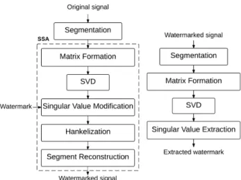
2.2 Embedding Process

The embedding process is shown in Fig. 4 (left). First, an audio signal is segmented into several non-overlapping frames.

To hide information, one bit of watermark is embedded into one frame. Therefore, frame length determines embedding capacity of a watermarking scheme. Then, a trajectory matrix representing a frame is constructed, and SVD is performed on the matrix. Information hiding is done by modifying singular values according to certain rule. Modifying of some singular values means physically that the amplitude of some oscillatory components are modified.

Fig. 2 Original and reconstructed signals (top). Residual signal or the diﬀerence between original and reconstructed signals (bottom).

(4)

Fig. 4 The embedding (left) and extraction (right) processes.

Fig. 5 Embedding “0” and “1” into the oscillatory componentX35.

Given a singular spectrum{√λ₁,√λ₂, . . . ,√λd}of an audio frame, a small number∈[0,0.5] and a watermark bit w∈ {0,1}, our proposed embedding rule can be summarized as follows.

λi=⎧⎪⎪⎨

⎪⎪⎩

√λl+(√λu−√λl), ifw=0

√λl+(1−)(√ λu−√

λl), ifw=1, (5) fori = u+1,u+2, . . . ,l−1, given that √λu is greater than

√λl.

Figure 3 shows an example of a singular spectrum and its modification after embedding “1” and “0”. Figure 5 shows an example of waveform when embedding “1” and

“0” into the oscillatory componentX35. 2.3 Extraction Process

The extraction process is shown in Fig. 4 (right). As in the embedding process, a watermarked signal is segmented into several non-overlapping frames, and each frame is mapped to a trajectory matrix. To extract singular values, SVD is used. The watermark bit is decoded by determining the me- dian, √λm, of{√λu+1,√λu+2, . . . ,√λl−1}. If √λmis closer to √

λuthan to √

λl, the watermark bit is 1. Otherwise, the watermark bit is 0.

3. Proposed Framework

The previously proposed framework showed its robustness against many attacks, and its objective evaluation of sound quality of a watermarked signal was very good, however,

Fig. 6 Diﬀerential evolution optimization.

when subjective tests were used for evaluation, some listen- ers could easily distinguish between some pairs of original and watermarked signals. Thus, the framework is in need of improvement. Two improvements have been done. The first one takes place in the singular-value-modification step, and the second one takes place in the singular-value-extraction step.

3.1 Diﬀerential Evolution-Based Singular Value Modifi- cation

The embedding rule described in Sect. 2.2 involves three important parameters,u,l, and. There is degradation in sound quality of a watermarked signal when a predefined and fixed parameter set {u,l, }is used. Since the singular spectrum varies from signal to signal, it is reasonable to set the parameters from the signal as well. Therefore, in order to reduce the distortion due to embedding, a new adaptive parameter set for each signal is required.

To solve such a problem while retaining robustness properly, differential evolution is used to find optimal parameters. Differential evolution is a parallel direct search method that optimizes the problem by iteratively improving candidate parameters with regard to a cost function. The following are reasons that differential evolution is select for this task. First, it is a multi-point optimizer, i.e., we can mitigate the effect of the starting point problem. Second, it is a derivative-free approach, i.e., we do not have to worry about whether the cost function is differentiable. Third, it has proved to be the fastest search algorithm in its computa- tional class[27].

The optimization deployed in the improved scheme is shown in Fig. 6. The cost function is defined as follows.

Cost=

α· LSD+

1−Sig

SDR²+β·BER², (6) where LSD, Sig(SDR), and BER are the log-spectral distance, the sigmoid function of signal-to-distortion ratio

(5)

(SDR) given that Sig(·) is a sigmoid function, and the average bit-error rate, respectively.

LSD is defined as the following formula. Given P(ω) and ˆP(ω) are power spectra of original and watermarked sig- nals respectively.

LSD=

1

2π π

−π

⎡⎢⎢⎢⎢⎢

⎣10 logP(ω) P(ω)ˆ

⎤⎥⎥⎥⎥⎥

⎦

2

dω (7)

SDR is the power ratio between a signal and the distortion. Given amplitudes of original and watermarked signals, A_sig(n) andA_syn(n), respectively, SDR is defined as follows.

SDR=10 log

n

[Asig(n)]²

n

[A_sig(n)−A_syn(n)]² (8) In short, the term LSD+(1−Sig(SDR)) in Eq. (6) represents a cost in terms of objective measures of inaudibility.

BER is the average of BER, number of error bits divided by the total number of embedded bits. Thus, it represents a cost in terms of robustness. Two user-defined con- stantsαandβwith relationshipα+β=1 control the balance of inaudibility and robustness, respectively. The diﬀerential evolution optimizer finds the parametersu,l, andthat min- imize the cost value. In our experiment, we set the parameters for diﬀerential evolution as follows: α=β=0.5, the maximum iteration is 20, and other constants, such as number of population and cross over constant are as suggested in[27]. Some constraints such as the minimum and maximum values ofuand the minimuml−uare set to reduce the search space.

3.2 Watermark-Bit Extraction by Polynomial Fitting According to the rule described in Sect. 2.2, the singular values √

λu+1 to √

λl−1 are replaced with the same value

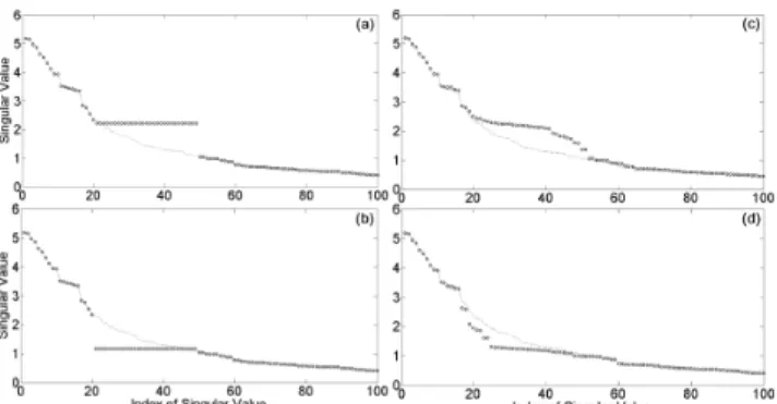
√λl+(√λu−√λl) or √λl+(1−)(√λu−√λl), depending upon the watermark bit. That is, in the embedding process, we force the singular spectrum on [u+1,l−1] to be flat, as shown in Figs. 7 (a) and (b). However, when all oscillatory components including the modified ones are combined to obtain a watermarked frame, the flatness resulting from rounding up or down of a sequence of singular value is dis- torted, as shown in Figs. 7 (c) and (d). The distortions form two patterns. When 0 is embedded, convexness of the singular spectrum is shown. On the other hand, if 1 is embedded, concave down of the singular spectrum is shown. We can use these characteristics to decode a watermark bit. In the extraction process of the previous framework, only the me- dian singular value is employed. To get a better result, the extraction rule is improved by using all information of modified singular values of [u+1,l−1].

The improved extraction method can be described as follows. Singular values of [u+1,l−1] are fitted to a degree- two polynomial,y(x)=ax²+bx+cwhereyis a singular

Fig. 7 Example of singular spectra in embedding and extraction processes: (a) when embedding “1” and (b) when embedding “0” in the embedding process, (c) singular spectrum of the frame embedded “1” and (d) singular spectrum of the frame embedded “0” in the extraction process.

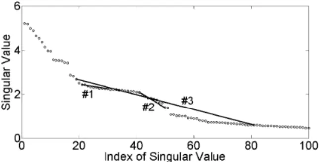
Fig. 8 The singular values of [18,32] are fitted to a quadratic equation y(x)=ax²+bx+c, wherea=−0.0146,b=0.598, andc=3.853. Since the value ofais negative, the graph is concave. Therefore, the watermark bit is 1.

value andxis the index of the singular value. The coeﬃcient aindicates the rate of change of singular values. Therefore, the sign of the coeﬃcientacan be used to decode a watermark bit: minus and plus signs indicate concavity or bit “1”

and “0”, respectively. An example of polynomial fitting is shown in Fig. 8, where a negative sign ofain the quadratic equation of the 18th–32rd singular values implies that the watermark bit “1” is embedded.

4. Automatic Parameter Estimation

The parameter set{u,l, }, obtained from diﬀerential evolution described in Sect. 3.1, is music-dependent. Our previous work[28]assumed that parametersu andlare known in the extraction process, and proposed using the second derivative of singular spectrum to automatically estimate them. However, further investigation shows that the proposed method works well only when u is the singular- value index selected somewhere in the singular spectrum where the slope changes rapidly. This paper proposes a new method for automatic parameter estimation. The extraction process with automatic parameter estimation is shown in Fig. 9.

Consider Fig. 10 for the basic concept of the parameter estimation method. A line segment of lengthn−mconnect- ing two singular values √λmand √λn is drawn, where m

(6)

Fig. 9 Extraction process with automatic parameter estimation.

Fig. 10 Singular spectrum of original signal and a line segment connecting√λ16and√λ37. Singular values on [17,36] are under the line segment.

Fig. 11 Singular spectrum of watermarked signal and two line segments.

Line segment #1 connects√λ16and √λ37, and line segment #2 connects

√λ21and√λ49. Into this frame, a watermark bit “1” is embedded by forc- ing √λ21to √λ49toward√λ20. The dotted curve represents the original singular spectrum. It can be seen that almost all of singular values are above the line segment #2.

andnare indices, andnis greater thanm. Note thatn−mis the length of its projection on the index axis. Naturally and statistically, a singular spectrum is convex upward. That is, givenmandn, most singular values of [m+1,n−1] are under the line segment. However, when a watermark bit “1” is embedded, for somemandn, there are some singular values above the line segment, as shown in Fig. 11. As a result, the number of singular values above given line segment can be used to detect the concave part of the singular spectrum.

This phenomenal can be used to estimate the parametersu andl.

Fig. 12 A line segment connecting √λ18and√λ42is used to calculate the concavity densityD18,42by summing up all diﬀerences between singular values and their associated values on the line segment from index 19 to index 41. D18,42in this example is−2.5353. The minus sign implies that the segment of the singular spectrum on [18,42] is convex.

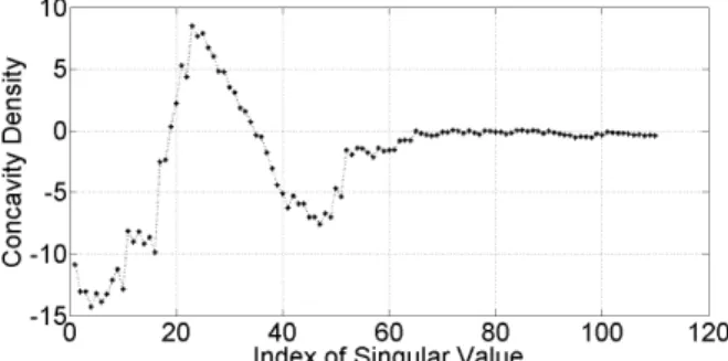
Fig. 13 A set of concavity density{D1,31,D2,32, . . . ,D110,140}. Notice that there is a strong relationship between regions of positive density and indices of modified singular values.

In this work, we define the concavity density as a measure of degree of concavity. Given a singular spectrum {√λ₁,√λ₂, . . . ,√λd}, the concavity densityDm,nof singular values from √

λmto√

λnis defined as follows.

Dm,n =

n−1

i=m+1

λi−L(i)

, (9)

whereL(i) is the function defining the line connecting √λm

and √λ_n. L(i)=

λm+

√λm−√λn

m−n

i−m

(10) Generally,Dm,n is the sum of subtraction between singular values and the line connecting √λ_m and √λ_n. An example of concavity density calculation is demonstrated in Fig. 12. Starting fromm=1, a line segment of length n−m, or a sequence of singular value that is used to calculate concavity density, is shifted to the right one singular- value point at a time to determine a set of concavity density {D1,n,D2,n+1, . . . ,Di,n+i−1, . . . ,Dd−n+1,d}. Figure 13 shows an example of concavity density curve of the singular spectrum in Fig. 11 when a line segment has a length of 30. It can be seen from this example that positive density corresponds roughly to the modification region of the singular spectrum.

Hence, it is possible that the parametersuandlcan be estimated by guidance from the concavity density. Fortunately,

(7)

the proposed extraction rules can decode a watermark bit without the parameter. We do not need to estimate it for the extraction process.

However, the concavity density depends upon the choice of the length of line segment, as shown in Fig. 14.

If the length is too short, such as line segments #1 and #2, or too long such as line segment #3, we may not be able to detect concavity. Figure 15 (a) shows concavity density curves with diﬀerent lengths. Therefore, in order to correctly estimate the parametersuandl, we have to choose an appro- priate length. In this work, we get around the problem by using the average density at diﬀerent lengths. The average density from Fig. 15 (a) is shown in Fig. 15 (b). To refine the density curve, we introduce a few constraints. First, a negative-density value is ignored because it implies convexness. Second, a positive-density curve that is narrower than

Fig. 14 The same singular spectrum as illustrated in Fig. 11 with three line segments. Line segment #1 connects √λ21and √λ30, and line segment #2 connects√λ41and √λ50. They are too short. We cannot detect the concavity of the singular spectrum on [21,30] and on [41,50] even though singular values on such intervals are modified to embed “1”. Line segment #3 connecting√λ19and √λ81is too long. It is diﬃcult to obtain the positive concavity density from long segments.

Fig. 15 (a) Concavity density curves when analyzing with four diﬀerent lengths. (b) An average of four curves in (a).

1.1·(l−u) is neglected because of the constraint on the min- imum value ofl−uin our diﬀerential evolution optimizer.

Then, the indices at rising and falling edges of a refined density curve, together with an oﬀsetting constant, are used to estimate the parametersuandlfor the given frame. Finally, the parametersuandlfor a music clip are calculated by av- eraging the estimated parametersuandlfrom all frames in the clip.

5. Evaluations

In our experiments, we implemented three models: fixed- parameter model and two adaptive-parameter models. The two adaptive-parameter models were partially-blind and completely-blind. The fixed-parameter model was based on the previously proposed framework[29], but it had a minor modification. That is, to increase robustness, one frame was divided into three equal subsegments where the same watermark bit was embedded repeatedly into those three subsegments, and the majority rule was applied in the extraction process. The extracted watermark bit of the frame is 1 if at least two-thirds of extracted watermark bits of its subsegments are 1; Otherwise, the extracted watermark bit of this frame is 0. Parameters for this model were set as follows.

Frame length was 7350, so that the embedding capacity was 6 bps. Sub-frame length Nwas 2450. The window length Lfor SSA was 500. Parametersu,l, andwere 20, 50, and 0.1, respectively.

Second, the partially-blind model was based on the proposed framework described in Sect. 3. This model was partially-blind because it assumed that the parametersuand lwere shared, somehow, between embedding and extraction processes. This model was similar to[28], but it also divided one frame into three equal subsegments and used the majority rule as well. The parameters determined by diﬀerential evolution are shown in Table 1.

Third, the completely-blind model was based on the proposed framework and automatic parameter estimation.

For the current implementation, the subsegment length was reduced to 816, instead of 2450, because when automatic parameter estimation was integrated into diﬀerential evolution optimization, the experiment was a time-consuming process. Since the less matrix dimension, the less computa- tional time, the size of a subsegment was reduced three times so that, in order to keep the capacity at about 6 bits per second, one frame was divided into nine equal subsegments.

The window length L for SSA was reduced to 326. The parameters determined by diﬀerential evolution are shown in Table 1. In automatic parameter estimation, five lengths were used: 15, 20, 25, 30, and 35.

Twelve host signals from the RWC music-genre database[30] (Track No. 01, 07, 13, 28, 37, 49, 54, 57, 64, 85, 91, and 100) were used in our experiments. All have a sampling rate of 44.1 kHz, 16-bit quantization, and two channels. A watermark was embedded in one channel at 6 bits per second. One hundred bits were embedded in total. Embedding duration was approximately 17 seconds.

(8)

Table 1 The parameters optimized by diﬀerential evolution as described in Sect. 3. and the number of iterations.

#01 #07 #13 #28 #37 #49 #54 #57 #64 #85 #91 #100

u 21 17 39 64 28 70 60 20 20 40 62 61

Partially-blind l 37 33 71 84 50 100 92 28 36 66 90 95

(The second model) 0.050 0.025 0.025 0.025 0.100 0.050 0.025 0.025 0.075 0.175 0.075 0.000

No. of iterations 11 11 11 10 11 11 11 12 11 13 11 9

u 74 60 84 92 83 100 53 50 89 56 75 66

Completely-blind l 134 108 144 152 141 154 107 92 145 104 125 114

(The third model) 0.000 0.025 0.025 0.000 0.000 0.000 0.000 0.075 0.025 0.000 0.000 0.000

No. of iterations 11 11 9 11 2 11 11 11 3 12 7 11

Table 2 ODGs, LSDs, and SDRs: comparison of the proposed models and the conventional method[7].

Fixed-parameter Partially-blind Completely-blind Conventional

PEAQ LSD SDR PEAQ LSD SDR PEAQ LSD SDR PEAQ LSD SDR

#01 0.20 0.21 19.86 0.21 0.13 26.28 0.21 0.18 28.44 0.20 0.08 26.50

#07 0.19 0.22 23.65 0.20 0.15 27.38 0.19 0.19 28.48 0.20 0.05 30.39

#13 0.20 0.11 25.35 0.20 0.09 29.84 0.20 0.10 30.52 0.20 0.05 29.71

#28 0.18 0.45 19.75 0.20 0.12 45.49 0.20 0.30 54.54 0.20 0.08 29.01

#37 0.19 0.27 31.04 0.20 0.13 39.50 0.20 0.21 47.79 0.20 0.07 29.19

#49 0.18 0.41 20.33 0.19 0.18 40.20 0.20 0.30 52.24 0.18 0.14 25.45

#54 0.19 0.27 20.60 0.20 0.14 34.14 0.19 0.18 27.88 0.20 0.10 25.68

#57 0.17 0.46 20.54 0.19 0.23 30.94 0.19 0.27 37.20 0.19 0.23 22.60

#64 0.18 0.23 25.45 0.20 0.13 30.93 0.21 0.18 38.17 0.20 0.06 31.08

#85 0.04 0.53 25.44 0.15 0.37 39.78 0.11 0.45 47.11 0.19 0.31 18.99

#91 0.19 0.35 20.24 0.20 0.13 38.65 0.19 0.29 43.30 0.20 0.07 29.00

#100 0.18 0.37 16.35 0.20 0.12 39.92 0.20 0.28 41.19 0.20 0.13 24.27

AV 0.18 0.32 22.38 0.19 0.16 35.25 0.18 0.24 39.74 0.20 0.11 26.82

SD 0.04 0.17 3.92 0.02 0.07 6.12 0.05 0.09 9.53 0.01 0.08 3.61

The first watermark bit was embedded starting from the ini- tial segment of host signals. We compared our proposed schemes with a conventional SVD-based scheme[7]. The scheme[7]was chosen as a reference for two reasons: it is one of a few blind SVD-based techniques, and its published results are promising.

5.1 Sound-Quality Tests

To evaluate the sound quality of a watermarked signal, objective and subjective tests were conducted. For objective evaluation, three evaluations: the perceptual evaluation of audio quality (PEAQ), LSD, and SDR were used. PEAQ measures the degradation of the watermarked signal being evaluated, compared with the original and covers a scale, called objective diﬀerence grade (ODG), from−4 (worst) to 0 (best). LSD is a distance measure between two spectra, as defined in Eq. (7). SDR is the power ratio between the signal and the distortion, as defined in Eq. (8).

We also verify the perfection of SSA as an analysis- synthesis tool by checking the ODG, LSD, and SDR of synthesis signals, compared to the originals. The results showed that all ODGs were positive, all LSDs were zero, and all SDRs were infinity[29]. In other words, the framework of singular-spectrum analysis is perfect in the sense that the framework itself does not introduce noise into the system.

5.1.1 Objective Evaluation

The ODG, LSD, and SDR of a watermarked signal, compared between the proposed and conventional schemes, are shown in Table 2. The results show that ODGs from all schemes are at the same level. However, LSDs from adaptive-parameter models drop considerably from 0.32 to 0.16, and to 0.24 for partially-blind and completely-blind models, respectively. SDRs from adaptive-parameter models increase significantly as well, i.e., from 22.38 dB to 35.25 dB, and to 39.74 dB. Therefore, the sound quality of a watermarked signal improves.

5.1.2 Subjective Evaluation

The ABX test was used to evaluate sound quality of a watermarked signal, subjectively. It is a method of comparing two choices to identify whether a listener can perceive a diﬀer- ence between them or not. First, we presented a subject with two clips, A and B, and then, after presenting the third clip X, which is randomly selected from either A or B, we asked the subject to identify X as either A or B. In our experiment, A was the original signal, and B was the watermarked signal. The sequence of presenting A and B to participants was random. We tested 20 audio clips in total. There were 35

(9)

normal-hearing subjects involved in the test. We assumed a binomial distribution and used it as a statistical analysis tool. Typically, the 95% confidence level is suﬃcient for psychoacoustic experiments, i.e., to reach such a level, 14 out of 20 correct identifications was the criterion indicating a perceptible diﬀerence. The results are shown in Table 3.

As a result, the partially-blind model outperformed the fixed-parameter model, and we can say that the diﬀerence in sound quality between the original and watermarked signals obtained from our scheme was almost imperceptible because the average correct identification from the ABX test was at the chance level.

In this experiment, we examined only the fixed- parameter model and the partially-blind model. We did not subjectively evaluate the completely-blind one. However, we expect that the completely-blind model will work well because of two reasons. First, all objective scores from the completely-blind model were comparable to those from the partially-blind model. Second, the singular values, which

Table 3 The average, maximum, and minimum correct identification of the ABX tasks with 20 stimuli for the fixed-parameter and partially-blind, adaptive-parameter models.

Fixed Adaptive Average correct identification (%) 73.00 49.78 Maximum correct identification 19 13 Minimum correct identification 9 7

Table 4 BER (%) comparison of fixed-parameter (Fix.), partially-blind (Par.), completely-blind (Com.), and conventional (Con.) methods when attacks (MP3, MP4, AWGN, Re-sampling, and Band- pass filtering) were performed.

#01 #07 #13 #28 #37 #49 #54 #57 #64 #85 #91 #100 AV SD

Fix. 0.00 0.33 0.08 0.00 0.00 0.00 0.18 0.51 0.02 0.00 0.18 0.02 0.11 0.16

No Attack Par. 0.00 0.02 0.02 0.00 0.00 0.02 0.08 0.98 0.02 0.18 0.02 0.02 0.11 0.28

Com. 0.00 0.00 0.00 0.00 0.03 0.00 0.00 0.00 0.00 0.00 0.00 0.06 0.01 0.02

Con. 0.00 0.00 0.00 0.00 0.00 0.00 0.00 0.00 0.00 0.00 0.00 0.00 0.00 0.00

Fix. 0.08 0.51 12.05 0.00 0.18 0.02 0.98 0.51 0.18 0.00 0.73 0.08 1.28 3.41

MP3 Attack Par. 0.00 0.18 6.08 0.33 0.33 0.18 1.97 0.73 0.08 1.27 2.37 0.51 1.17 1.72

Com. 4.64 5.16 5.71 9.88 11.60 9.08 6.31 6.94 18.90 1.06 4.16 18.90 8.53 5.59

Con. 47.22 98.33 70.56 87.78 82.50 33.06 41.94 33.61 95.83 18.89 74.72 23.61 59.00 29.03

Fix. 0.00 0.33 0.08 0.00 0.00 0.00 0.18 0.51 0.02 0.00 0.18 0.02 0.11 0.16

AWGN Par. 0.00 0.02 0.02 0.00 0.00 0.02 0.08 0.98 0.02 0.18 0.02 0.02 0.11 0.28

Com. 0.00 0.00 0.00 0.00 0.03 0.00 0.00 0.00 0.00 0.00 0.00 0.06 0.01 0.02

Con. 0.00 0.00 0.00 0.00 0.00 0.00 0.00 0.00 0.00 0.00 0.00 0.00 0.00 0.00

Fix. 0.00 0.51 6.08 0.00 0.08 0.00 0.33 0.98 0.08 0.00 0.51 0.00 0.71 1.72

MP4 Attack Par. 0.18 0.18 17.54 0.51 0.18 0.00 4.30 2.80 0.33 0.51 3.27 1.97 2.65 4.91

Com. 26.66 7.62 25.28 28.07 41.85 41.85 6.31 12.52 20.11 3.29 25.28 40.24 23.25 13.74

Con. 0.28 0.00 13.89 0.00 0.00 0.00 0.00 0.00 0.00 0.00 0.00 0.28 1.20 4.00

Fix. 0.01 0.41 7.41 0.00 0.18 0.00 0.13 0.25 0.05 0.00 0.08 0.05 0.71 2.11

Re-sampling Par. 0.05 0.02 9.61 0.01 0.25 0.02 0.33 1.78 0.05 0.25 0.61 0.13 1.09 2.73

Com. 53.68 1.32 36.50 36.04 38.20 32.53 0.55 1.46 36.14 0.03 25.83 45.30 25.63 19.48

Con. 3.19 0.42 25.69 0.00 0.00 0.00 0.00 0.00 0.28 0.83 0.14 1.53 2.67 7.31

Fix. 0.08 0.51 30.47 0.02 0.73 0.00 0.51 2.80 0.18 0.02 0.98 0.02 3.03 8.68

BP Filtering Par. 0.73 0.08 35.20 0.18 0.73 0.18 3.27 15.63 0.33 0.18 6.08 0.98 5.30 10.43 Com. 53.28 17.74 59.76 59.76 50.00 54.91 4.16 4.16 67.54 0.62 20.11 51.64 36.97 25.36 Con. 25.83 48.61 47.78 43.61 56.67 21.39 40.56 28.89 62.22 0.83 50.56 30.00 38.08 17.30

were modified by the completely-blind model, were much smaller than those by the partially-blind model, as shown in Table 1. Note that the detection method relates to the results of the objective or subjective evaluations because in the embedding process, the detection process is simu- lated by the diﬀerential evolution optimization, as shown in Fig. 6. Hence, this aﬀects optimized parameters and the sound quality.

5.2 Robustness Tests

Five attacks were performed on watermarked signals:

Gaussian-noise addition with average SNR of 36 dB, re- sampling with 16 and 22.05 kHz, band-pass filtering with 100–6000 Hz and−12 dB/Oct, MP3 compression with 128 kbps joint stereo, and MP4 compression with 96 kbps.

We represent extraction precision in terms of bit error rate (BER), and the BER should be lower than 10%.

The results of robustness tests are shown in Table 4.

BERs from the proposed and conventional SVD-based schemes were compared. The average BERs of fixed parameter model, partially-blind model, and completely-blind model were 0.99%, 1.74%, and 15.73% respectively. The average BER of conventional method was 16.83%. There- fore, the fixed-parameter and partially-blind models outperformed the conventional SVD-based method in robustness.

Because the average BER from the partially-blind models increased, compared with the fixed-parameter

(10)

model, we can consider the results as a trade-oﬀbetween inaudibility and robustness. However, it is not linear. While the robustness drops very little (i.e., BER increased from 0.99% to 1.74%), the inaudibility improves considerably (i.e., the average correct identification dropped to chance level, and all objective scores were better).

When no attack was performed, the BER from the completely-blind model was the best, compared with the other two proposed models. Since a watermark bit is extracted by the polynomial fitting as described in Sect. 3.2, the BER is highly dependent on the value ofu −l. The greater the value, the easier, extracting the watermark bit.

The values ofu−lin the completely-blind model are greater than those in the other two models. Therefore, it is more robust under no-attack. However, it was the most fragile if it was under attacks except for added 36 dB noise and MP3 compression. The fragility to signal processing of this model is discussed in the next section.

6. Discussion

All three models that we proposed have their own advantages and disadvantages. The fixed-parameter model is sim- plest and does not involve in any music-dependent parameters. Thus, it can extract hidden information completely blindly. It is robust. The average BER is just 0.0099 or 0.9919%. However, for some stimuli, distortion in sound quality occurs. This problem can be resolved by incorporating diﬀerential evolution into the SSA-based framework in order to determine optimal parameters. If we can share these parameters between the embedding and extraction processes, the partially-blind model satisfies inaudibility and robustness, simultaneously. The third, completely- blind model was proposed for a scenario in which sharing parameters is not allowed. Hence, the extraction process must be able to estimate the parameters by analyzing watermarked signal, only. Without attacks, this model works well with the average BER of 0.000087, or 0.0087%. Its fragility to signal processing can be explained after con- sidering Table 1. The modification region [u,l] suggested by diﬀerential evolution for the completely-blind model is much lower than that for the partially-blind model. As discussed in Sect. 2.1.4, the smaller the singular value, the less contribution to the signal. Thus, the oscillatory component associated with a small singular value is easily damaged.

There are two factors that may account for the reason the differential evolution optimization suggested those parameters. The first one is that the optimization in Fig. 6 is too simplistic because it includes only the MP3 compression simulation. In fact, it should include as many attacks as possible. The second factor involves the concavity density function since the optimization simulates the extraction process as illustrated in Fig. 9, i.e., the automatic parameter estimation affects the optimization significantly. Thus, es- timating parameters with different methods could result in different sets of optimal parameters.

However, the current completely-blind model is suit-

able in the application in that robustness against intentional attack is not required, such as an information carrier application[31].

Under no-attack, AWGN-attack, and MP4-attack, the conventional method shows the best performance. Its robustness when there is no attack is due to the characteristics of dither-modulation quantization[7]. According to the extraction rule of the conventional method, which deploys the Euclidean norm and a predefined quantization step to decode a watermark bit, robustness can be expected if the singular values obtained from a watermarked frame are not much diﬀerent from those after an attack to the frame. We found that this condition is true when AWGN and MP4 are applied to a watermarked frame. Therefore, the conventional method is very robust against AWGN and MP4.

There are two important issues concerning the scope of this work we would like to discuss in this section as well.

First, since the completely-blind model can decode a watermark blindly, one can analyze the singular spectrum of a watermarked frame in order to extract the watermark bit.

Therefore, confidentiality of the hidden bit seems reduced once an attacker knows the frame position. This problem may be solved by combining encryption techniques with the proposed SSA-based framework. That is, the watermark information is encrypted before embedding. However, there is another problem, i.e., if an attacker analyzes the singular spectrum in a similar way as the automatic parameter estimation does, then the attacker can intentionally attack the hidden bit by modifying singular values on some specific ranges. This issue will be investigated further in our future work.

Second, we assume the extraction process knows exactly where the frame position is. The frame synchronization is beyond the scope of this work. As suggested in[24], there are two ways to solve the synchronization problem:

binding the watermark with invariant audio features and using synchronization code, such as a chaotic map[32]. We will solve this problem as the next issue in our framework.

7. Conclusion

This paper presents the deployment of SSA for digital audio watermarking and proposes an audio watermarking framework based on it. From our experiment, we discover that it does not introduce noise into the reconstructed signal. We improved the inaudibility property of the result by using differential evolution to find optimal parameters. Furthermore, based on analyzing singular spectrum with concavity density function, the parameters can be estimated automatically.

We present three models and show their advantages and disadvantages. The fixed-parameter model and the partially- blind model are robust against many attacks, especially MP3 and MP4 compression, and the adaptive-parameter models satisfy inaudibility subjectively and objectively.

(11)

Acknowledgments

This work was supported by a Grant-in-Aid for Scientific Research (B) (No. 23300070) and A3 foresight program made available by the Japan Society for the Promotion of Science. It was also under a grant in the SIIT-JAIST- NECTEC Dual Doctoral Degree Program.

References

[1] T. Dutoit and F. Marqu´es, Applied Signal Processing: A MATLAB^TM-Based Proof of Concept, Springer, 2009.

[2] S.A. Craver, M. Wu, and B. Liu, “What can we reasonably expect from watermarks?,” Proc. IEEE Workshop on Application of Signal Processing to Audio and Acoustics, pp.223–226, 2001.

[3] M. Unoki and R. Miyauchi, “Method of digital-audio watermarking based on Cochlear delay characteristics,” K. Kondo (ed.), Multime- dia Information Hiding Technologies and Methodologies for Con- trolling Data, pp.42–70, Information Science Reference, 2013.

[4] M. Fallahpour and D. Meg´ıas, “High capacity audio watermarking using the high frequency band of the wavelet domain,” Multimedia Tools and Applications, vol.52, no.2-3, pp.485–498, 2011.

[5] E. Erc¸elebi and L. Batakc¸ı, “Audio watermarking scheme based on embedding strategy in low frequency components with a binary im- age,” Digital Signal Processing, vol.19, no.2, pp.265–277, 2009.

[6] M. Unoki and D. Hamada, “Method of digital-audio watermarking based on cochlear delay characteristics,” International Journal of In- novative Computing, Information and Control, vol.6, no.3, pp.1325–

1346, 2010.

[7] V. Bhat K, I. Sengupta, and A. Das, “A new audio watermarking scheme based on singular value decomposition and quantization,”

Circuits, Systems and Signal Processing, vol.30, no.5, pp.915–927, 2011.

[8] V. Bhat K, I. Sengupta, and A. Das, “An audio watermarking scheme using singular value decomposition and dither-modulation quantization,” Multimedia Tools and Applications, vol.52, no.2-3, pp.369–383, 2011.

[9] H. ¨Ozer, B. Sankur, and N. Memon, “An SVD-based audio watermarking technique,” Proc. 7th Workshop on Multimedia and Secu- rity, pp.51–56, 2005.

[10] L. Lamarche, Y. Liu, and J. Zhao, “Flaw in SVD-based watermarking,” Proc. Canadian Conference on Electrical and Computer Engi- neering, pp.2082–2085, 2006.

[11] F.E.A. El-Samie, “An eﬃcient singular value decomposition algorithm for digital audio watermarking,” International Journal of Speech Technology, vol.12, no.1, pp.27–45, 2009.

[12] A. Al-Haj, C. Twal, and A. Mohammad, “Hybrid DWT-SVD audio watermarking,” Proc. 5th International Conference on Digital Infor- mation Management, pp.525–529, 2010.

[13] S. Vongpraphip and M. Ketcham, “An intelligence audio watermarking based on DWT-SVD using ATS,” Proc. WRI Global Conference on Intelligence Systems, pp.150–154, 2009.

[14] A. Al-Haj and A. Mohammad, “Digital audio watermarking based on the discrete wavelets transform and singular value decomposition,” European Journal of Scientific Research, vol.39, no.1, pp.6–

21, 2010.

[15] M.S. Al-Yaman, M.A. Al-Taee, and H.A. Alshammas, “Audio watermarking based ownership verification system using enhanced DWT-SVD technique,” Proc. International Multi-Conference on Systems, Signals and Devices, pp.1–5, 2012.

[16] J. Zhang, “Analysis on audio watermarking algorithm based on SVD,” Proc. 2nd International Conference on Computer Science and Network Technology, pp.1986–1989, 2012.

[17] A. Singhal, A.N. Chaubey, and C. Prakkash, “Audio watermarking

using combination of multilevel wavelet decomposition, DCT and SVD,” Proc. International Conference on Emerging Trends in Net- works and Computer Communications, pp.239–243, 2011.

[18] P.K. Dhar and T. Shimamura, “Audio watermarking in transform domain based on singular value decomposition and quantization,” Proc. 18th Asia-Pacific Conference on Communications, pp.516–521, 2012.

[19] P.K Dhar and T. Shimamura, “An audio watermarking scheme using discrete Fourier transformation and singular value decomposition,” Proc. 35th International Conference on Telecommunications and Signal Processing, pp.789–794, 2012.

[20] P.K Dhar and T. Shimamura, “A DWT-DCT-based audio watermarking method using singular value decomposition and quantization,”

Journal of Signal Processing, vol.17, no.3, pp.69–79, 2013.

[21] G. Suresh, N.V. Lalitha, C.S. Rao, and V. Sailaja, “An eﬃcient and simple audio watermarking using DCT-SVD,” Proc. International Conference on Devices, Circuits and Systems, pp.177–181, 2012.

[22] S. Karimimehr, S. Samavi, H.R. Kaviani, and M. Mahdavi, “Robust audio water-marking based on HWD and SVD,” Proc. 20th Iranian Conference on Electrical Engineering, pp.1363–1367, 2012.

[23] W.-Z. Jiang, “Fragile audio watermarking algorithm based on SVD and DWT,” Proc. International Conference on Intelligent Computing and Integrated Systems, pp.83–86, 2010.

[24] B. Lei, I.Y. Soon, and E.-L. Tan, “Robust SVD-based audio watermarking scheme with diﬀerential evolution optimization,”

IEEE Trans. Audio, Speech, Language Process., vol.21, no.11, pp.2368–2378, 2013.

[25] N. Golyandina, V. Nekrutkin, and A. Zhigljavsky, Analysis of Time Series Structure: SSA and related techniques, Chapman and Hall/CRC, 2001.

[26] H. Hassani, “Singular spectrum analysis: Methodology and comparison,” Journal of Data Science, vol.5, no.2, pp.239–257, 2007.

[27] R. Storn and K. Price, “Diﬀerential evolution — A simple and eﬃ- cient heuristic for global optimization over continuous spaces,” Jour- nal of Global Optimization, vol.11, no.4, pp.341–359, 1977.

[28] J. Karnjana, P. Aimmanee, M. Unoki, and C. Wutiwiwatchai,

“An audio watermarking scheme based on automatic parameterized singular-spectrum analysis using diﬀerential evolution,” Proc. Asia- Pacific Signal and Information Processing Association Annual Sum- mit and Conference, pp.543–551, 2015.

[29] J. Karnjana, M. Unoki, P. Aimmanee, and C. Wutiwiwatchai, “An audio watermarking scheme based on singular-spectrum analysis,”

Digital-Forensics and Watermarking, Lecture Notes in Computer Science, vol.9023, pp.145–159, Springer International Publishing, Cham, 2015.

[30] RWC database: https://staﬀ.aist.go.jp/m.goto/RWC-MDB/ [Ac- cessed 25 April 2016]

[31] N. Cvejic and T. Sepp¨anen, Digital Audio Watermarking Techniques and Technologies: Applications and Benchmarks, IGI Global, 2007.

[32] S. Wu, J. Huang, D. Huang, and Y.Q. Shi, “Eﬃciently self- synchronized audio watermarking for assured audio data transmis- sion,” IEEE Trans. Broadcast., vol.51, no.1, pp.69–76, 2005.