Childcare Policy and Regional Employment of Japanese Female Workers

(1)

Panel Data Research Center at Keio University

DISCUSSION PAPER SERIES

DP2014-008 March, 2015

Isamu Yamamoto＊

Hirotaka Ito＊

【Abstract】

This paper conducts the evaluation of the childcare policy, “General Childcare-Support for Model-municipalities,” which was implemented for target model regions in Japan in the 2000s. We employ the difference-in-differences methods based on regression model and propensity score matching, to examine changes in women’s employment and working hours in the target model regions before and after the policy’s implementation. The estimation results imply that there has been an increase in the non-regular workers living in the target model regions of the policy, particularly among those working voluntarily as non-regular employees. This tendency is especially prominent among married women who graduated from junior/technical college, or who care for many children under the age of six years. There is also the possibility that the program has prompted an increase in the working hours of regular workers. However, as these influences are not confirmed after controlling for the regional factors such as financial index, we interpret that the effects on the employment of married women are caused not by the designation of “model region” by the government, but rather by the active childcare supports provided by municipalities.

＊_{Graduate School of Business and Commerce, Keio University}

(2)

Childcare Policy and Regional Employment

of Japanese Female Workers

∗

Isamu Yamamoto* _{Hirotaka Ito}

Keio University Keio University

Abstract

This paper conducts the evaluation of the childcare policy, “General Childcare-Support for Model-municipalities,” which was implemented for target model regions in Japan in the 2000s. We employ the difference-in-differences methods based on regression model and propensity score matching, to examine changes in women’s employment and working hours in the target model regions before and after the policy’s implementation. The estimation results imply that there has been an increase in the non-regular workers living in the target model regions of the policy, particularly among those working voluntarily as non-regular employees. This tendency is especially prominent among married women who graduated from junior/technical college, or who care for many children under the age of six years. There is also the possibility that the program has prompted an increase in the working hours of regular workers. However, as these influences are not confirmed after controlling for the regional factors such as financial index, we interpret that the effects on the employment of married women are caused not by the designation of “model region” by the government, but rather by the active childcare supports provided by municipalities.

Keywords: Female employment, Propensity score matching, Difference-in-Differences analysis, Childcare support

* Corresponding Author: [email protected], Tel/Fax: +81-3-5427-1085

∗_{The authors deeply appreciate Yoshio Higuchi, Michio Naoi, and Yasuhiro Nohara for their}

valuable comments. We are grateful for access to the micro data from the “Keio Household Panel Survey,” provided by the Panel Data Research Center at Keio University. Any remaining errors are entirely our own.

(3)

1. Introduction

Utilization of the female workforce is an important issue in Japan, given that country’s aging population and low birth rates. As of 2010, labor force participation ratio of women aged 25–29 is 77.1% in Japan, 75.6% in the United States, and 77.8% in the United Kingdom, which indicates no major differences among the three countries. The ratio for women aged 35–39 years, however, is extremely low in Japan (66.2%), compared to 74.1% in the United States and 76.4% in the United Kingdom. For women aged 45–49 years, the Japanese female workforce ratio increases to 75.8%, a level almost the same as that in the United States (76.8%) and the United Kingdom (82.2%); however, in Japan, approximately 60% of the female workforce in this age range are employed as non-regular workers1_{. These} trends constitute the so-called M-shaped curve for Japanese women, as Japanese female workers tend to retire from the labor market once they reach their 30s and then reenter the labor market in their 40s as non-regular employees.

Considering the fact that the mean age of women at their first child’s live birth is 30.3 years,2_{we can point out that the difficulty of maintaining balance} between child-rearing and work in the Japanese labor market could be one of the reasons for the decline in the participation ratio among women in their 30s. Thus, it should be important to explore the effective measures taken by companies and governments to create a system or an environment by which women can balance child-rearing and work.

1_{The data are based on the “Databook of International Labour Statistics” (Japan Institute for}

Labour Policy and Training, 2012) and the “Labour Force Survey” (Ministry of Internal Affairs and Communications, 2013).

2_{The data is based on the “Vital Statistics in Japan 2014 (Trends up to 2012)” (the Ministry of}

Health, Labour and Welfare).

(4)

Typical examples of company-based child-rearing support measures include the parental leave system, the short working hour system, and other work–life balance measures. Due to a recent increase in interest in work–life balance, the provision of work environments friendly to women is under way, and empirical studies have examined the relationship between company-based work–life balance measures and female workforce utilization in companies. For example, Suruga and Zhang [2003] finds that companies where parental leave systems have been explicitly stipulated have seen an increase in the share of women employment. Kawaguchi [2011] provides an evidence that companies where work–life balance measures have been developed have a higher ratio of female employment. Examining the factors to enforce female workforce utilization in companies, Yamamoto [2014] shows that more female workers are being utilized as regular workers among companies introducing well-developed work–life balance measures or exhibiting shorter working hours.3_{Based on the findings of these studies, it is highly likely that} company-based child-rearing support and work–life balance measures help promote female workforce utilization.

On the other hand, not many studies have been conducted with regard to the effects of child-rearing support measures in the public sectors, especially the municipalities, and those studies have mixed results. As a national policy to overcome the declining birthrate, the government established the “Act for Measures to Support the Development of the Next Generation” in 2003; since then, many child-rearing support measures—such as the “regional childcare support center program” and the “Child and Child-Rearing Support Plan”—have been formulated. At the same time, municipalities and local governments have been implementing a

3_{In addition to these studies, studies on support measures for maintaining work–life balance and}

women’s employment include Higuchi [1994], Tomita [1994], Morita and Kaneko [1988], and Matsushige and Takeuchi [2008], among others.

(5)

variety of measures, including expansions in the capacity of daycare centers, as part of government programs like the “General Childcare-Support for Model-municipalities” or as part of their own measures.

The “General Childcare-Support for Model-municipalities” is a child-rearing support measure that was established by the government in 2004; 50 municipalities in Japan were designated as targets under this program, which sought to provide government support to the comprehensive and active child-rearing support systems offered by the local governments. However, previous studies in Japan have not conducted an analysis of policy evaluation for the government programs in specific target model regions or regional child-rearing support measures on women’s employment. Additionally, we find the mixed results in the previous studies that examined the effect of daycare centers on the female workforce.

For example, Ohishi [2003] points out that expanding the availability of daycare centers increases the probability of employment among mothers, and Maruyama [2001] asserts that there is a strong tendency for working women to demand the expansion of childcare services. Higuchi, Matsuura, and Sato [2007], on the other hand, shows that the expansion of childcare services does not always have a positive effect on women’s employment.

Therefore, this paper examines the effect of the “General Childcare-Support for Model-municipalities” on women’s employment in Japan, based on the framework of policy evaluation analysis. Specifically, we use individual-level panel data collected through the “Keio Household Panel Survey” (KHPS), which covers households across Japan, to examine whether the employment rate among women increased in the target model regions following the implementation of this policy; we do so by conducting difference-in-differences (DD) analysis.

(6)

tendency of increase in the non-regular employment of married women— particularly in voluntary non-regular employment—in the target model regions (municipalities) due to the implementation of the “General Childcare-Support for Model-municipalities.” This tendency is prominent for junior college/technical college graduates, and for married women with many children under the age of six years. We also find that this program increased the working hours of women who work as regular employees. Focusing on the program’s structure in which the government designates the “model regions (municipalities)” where the plan for the child-rearing support measures is active and comprehensive, we then identified whether the effects on women’s employment were produced by the efforts made by the municipalities or by the government’s “model region” designation. Our findings imply that it is highly likely that the increase in the non-regular employment rate among women was caused not by the “model region” designation but by the efforts made by the municipalities.

The structure of this paper is as follows. Section 2 provides an overview of the “General Childcare-Support for Model-municipalities,” and introduces previous studies on similar policies. Following this, Section 3 explains the estimation framework, data, and variables used in this study. Section 4 outlines changes in the employment rate of women in the model and non-model regions; it also provides the estimation results of DD analysis. Finally, Section 5 summarizes the estimation results and the implications.

2. General Childcare-Support for Model-municipalities

(7)

of the Japanese government; it was established in 2004 with the aim of “contribut[ing] to the promotion of national programs for child-rearing support by designating approximately 50 municipalities where comprehensive and active measures are implemented for various child-rearing support services under the municipality action plan formulated by the end of FY 2004.”4_{Model regions covered} by the policy were selected based on the contents of their municipality action plan for child-rearing for the first half of the term (2005–09), which was created in accordance with the requirements of 2003’s “Act for Measures to Support the Development of the Next Generation.”5_{Specifically, the structure of the program} allowed for the designation of those municipalities whose mandatory programs and optional programs specific to child-rearing supports under the municipality’s action plan for the first half of the term6_{were considered excellent, as “model regions.” As} such, under the program, regions with active child-rearing support measures were selected. Support measures—such as subsidies for the costs related to the formulation of model program promotion plans—were implemented among the selected “model region” municipalities.

Many of the government’s past child-rearing policies offered the same service contents to all regions, and the particulars of policy operations were left to each of the municipalities themselves. In contrast, the “General Childcare-Support for Model-municipalities” featured a structure that called for the selection of municipalities with comprehensive and active action policies, and it designated

4 _{This is excerpted from the website of Ministry of Health, Labour and Welfare}

(http://www.mhlw.go.jp/houdou/2004/06/h0618-6b.html).

5_{Refer to http://www.mhlw.go.jp/houdou/2004/06/h0618-6a.html for details.}

6_{Mandatory programs include short-time daycare support programs, home child-rearing support}

programs, child-rearing counseling support programs, and child-rearing support comprehensive coordination programs, while optional programs include short-term child-rearing support programs, home-visiting temporary daycare programs, and specific daycare programs.

(8)

those limited regions as targets of the model programs. In this sense, we consider this program to be different from previous ones, and so analysis of its effects is important.

On the other hand, the results of policy evaluation of this program must be interpreted carefully. This is because the program designated specific regions as model regions, and at the time of designation, the model regions had already formulated comprehensive and active action plans by which to provide child-rearing support. Therefore, even if the increase of employment rate among the parenting-age women within the model regions of this program was higher than that in other regions, both of the following effects could be interpreted as having taken place: (1) the effects of the action plan and measures that were originally formulated by the municipalities, and (2) additional effects produced by being designated as a model region.

It is important to identify how municipality action plan and child-rearing support service contents affect the balancing of childcare and work for women. At the same time, it is also important to confirm whether the model programs and other government measures have been effective. Accordingly, in this paper, we measure the effects of combining these programs and measures, and also identify any additional effects that stem from a “model program” designation by the government, by controlling for the financial state of each municipality and the variables that can affect the efficacy of child-rearing support measures.

Note, as mentioned, model regions under the “General Childcare-Support for Model-municipalities” were designated based on their action plan for the first half of the term (2005–09) under the “Act for Measures to Support the Development of the Next Generation”; however, municipalities continued to provide child-rearing support services in the latter half of the term (2010–14). Therefore, we assume the

(9)

possibility that the effects of the “General Childcare-Support for Model-municipalities” could persist beyond the end of the program period—or from 2010 onwards, when municipality measures continued, based on the action plan for the term’s latter half. In any case, that later plan naturally followed the action plan for the term’s first half.

As described in the previous section, no studies on Japan’s “General Childcare-Support for Model-municipalities” have been conducted; however, several studies have examined the effect of similar child-rearing policies implemented in Canada, for which specific target regions were designated. Under the child-rearing support policy in Canada, daycare space is provided for children under the age of four, at reduced prices; this policy has been in place since 1997, but only in the province of Quebec.

Lefebvre and Merrigan [2008] conduct empirical studies to estimate the effects of this policy on women’s employment by conducting DD analysis, wherein the province of Quebec was set as the treatment group and the other provinces as the control group; their analytical results show that the policy had indeed increased the female labor supply in Quebec. Furthermore, Lefebvre, Merrigan, and Verstraete [2009] conduct detailed analysis of the child-rearing support policy in Quebec and find that the policy had a substantial effect, especially among women with low levels of education attainment. Other than these studies, Baker, Gruber, and Milligan [2008] derive similar results, that the child-rearing support policy in Quebec increased the female labor supply there.

Similar to these studies, we undertake a policy evaluation analysis of the “General Childcare-Support for Model-municipalities” by implementing DD analysis, wherein we set the policy target model regions as the treatment group and the other regions as the control group.

(10)

3. Analytical Approach

3.1 Estimation model

To estimate the influence of the “model region” designation on women’s employment, we define the women living in municipalities designated as model regions under the “General Childcare-Support for Model-municipalities” as the treatment group, and the women living in the other municipalities as the control group. To confirm the robustness, we conduct two sets of DD analysis, the one using a regression and the one using a propensity score matching.

In the DD analysis using a regression model, we estimate the equation (1) as a random-effect probit model, a random-effect linear model, or a fixed-effect linear model, according to the dependent variables:

𝑌𝑌𝑖𝑖𝑖𝑖 = 𝑀𝑀𝑖𝑖∙ 𝑻𝑻𝒕𝒕𝜷𝜷𝟏𝟏+ 𝛽𝛽2𝑀𝑀𝑖𝑖 + 𝑻𝑻𝒕𝒕𝜷𝜷𝟑𝟑+ 𝑿𝑿𝑖𝑖𝜷𝜷4+ 𝐹𝐹𝑖𝑖+ 𝜀𝜀𝑖𝑖𝑖𝑖, (1)

where 𝑌𝑌𝑖𝑖𝑖𝑖 represents dependent variables showing the status of individual 𝑖𝑖 in the

year 𝑡𝑡, with or without employment, regular employment, non-regular employment, or voluntary non-regular employment, or the average weekly working hours. 𝑀𝑀𝑖𝑖 is

a dummy variable indicating a model region (or treatment group); 𝑻𝑻𝒕𝒕 is a vector

of year dummy variables; 𝑿𝑿𝒕𝒕 is a vector of control variables including academic

background, home environment, and other individual attributes; 𝐹𝐹𝑖𝑖 is a

time-invariant individual effect; and 𝜀𝜀𝑖𝑖𝑖𝑖 is an error term.

As described above, the “General Childcare-Support for Model-municipalities” was initiated as a policy in the 2004 fiscal year, based on the action plan for the first half-term (2005–09). However, municipalities naturally also had long-term measures in the latter half of the term (2010–14). Therefore, we take into

(11)

account the possibility of a time lag for the effects of the model programs or the child-rearing support policy of municipalities. Specifically, data from before the policy was initiated in 20047_{and up to 2012 are used to set the time-based} comparison points at three-year intervals: the period 2004-06, 2007-09, and 2010-12. Thereafter, year dummy variables which take the value of 1 for the period 2007-09 and that for 2010-12 are included in 𝑇𝑇𝑖𝑖, by setting the period 2004-06 as a base

when the policy effect was not evident. Therefore, the coefficient 𝜷𝜷𝟏𝟏 of the

cross-terms of the model region dummy and the year dummies represents the average treatment effect (ATE) of the child-rearing policy in which this study has an interest.

In the DD analysis using propensity score matching, we match individuals with similar attributes based on the propensity score. First, we use the probit model of equation (2), to regress the probability of belonging to the treatment group (i.e., propensity score) with individual attributes.

𝑒𝑒𝑖𝑖 = Pr(𝑀𝑀𝑖𝑖 = 1|𝑿𝑿𝑖𝑖) = 𝐸𝐸(𝑀𝑀𝑖𝑖|𝑿𝑿𝒊𝒊) (2)

In equation (2), 𝑒𝑒𝑖𝑖 indicates the probability of belonging to the treatment group

given individual attributes 𝑿𝑿𝒊𝒊. Using the estimated propensity score 𝑒𝑒𝑖𝑖, we derive

the counterfactual dependent variable—if the people living in the model regions (treatment group) lived instead in non-model regions—as follows, via the Kernel method.

𝑌𝑌�(0) =𝚤𝚤 ∑_∑𝑙𝑙|𝑀𝑀𝑖𝑖=0𝑌𝑌_{𝐺𝐺((𝑒𝑒}𝑙𝑙𝐺𝐺((𝑒𝑒𝑙𝑙− 𝑒𝑒𝑖𝑖)/ℎ) 𝑘𝑘− 𝑒𝑒𝑖𝑖 𝑘𝑘|𝑀𝑀𝑖𝑖=0 )/ℎ)

(3)

7_{Because the “child-rearing support comprehensive promotion model municipality program”}

started in April 2004, the pre-policy status quo is reflected in the 2004 data of the KHPS—a survey through which data are captured at the end of January each year.

(12)

In equation (3), we use 𝐺𝐺(∙) for the Kernel function and ℎ for the bandwidth parameter. By collecting from the control group observations whose propensity score 𝑒𝑒𝑖𝑖 is similar to that of the treatment group, and calculating the weighted

average, we can estimate the counterfactual dependent variable of each worker in the treatment group. Thereafter, by comparing the difference before and after the implementation of the “General Childcare-Support for Model-municipalities,” the average treatment effect on the treated (ATT) of the child-rearing support policy is determined by equation (4), based on propensity score matching.

𝐴𝐴𝑇𝑇𝑇𝑇

� = 1_𝑁𝑁_𝑇𝑇 � �∆𝑌𝑌𝑖𝑖(1) − ∆𝑌𝑌� (0)�𝚤𝚤 𝑖𝑖|𝑀𝑀𝑖𝑖=1

(4)

In equation (4), 𝑁𝑁𝑇𝑇_{represents the sample size of the treatment group and 𝑌𝑌} 𝑖𝑖(1)

is the value of the explained valuable of the people living in the model regions (i.e., the treatment group).

3.2 Data and variables

In the estimation, we use individual-level panel data obtained from the KHPS, which is undertaken by the Panel Data Research Center at Keio University. Since 2004, the KHPS has been conducted at the end of each January, and we use data from the nine years between 2004 and 2012. Although the KHPS added samples in FY2007 and FY2010, we use only the samples that were survey targets as of 2004, in order to identify the changes in individual-level behaviors before and after the policy was implemented in 2004. Note that the spouses of the survey targets are also used as an independent sample to secure the sample size.

(13)

Model-municipalities,” we only use the sample of married women under the age of 40,8 considering the fact that the mean delivery age in Japan is approximately 30 years.

As for the dependent variable, we use the dummy variables for employment, regular employment, non-regular employment and voluntary non-regular employment as well as the average weekly working hours. The employment dummy is a binary variable that takes 1 if a worker is employed. Likewise, regular or non-regular employment dummy variables are the one that takes 1 if a worker is employed as a regular employee or non-regular employee, respectively. The voluntary non-regular employment dummy takes 1 when the worker voluntarily chooses to work as a non-regular employee. In the KHPS, we can identify whether the person was forced to work as a non-regular employee since no company offered her regular employment or she chose to work as a non-regular employee. Thus, we examine how the policy affected the worker’s choice for the employment status.9

As for the independent variables for the random-effect probit model or the probit model to derive the propensity score, we use age, academic background (university/graduate school graduate dummy, junior college/technical college graduate dummy), annual income of the spouse, living with parents or not (dummy for living together or the equivalent), and the number of children under the age of six, in addition to the model region dummy and year dummies. The state of living with the parents or not is classified as follows: the state of living together is applied to a person who lives with the parents in the same building and makes a living with them; an equivalent state is applied to a person who lives with the parent(s) in the same building and makes a living separately from them, or to a person who lives in

8_{Although similar analysis is conducted for men, we were not able to confirm any effects of}

child-rearing support policy.

9_{Refer to Yamamoto [2011] for the characteristics of involuntary non-regular employment in}

Japan.

(14)

a different building on the same premises where the parents live.

Furthermore, we conduct the estimation including the financial index and the standard financial scale of each municipality in the independent variables. As described above, the effects of the “General Childcare-Support for Model-municipalities” can be classified as one of two types: (1) the effects of the child-rearing support measures undertaken by the municipalities, and (2) the effects of the government’s “model region” designation. Between these two types, we assume that the state of the municipal child-rearing support policy depends greatly on its financial situation and financial scale, so that the effects of (1) can be identified by controlling for these regional elements.

The basic statistics are listed in Table 1.10_{Looking at Table 1, we see the} differences in individual attributes between the model and non-model regions. These differences would be controlled for by the individual attributes via the explanatory variables or propensity score matching.

4. Estimation Results

4.1 Changes in the employment rate in the model and non-model regions

Before conducting DD analysis, we examine the changes in the ratio of the employment, regular employment, regular employment, and voluntary non-regular employment for the model and non-model regions from 2004 to 2012.

Figures 1 (1)–(4) show annual changes in the employment rate of women in the model regions (treatment group) and those in the non-model regions (control

10_{To address the outliers, only the samples within the range of “mean value ± standard deviation}

3” are used for the average weekly working hours and the annual income of the spouse.

(15)

group), between 2004 and 2012. The vertical lines in the figure indicate the 95% confidence interval, as the difference for each of the two groups can be considered statistically significant if the vertical lines of the two groups do not intersect.

The employment rate, shown in Figure 1 (1), is lower among the model regions from 2004 through to around 2007. However, it shows a transition, wherein it reaches the same level as that seen in the model regions from around 2008; the employment rate among the model regions then becomes higher, from 2009. Although the difference seems to be insignificant and other factors are not controlled for, we may suppose that the “General Childcare-Support for Model-municipalities” could have given rise to prominent policy effects that manifested as an increase in the employment rate of women from 2010 onward.

A similar tendency is seen for regular employment and non-regular employment. According to the regular employment rate in Figure 1 (2), the difference between the model regions and non-model regions from 2010 onward seems to become smaller, although only slightly. Additionally, according to the non-regular employment rate in Figure 1 (3), this tendency is more prominent, and there is no difference between the regions from 2004 to 2007; however, the non-regular employment rate in the model regions increased from 2008 onward at a higher level of transition, compared to the non-model regions. The same applies to the voluntary non-regular employment rate in Figure 1 (4), and it is projected that the increase in non-regular employment is not for involuntary reasons.

As confirmed above, it is implied that the policy effects did not appear immediately; rather they appeared from around 2008, with a time lag. We will take into account for this possibility when conducting the DD analysis in the following sections.

(16)

4.2 Results of DD analysis based on the regression model Employment

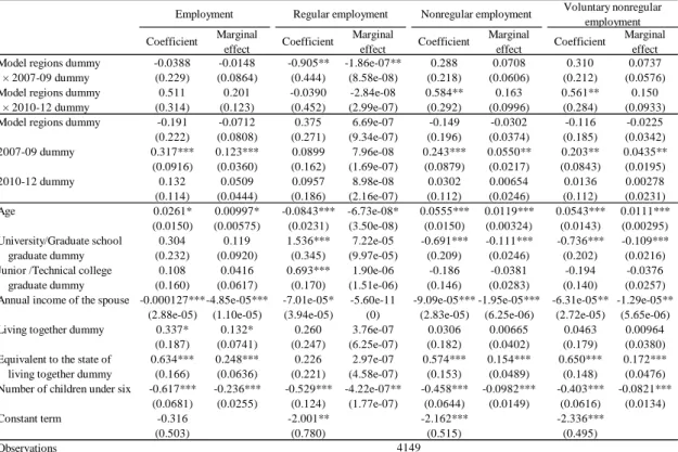
The results of DD analysis based on the regression model are shown in Tables 2–5. In the tables, both the coefficient and the marginal effect are reported. In each table, the case (1) indicates the estimation result where the financial index and financial scale, either of which could affect the attitudes of municipalities vis-à-vis child-rearing support, are not included in the independent variables, and the case (2) where these factors are included.

Looking at Table 2 (1), we find that the cross-term of the model region dummy and the year dummy is significantly positive only for non-regular employment and voluntary non-regular employment of 2010–12. Accordingly, we can interpret that the employment probability for non-regular employment, especially voluntary non-regular employment, in the target model regions was increased by the model programs. However, looking at the marginal effect, it is shown that the change is positive but not statistically significant, implying that the magnitude of the effect on non-regular employment and voluntary non-regular employment were not so large. Additionally, we could find that the cross-term with the 2007–09 dummy for regular employment is significantly negative for both the coefficient and marginal effect. Thus, we could understand that that the policy may have caused a decrease in the regular employment rate although the marginal effect is extremely small.

On the other hand, according to Table 2 (2) in which we control for regional factors such as financial index and financial scale, the cross-term of the model region dummy and year dummy is not significantly positive for both the coefficient and marginal effect whereas the financial index is significantly positive.

(17)

That is, after controlling for the regional factors, the significant policy effects on non-regular employment and voluntary non-regular employment from the 2010–12 period shown in Table 2 (1) disappears.

From this result, we can interpret that the effects seen in this period of child-rearing support policy stem mainly from the child-rearing support measures implemented and enhanced by the municipalities under the “Act for Measures to Support the Development of the Next Generation,” rather than by the designation of these municipalities as “model regions.”

Employment across individual attributes

Next, to examine the possibility that the child-rearing support policy has effects on women who bear specific attributes, the estimation is performed by taking the cross-term—which multiplies the model region dummy, the year dummy, and the dummy variables for the academic background or for the number of children. The estimation results are shown in Tables 3 and 4.

Looking at Table 3 (1) examining the differences in policy effects by academic background, the cross-term with the junior/technical college graduate dummy for the 2010–12 period of non-regular employment is significantly positive. Furthermore, the cross-term with the junior/technical college graduate dummy from the 2010–12 period of voluntary non-regular employment is significant for the coefficient. Thus, we could point out that married women who are junior/technical college graduates and living in the model regions had a higher probability of being employed as non-regular workers, in line with their wishes, following the policy implementation.

We can also confirm these results in Table 3 (2), in which regional factors such as the financial index are controlled for, implying that the positive effects on

(18)

non-regular employment among junior/technical college graduate married women are caused not only by child-rearing support measures at the municipal level, but also by the government’s “model region” designation.

In Table 4 (1), we can find that the cross-term with the dummy for having more than two children is significantly positive for the employment, non-regular employment, and voluntary non-regular employment of the 2010–12 period. Considering the fact that the cross-term with the dummy for having one child is not significant, we can say that a woman with more children tend to experience the effects of child-rearing support policy. However, in Table 4 (2) where we control for regional factors, these significant policy effects are not seen, implying that the child-rearing support policy for married women with more children was effective due to the measures undertaken by the municipalities, rather than the government’s model region program.

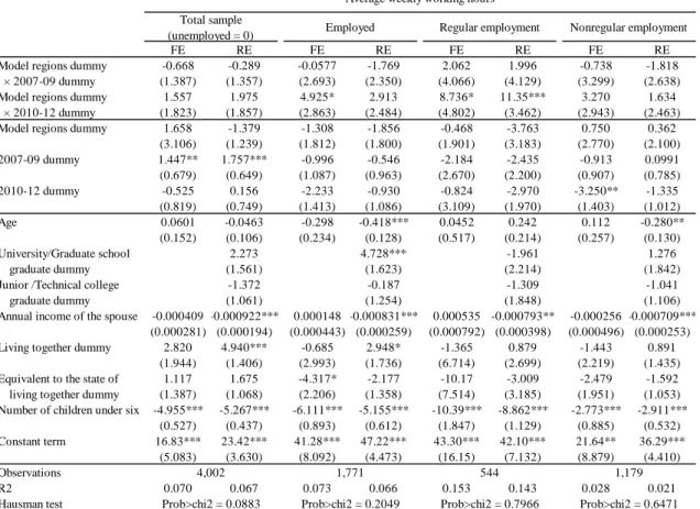
Hours of work

Table 5 shows the estimation results of the effects of child-rearing support policy on the average weekly working hours of women, by using fixed-effect and random-effect models. In these estimations, we put zero in the weekly working hours for the unemployed. As shown in the results of the Hausman test in the bottom row of Table 5, the fixed-effect model is adopted for the case using the whole sample, while the random-effect model is for other cases.

Looking at Table 5 (1), no significant coefficients are found for the cross-term of the model region dummy and year dummy for the case using the whole sample and the sample of being employed, in the model supported by the Hausman test. However, in the case using the sample of regular employment, positive and significant policy effects are obtained for the 2010–12 period in the random-effect

(19)

model, which is supported by the Hausman test. As shown in Table 5 (2), these results do not change, even if the regional factors are controlled for. In other words, we can interpret our findings as the “General Childcare-Support for Model-municipalities” reduced the burden of childcare for women employed as regular workers, and those women could increase their hours of work.

4.3 Results of DD analysis based on propensity score matching

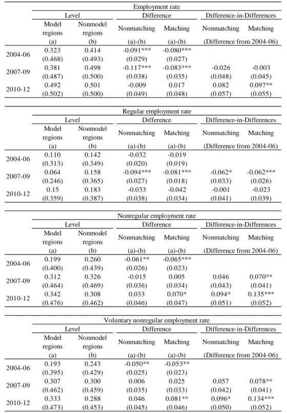
To confirm the robustness of the results of DD analysis based on the regression model, we show the results of propensity score matching in Table 6.

In Table 6, the employment rate, regular employment rate, non-regular employment rate, and voluntary non-regular employment rate are shown in rows (a) and (b) for the model regions and non-model regions within the period of 2004– 06, 2007–09, and 2010–12. The “Difference (a) – (b)” is the difference between each employment rate in model regions and non-model ones. Among these differences, “Nonmatching” is the simple difference, and “Matching” is the difference derived through the propensity score matching. In addition, “Difference-in-Differences” is the ATT from the nonmatching and matching methods, determined by the difference from the period 2004–06. If the child-rearing support policy is effective, this ATT should be significantly positive.

Without controlling for regional factors

In the same manner as the DD analysis based on the regression model, Table 6 shows the following cases: (1) without controlling for regional factors, and (2) with controlling for regional factors. Whether or not the regional factors are controlled refers to whether or not the financial index and financial scale are included in the explanatory variable 𝑿𝑿𝒊𝒊 of the probit model in equation (2) to

(20)

calculate the propensity score. Therefore, we can interpret that the ATT in Table 6 (1) incorporates the total effects of the child-rearing support policy introduced by the municipalities and of the government’s designation to the “model region,” and that the ATT in Table 6 (2) reflects the effects of the government’s designation.

Looking at the “Difference” in Table 6 (1), we can see that the difference for the employment rate is significantly negative for each of the 2004–06 and 2007– 09 periods, for both matching and nonmatching. This means that at the start of the policy implementation, the employment rate for women was significantly lower in the model regions than in the non-model regions. And, this result does not change, even when the attributes are controlled through propensity score matching.

In addition, we can see that the regular employment rate for 2007–09 and each of the non-regular employment rate and voluntary non-regular employment rate for 2004–06 are also significantly lower in the model regions, even when the attributes are controlled through propensity score matching. However, the negative significance of the non-regular employment rate and the voluntary non-regular employment rate is not observed during the model program period or in subsequent periods. Furthermore, the results of matching estimation for 2010–12 show that the rates in the model regions are significantly higher.

These tendencies are also shown in the “Difference-in-Differences” results. Specifically, for the non-regular employment rate and voluntary non-regular employment rate of 2007–09 and 2010–12, the ATT is significantly positive, both for matching and nonmatching. Furthermore, the ATT through propensity score matching for the employment rate is significantly positive for the 2010–12 period.

According to these results, the “General Childcare-Support for Model-municipalities” can be interpreted as having helped improve the non-regular

(21)

employment rate and voluntary non-regular employment rate—both of which were lower in the model regions than in the non-model regions—and increasing the probability of non-regular employment among women.

With controlling for regional factors

Next, we focus on the “Difference” in Table 6 (2), in which the regional factors are controlled for. First, the negative significance of the employment rate, regular employment rate, non-regular employment rate, and voluntary non-regular employment rate, which was shown in Table 6 (1), is not seen in Table 6 (2). Instead, we can occasionally find significantly positive differences. Therefore, we can infer that the lower employment rates in the model regions compared to the non-model regions—all of which are observed prior to the policy implementation— are caused by the regional factors such as financial index and financial scale, and that the employment environment prior to policy implementation was better in the model regions, according to a comparison of municipalities with similar regional factors.

Additionally, focusing on the “Difference-in-Differences” results, we find that the significantly positive ATTs for the employment rate and non-regular employment rate shown in Table 6 (1) are not estimated in Table 6 (2). Thus, we can determine that the effects of the child-rearing policy shown in Table 6 (1) were caused not by the government’s “model region” designation but mainly by the measures taken by the municipalities.

(22)

5. Concluding remarks

To promote the utilization of women in the labor market, developing an environment in which women can both work and take care of their children is highly important in Japan. However, no particular consensus has been obtained vis-à-vis the influence of child-rearing support policy undertaken by the government or the municipalities on the employment of women. In this paper, we estimate the effect of the local government’s child-rearing support policies implemented in Japan in the 2000s, the “General Childcare-Support for Model-municipalities.” We apply the standard method of the policy evaluation, regression and propensity score matching DD analysis, to derive the effect of the policy.

The main results we obtained can be summarized as follows. First, the “General Childcare-Support for Model-municipalities” increased the non-regular employment of women in the target model regions (municipalities)—especially voluntary non-regular employment. This tendency was more evident among women who are junior/technical college graduates and women with more children under the age of six. We also confirmed the tendency that the program increased the working hours of women who work as regular employees. On the other hand, we find that many of these policy effects disappear after controlling for the regional factors such as financial index and financial scale. This result implies that the effects of the program on women’s employment may depend more on the child-rearing support measures of the municipalities than on the government’s “model region” designation.

Considering these results, we could evaluate the “General Childcare-Support for Model-municipalities” as follows. First, focusing on the increase in non-regular employment—mainly in voluntary non-non-regular employment, we can say that

(23)

the “General Childcare-Support for Model-municipalities” has given rise to certain effects. If we observe the increase in non-regular employment through the involuntary non-regular employment, we should conclude that the child-rearing policy did not improve female labor market condition so that it increased the probability to find regular employment. However, our results indicate that the policy has supported women who want to work as non-regular workers, and thus the policy can be interpreted as having improved the employment environment for married women while parenting young children.

Next, the fact that the program has increased the working hours of married women who are employed as regular workers can be interpreted as follows. Generally speaking, in Japan, it is more difficult for women to be employed as regular workers than as non-regular workers. Thus, even if the childcare burden were reduced by the policy, it is not easy for married women to be employed as regular workers while parenting young children. In fact, we found that the child-rearing policy did not increase the regular employment rate among women. Instead of increasing the regular employment, the policy may have helped women who were working as regular workers prior to policy implementation reduce their childcare burden, thus allow them to spend more time working than would otherwise have been the case.

In line with the aforementioned results, we can conclude that the “General Childcare-Support for Model-municipalities” or the proactive child-rearing support measures by the municipalities under the “Act for Measures to Support the Development of the Next Generation” have had certain effects on women’s employment. However, we also find that many of these effects have been caused not by the government’s “model region” designation, but by measures taken at the municipal level. Therefore, we can point out that further investigation should be needed for the government’s model program in target regions.

(24)

Finally, we wish to address reservation and limitations in this study. Although we have examined the total effects of the “General Childcare-Support for Model-municipalities,” we did not examine in detail which programs are effective. As we described in Section 2, various child-rearing support programs included in the mandatory or optional programs have been implemented in the model regions. Due to the data limitation, however, we were not able to conduct detailed analysis to examine the effectiveness for various programs. This issue will be addressed in future research.

Next, this study addresses the short to middle-term effects of the “General Childcare-Support for Model-municipalities,” but it does not examine long-term effects. Although our results indicate policy effects vis-à-vis increases in the participation of women in non-regular employment and increases in the working hours of women who are employed as regular workers, it is possible that in the longer term, effects vis-à-vis increases in the probability of employment as a regular worker on account of reduced childcare burden could become more prominent. Particularly, as municipalities implemented long-term measures between 2005 and 2014 under the “Act for Measures to Support the Development of the Next Generation,” we can say that additional analysis that features an expanded target period is required.

(25)

References

Michael Baker, Jonathan Gruber and Kevin Milligan [2008] “Universal Child Care, Maternal Labor Supply, and Family Well-Being” Journal of Political

Economy, 2008, vol. 116, issue 4, pages 709-745.

Pierre Lefebvre and Philip Merrigan [2008] “Child-Care Policy and the Labor Supply of Mothers with Young Children: A Natural Experiment from Canada” Journal of Labor Economics, 2008, vol. 26, issue 3, pages 519-548. Pierre Lefebvre, Philip Merrigan and Matthieu Verstraete [2009] “Dynamic labor supply effects of childcare subsidies: Evidence from a Canadian natural experiment on low-fee universal child care” Labour Economics, 2009, vol. 16, issue 5, pages 490-502.

Akiko Ohishi [2003] “The influence of fee for day care on maternal employment”

Quarterly Journal of Social Security Research, vol.39, no.1, pages 55-69. (in

Japanese)

Akira Kawaguchi [2011] “The influence of long-term employment system and work– life balance measures on active participation by women” Report of the research on the relation between realization of work-life balance society and productivity, Economic and Social Research Institute, Cabinet Office, pages 81-96. (in Japanese)

Terukazu Suruga and Jianhua Zhang [2003] “Influence of parental leave programs on childbirths and continued employment of women: Quantitative analysis by panel data” Japanese Journal of Research on Household Economics, no.59, pages 56-63. (in Japanese)

Yasunobu Tomita [1994] “The effect of parental leave and work schedule on women’s retention after pregnancy” The Economic Review, vol.39, no.2, pages 43-56. (in Japanese)

(26)

Yoshio Higuchi [1994] “Empirical analysis of the parental leave,” Modern family

and social security, National Institute of Population and Social Security

Research ed., University of Tokyo Press, pages 181-204. (in Japanese) Yoshio Higuchi, Toshiyuki Matsuura and Kazuma Sato [2007] “Impact of Regional

Factors on Births and Wives’ Continuation in Employment: Panel survey of consumers by the Institute for Research on Household Economics”, RIETI Discussion Paper Series, 07-J-012. (in Japanese)

Hisakazu Matsushige and Mamiko Takeuchi [2008] “Effects of Intra-corporate Policies on the Work of Female Employees” Osaka School of International Public Policy Discussion Paper 13(1), pages 252-271. (in Japanese)

Katsura Maruyama [2001] “Practical Use of Working Women and the Analysis of Their Working Style after Childbirth” Journal of Population Problems, vol.57, no.2, pages 3-18. (in Japanese)

Yoko Morita and Yoshihiro Kaneko [1998] “The Effects of the Child Care Leave on Women in the Workforce” Journal of the Japan Institute of Labour, No.459, pages 50-60. (in Japanese)

Isamu Yamamoto [2011] “Involuntary Non-regular Workers in Japan and Their Mental Health”, Non-regular Employment System Reform in Japan:

Changing the way people work, Kotaro Tsuru, Yoshio Higuchi and Yuichiro

Mizumachi eds., Nippon Hyoron Sha Co., Ltd., Tokyo, Japan, Chapter 4, pages 93-120. (in Japanese)

Isamu Yamamoto [2014] “Workplace Environment and Female Employment: An empirical analysis using firm panel data” RIETI Discussion Paper Series, 14-J-017. (in Japanese)

(27)

Table 1 Basic statistics

Note: The numbers in parentheses are standard deviations.

Variable Model regions Nonmodel regions

0.38 0.46 (0.48) (0.50) 0.11 0.16 (0.31) (0.36) 0.26 0.29 (0.44) (0.45) 0.25 0.27 (0.44) (0.44) 10.99 14.15 (16.17) (18.11) 33.78 33.75 (3.97) (3.94) 0.19 0.13 (0.40) (0.34) 0.29 0.26 (0.45) (0.44) 4824.52 4675.04 (1904.40) (1941.71) 0.05 0.11 (0.22) (0.31) 0.10 0.11 (0.31) (0.31) 0.97 0.84 (0.82) (0.84) 0.40 0.37 (0.49) (0.48) 0.27 0.22 (0.45) (0.41) 0.88 0.80 (0.22) (0.23) 75700.00 44000.00 (34900.00) (38300.00) Obervations 682 3858

Voluntary nonregular employment dummy

Women Employment dummy

Regular employment dummy Nonregular employment dummy

Standard financial scale (unit: 1,000 yen) Average weekly working hours Age

University/Graduate school graduate dummy Junior/Technical college graduate dummy Annual income of the spouse (unit: 1,000 yen) Living together dummy

Equivalent to the state of living together dummy Number of children under six

With one child dummy

With more than two children dummy Financial index

(28)

Table 2 Estimation results for employment (1) Without controlling for regional factors

Note: 1) The numbers in parentheses are robust standard errors.

2) *, **, and *** indicate statistical significance at the 10, 5, and 1% levels, respectively.

Coefficient Marginal effect Coefficient Marginal effect Coefficient Marginal effect Coefficient Marginal effect -0.0388 -0.0148 -0.905** -1.86e-07** 0.288 0.0708 0.310 0.0737 (0.229) (0.0864) (0.444) (8.58e-08) (0.218) (0.0606) (0.212) (0.0576) 0.511 0.201 -0.0390 -2.84e-08 0.584** 0.163 0.561** 0.150 (0.314) (0.123) (0.452) (2.99e-07) (0.292) (0.0996) (0.284) (0.0933) -0.191 -0.0712 0.375 6.69e-07 -0.149 -0.0302 -0.116 -0.0225 (0.222) (0.0808) (0.271) (9.34e-07) (0.196) (0.0374) (0.185) (0.0342) 0.317*** 0.123*** 0.0899 7.96e-08 0.243*** 0.0550** 0.203** 0.0435** (0.0916) (0.0360) (0.162) (1.69e-07) (0.0879) (0.0217) (0.0843) (0.0195) 0.132 0.0509 0.0957 8.98e-08 0.0302 0.00654 0.0136 0.00278 (0.114) (0.0444) (0.186) (2.16e-07) (0.112) (0.0246) (0.112) (0.0231) 0.0261* 0.00997* -0.0843*** -6.73e-08* 0.0555*** 0.0119*** 0.0543*** 0.0111*** (0.0150) (0.00575) (0.0231) (3.50e-08) (0.0150) (0.00324) (0.0143) (0.00295) 0.304 0.119 1.536*** 7.22e-05 -0.691*** -0.111*** -0.736*** -0.109*** (0.232) (0.0920) (0.345) (9.97e-05) (0.209) (0.0246) (0.202) (0.0216) 0.108 0.0416 0.693*** 1.90e-06 -0.186 -0.0381 -0.194 -0.0376 (0.160) (0.0617) (0.170) (1.51e-06) (0.146) (0.0283) (0.140) (0.0257) -0.000127***-4.85e-05*** -7.01e-05* -5.60e-11 -9.09e-05*** -1.95e-05*** -6.31e-05** -1.29e-05**

(2.88e-05) (1.10e-05) (3.94e-05) (0) (2.83e-05) (6.25e-06) (2.72e-05) (5.65e-06) 0.337* 0.132* 0.260 3.76e-07 0.0306 0.00665 0.0463 0.00964 (0.187) (0.0741) (0.247) (6.25e-07) (0.182) (0.0402) (0.179) (0.0380) 0.634*** 0.248*** 0.226 2.97e-07 0.574*** 0.154*** 0.650*** 0.172*** (0.166) (0.0636) (0.221) (4.58e-07) (0.153) (0.0489) (0.148) (0.0476) -0.617*** -0.236*** -0.529*** -4.22e-07** -0.458*** -0.0982*** -0.403*** -0.0821*** (0.0681) (0.0255) (0.124) (1.77e-07) (0.0644) (0.0149) (0.0616) (0.0134) -0.316 -2.001** -2.162*** -2.336*** (0.503) (0.780) (0.515) (0.495) Observations

Annual income of the spouse

Employment Regular employment Nonregular employment Voluntary nonregular employment

Model regions dummy × 2010-12 dummy Model regions dummy

2010-12 dummy

Age

University/Graduate school graduate dummy Junior /Technical college graduate dummy Model regions dummy × 2007-09 dummy

2007-09 dummy

Living together dummy

Constant term

(29)

(2) With controlling for regional factors

Coefficient Marginal effect Coefficient Marginal effect Coefficient Marginal effect Coefficient Marginal effect 0.223 0.0870 -0.784 -1.47e-07 0.434 0.121 0.456 0.123 (0.294) (0.117) (0.594) (1.56e-06) (0.293) (0.0943) (0.281) (0.0888) 0.498 0.196 1.088* 1.95e-05 0.266 0.0697 0.279 0.0702 (0.449) (0.176) (0.602) (0.000169) (0.434) (0.127) (0.419) (0.119) 0.205 0.0797 -0.0523 -3.07e-08 0.191 0.0473 0.195 0.0461 (0.293) (0.115) (0.343) (3.37e-07) (0.277) (0.0729) (0.260) (0.0656) 0.187 0.0720 -0.0202 -1.28e-08 0.121 0.0286 0.0806 0.0181 (0.129) (0.0503) (0.242) (2.30e-07) (0.125) (0.0305) (0.120) (0.0275) 0.203 0.0785 -0.188 -9.33e-08 0.208 0.0515 0.143 0.0331 (0.195) (0.0766) (0.327) (1.01e-06) (0.176) (0.0469) (0.174) (0.0424) 0.0190 0.00725 -0.0716** -4.61e-08 0.0473** 0.0110** 0.0497*** 0.0110*** (0.0202) (0.00771) (0.0314) (4.74e-07) (0.0187) (0.00437) (0.0181) (0.00405) 0.101 0.0389 1.183*** 1.86e-05 -0.619** -0.110*** -0.589** -0.100*** (0.308) (0.120) (0.385) (0.000156) (0.278) (0.0367) (0.264) (0.0336) 0.0801 0.0307 1.053*** 5.28e-06 -0.346* -0.0740** -0.363** -0.0733** (0.198) (0.0762) (0.265) (4.75e-05) (0.184) (0.0359) (0.178) (0.0326) -9.98e-05** -3.80e-05** -0.000119** -7.69e-11 -6.47e-05 -1.50e-05 -3.95e-05 -8.71e-06 (4.37e-05) (1.66e-05) (5.90e-05) (8.01e-10) (4.04e-05) (9.43e-06) (3.86e-05) (8.55e-06)

0.315 0.123 -0.0990 -5.22e-08 0.165 0.0410 0.182 0.0433 (0.205) (0.0812) (0.359) (5.12e-07) (0.195) (0.0516) (0.200) (0.0514) 0.766*** 0.298*** 0.329 4.53e-07 0.638*** 0.185*** 0.721*** 0.206*** (0.212) (0.0786) (0.255) (4.68e-06) (0.187) (0.0640) (0.182) (0.0621) -0.667*** -0.254*** -0.445*** -2.87e-07 -0.537*** -0.124*** -0.464*** -0.102*** (0.0983) (0.0368) (0.171) (2.99e-06) (0.0897) (0.0213) (0.0846) (0.0191) -0.250 -0.0951 -2.006*** -1.29e-06 0.634* 0.147* 0.592* 0.131* (0.372) (0.142) (0.535) (1.34e-05) (0.331) (0.0774) (0.311) (0.0691) -0.165 -0.0629 -0.227 -1.46e-07 -0.0983 -0.0228 -0.110 -0.0242 (0.107) (0.0409) (0.153) (1.50e-06) (0.101) (0.0234) (0.0967) (0.0214) 2.878 3.359 -0.718 -0.782 (1.919) (2.540) (1.764) (1.696) Observations Model regions dummy × 2007-09 dummy

Model regions dummy

2010-12 dummy 2007-09 dummy

Number of children under six

Financial index

University/Graduate school graduate dummy Junior /Technical college graduate dummy Annual income of the spouse

Living together dummy

Equivalent to the state of living together dummy Age

Employment Regular employment Nonregular employment Voluntary nonregular employment

Model regions dummy × 2010-12 dummy

2279 ln standard financial scale

(30)

Table3 Estimation results for employment across the academic background (1) Without controlling for regional factors

Coefficient Marginal effect Coefficient Marginal effect Coefficient Marginal effect Coefficient Marginal effect -0.409 -0.143 0.120 0.0273 -0.0375 -0.00747 (0.741) (0.232) (0.671) (0.163) (0.562) (0.110) -0.332 -0.119 -3.129*** -1.05e-07** 0.122 0.0280 0.138 0.0304 (0.439) (0.145) (0.586) (4.91e-08) (0.463) (0.113) (0.454) (0.107) -0.149 -0.0555 -2.006 -8.85e-08** 0.295 0.0736 0.332 0.0808 (0.831) (0.301) (1.955) (4.15e-08) (0.845) (0.240) (0.813) (0.230) 0.816 0.315 -1.981*** -9.13e-08** 1.119** 0.368* 0.971* 0.301 (0.608) (0.213) (0.711) (4.31e-08) (0.547) (0.217) (0.524) (0.205) 0.118 0.0457 0.0309 1.50e-08 0.237 0.0569 0.274 0.0640 (0.280) (0.110) (0.402) (2.09e-07) (0.256) (0.0681) (0.251) (0.0661) 0.289 0.114 0.701 2.58e-06 0.169 0.0396 0.186 0.0419 (0.461) (0.184) (0.628) (7.74e-06) (0.410) (0.104) (0.397) (0.0978) -0.192 -0.0717 0.226 1.64e-07 -0.162 -0.0325 -0.124 -0.0240 (0.227) (0.0824) (0.250) (2.75e-07) (0.198) (0.0373) (0.187) (0.0344) 0.318*** 0.123*** 0.0769 3.79e-08 0.244*** 0.0552** 0.204** 0.0436** (0.0917) (0.0360) (0.163) (9.32e-08) (0.0879) (0.0217) (0.0844) (0.0195) 0.132 0.0509 0.0777 3.99e-08 0.0318 0.00690 0.0151 0.00309 (0.114) (0.0444) (0.188) (1.15e-07) (0.112) (0.0246) (0.112) (0.0231) 0.0260* 0.00994* -0.0838*** -3.77e-08* 0.0549*** 0.0118*** 0.0538*** 0.0110*** (0.0151) (0.00576) (0.0238) (2.07e-08) (0.0150) (0.00324) (0.0144) (0.00295) 0.328 0.128 1.640*** 6.96e-05 -0.699*** -0.111*** -0.740*** -0.109*** (0.236) (0.0934) (0.360) (0.000101) (0.213) (0.0249) (0.205) (0.0219) 0.101 0.0387 0.779*** 1.51e-06 -0.220 -0.0445 -0.225 -0.0431* (0.161) (0.0624) (0.173) (1.23e-06) (0.148) (0.0283) (0.143) (0.0257) -0.000126*** -4.81e-05*** -6.59e-05* -0 -9.04e-05*** -1.94e-05*** -6.25e-05** -1.27e-05**

(2.87e-05) (1.10e-05) (4.00e-05) (0) (2.82e-05) (6.21e-06) (2.71e-05) (5.62e-06)

0.334* 0.131* 0.269 2.27e-07 0.0224 0.00486 0.0392 0.00812 (0.188) (0.0745) (0.247) (3.75e-07) (0.183) (0.0400) (0.179) (0.0378) 0.638*** 0.250*** 0.182 1.23e-07 0.584*** 0.157*** 0.659*** 0.175*** (0.166) (0.0636) (0.221) (2.18e-07) (0.153) (0.0490) (0.148) (0.0477) -0.618*** -0.236*** -0.556*** -2.50e-07** -0.456*** -0.0978*** -0.401*** -0.0817*** (0.0681) (0.0255) (0.129) (1.09e-07) (0.0644) (0.0148) (0.0615) (0.0133) -0.320 -2.112*** -2.137*** -2.315*** (0.504) (0.796) (0.517) (0.496) Observations

Model regions dummy × 2007-09 dummy × University/Graduate school graduate dummy Model regions dummy × 2007-09 dummy × Junior/Technical college graduate dummy

Model regions dummy × 2007-09 dummy Voluntary nonregular employment Nonregular employment Regular employment Employment 2007-09 dummy

Model regions dummy × 2010-12 dummy × University/Graduate school graduate dummy Model regions dummy × 2010-12 dummy × Junior/Technical college graduate dummy

2010-12 dummy Age University/Graduate school graduate dummy Junior/Technical college graduate dummy Annual income of the spouse Living together dummy Equivalent to the state of living together dummy Number of children under six Constant term

4149 4149

4116 4149

(31)

Coefficient Marginal effect Coefficient Marginal effect Coefficient Marginal effect Coefficient Marginal effect 0.0851 0.0328 0.222 0.0563 -0.0664 -0.0138 (1.019) (0.397) (0.971) (0.272) (0.775) (0.156) -0.0941 -0.0353 -2.104*** -1.80e-07 0.295 0.0771 0.277 0.0689 (0.465) (0.171) (0.813) (1.77e-06) (0.482) (0.142) (0.472) (0.132) 0.653 0.256 1.450 0.506 1.373 0.470 (1.182) (0.445) (1.129) (0.419) (1.062) (0.410) 1.781** 0.555*** -2.657*** -1.69e-07 2.486*** 0.781*** 2.152*** 0.717*** (0.771) (0.111) (0.806) (1.67e-06) (0.703) (0.107) (0.675) (0.159) 0.234 0.0913 -0.0401 -2.83e-08 0.299 0.0776 0.368 0.0942 (0.355) (0.141) (0.702) (4.86e-07) (0.336) (0.0977) (0.327) (0.0962) -0.175 -0.0647 2.286*** 0.00183 -0.795* -0.116*** -0.681 -0.100** (0.553) (0.197) (0.689) (0.0107) (0.442) (0.0377) (0.427) (0.0394) 0.204 0.0789 -0.0505 -3.57e-08 0.194 0.0471 0.203 0.0473 (0.295) (0.116) (0.335) (3.64e-07) (0.282) (0.0730) (0.265) (0.0662) 0.191 0.0734 -0.0233 -1.77e-08 0.127 0.0295 0.0864 0.0190 (0.130) (0.0506) (0.239) (2.77e-07) (0.126) (0.0303) (0.121) (0.0273) 0.205 0.0791 -0.195 -1.15e-07 0.216 0.0526 0.151 0.0343 (0.197) (0.0772) (0.327) (1.14e-06) (0.179) (0.0469) (0.176) (0.0424) 0.0183 0.00697 -0.0702** -5.43e-08 0.0461** 0.0105** 0.0486*** 0.0105*** (0.0205) (0.00779) (0.0313) (5.11e-07) (0.0191) (0.00435) (0.0184) (0.00403) 0.0869 0.0333 1.328*** 3.96e-05 -0.675** -0.114*** -0.631** -0.103*** (0.316) (0.122) (0.387) (0.000299) (0.287) (0.0353) (0.272) (0.0328) 0.0324 0.0124 1.181*** 9.32e-06 -0.447** -0.0911*** -0.453** -0.0875*** (0.205) (0.0784) (0.267) (7.56e-05) (0.195) (0.0353) (0.188) (0.0323) -9.93e-05** -3.78e-05** -0.000113* -8.72e-11 -6.75e-05* -1.53e-05 -4.16e-05 -9.00e-06 (4.38e-05) (1.67e-05) (5.88e-05) (8.36e-10) (4.08e-05) (9.33e-06) (3.90e-05) (8.47e-06)

0.312 0.122 -0.0687 -4.62e-08 0.154 0.0372 0.172 0.0402 (0.206) (0.0816) (0.359) (4.23e-07) (0.195) (0.0502) (0.201) (0.0503) 0.793*** 0.308*** 0.276 3.98e-07 0.689*** 0.199*** 0.770*** 0.220*** (0.213) (0.0784) (0.264) (3.81e-06) (0.187) (0.0646) (0.182) (0.0626) -0.672*** -0.256*** -0.450** -3.48e-07 -0.545*** -0.124*** -0.469*** -0.101*** (0.0997) (0.0373) (0.176) (3.32e-06) (0.0906) (0.0214) (0.0850) (0.0191) -0.294 -0.112 -2.053*** -1.59e-06 0.616* 0.140* 0.581* 0.126* (0.373) (0.142) (0.538) (1.51e-05) (0.338) (0.0775) (0.316) (0.0692) -0.165 -0.0628 -0.228 -1.76e-07 -0.0977 -0.0222 -0.109 -0.0235 (0.109) (0.0414) (0.153) (1.66e-06) (0.102) (0.0233) (0.0984) (0.0214) 2.943 3.325 -0.648 -0.732 (1.941) (2.580) (1.795) (1.727) Observations Constant term

Annual income of the spouse

Living together dummy 2010-12 dummy

Age

University/Graduate school graduate dummy

Model regions dummy × 2010-12 dummy × University/Graduate school graduate dummy Model regions dummy × 2010-12 dummy × Junior/Technical college graduate dummy Model regions dummy

× 2007-09 dummy

Junior/Technical college graduate dummy

2279

Nonregular employment Voluntary nonregular employment

2279 Model regions dummy × 2007-09 dummy

× University/Graduate school graduate dummy Model regions dummy × 2007-09 dummy × Junior/Technical college graduate dummy

Employment Regular employment

2007-09 dummy

2252 2279

Financial index

(32)

Table4 Estimation results for employment across the number of children

(1) Without controlling for regional factors

Coefficient Marginal effect Coefficient Marginal effect Coefficient Marginal effect Coefficient Marginal effect 0.467 0.184 0.333 6.99e-07 0.118 0.0269 0.0184 0.00378 (0.395) (0.155) (0.879) (3.67e-06) (0.356) (0.0861) (0.345) (0.0717) -0.232 -0.0851 -0.453 -1.51e-07 0.0426 0.00935 -0.0297 -0.00594 (0.458) (0.160) (0.876) (1.06e-07) (0.480) (0.108) (0.475) (0.0935) 0.164 0.0640 0.474 1.57e-06 0.149 0.0345 -0.0459 -0.00910 (0.483) (0.191) (0.816) (6.73e-06) (0.456) (0.114) (0.442) (0.0853) 1.179** 0.428*** -0.381 -1.42e-07 1.213** 0.405* 1.074** 0.342 (0.541) (0.147) (0.791) (1.17e-07) (0.557) (0.220) (0.548) (0.217) -0.201 -0.0744 -0.936 -1.99e-07** 0.199 0.0469 0.285 0.0667 (0.348) (0.124) (0.748) (9.43e-08) (0.304) (0.0783) (0.300) (0.0797) 0.179 0.0700 -0.0941 -6.40e-08 0.217 0.0518 0.299 0.0709 (0.350) (0.138) (0.508) (2.74e-07) (0.338) (0.0892) (0.331) (0.0900) -0.179 -0.0668 0.351 6.25e-07 -0.117 -0.0239 -0.0876 -0.0172 (0.218) (0.0797) (0.274) (9.03e-07) (0.193) (0.0378) (0.183) (0.0347) 0.319*** 0.123*** 0.114 1.11e-07 0.241*** 0.0545** 0.201** 0.0429** (0.0915) (0.0360) (0.158) (1.90e-07) (0.0883) (0.0218) (0.0848) (0.0195) 0.128 0.0496 0.107 1.09e-07 0.0237 0.00512 0.00999 0.00204 (0.114) (0.0444) (0.188) (2.40e-07) (0.112) (0.0244) (0.112) (0.0230) 0.0233 0.00893 -0.0854*** -7.23e-08* 0.0533*** 0.0114*** 0.0524*** 0.0107*** (0.0150) (0.00575) (0.0233) (3.76e-08) (0.0150) (0.00323) (0.0144) (0.00294) 0.345 0.135 1.568*** 8.46e-05 -0.661*** -0.107*** -0.710*** -0.106*** (0.231) (0.0916) (0.358) (0.000120) (0.208) (0.0250) (0.201) (0.0219) 0.125 0.0480 0.707*** 2.11e-06 -0.174 -0.0357 -0.185 -0.0357 (0.159) (0.0615) (0.173) (1.69e-06) (0.145) (0.0284) (0.140) (0.0257) -0.000134*** -5.12e-05*** -7.18e-05* -6.08e-11 -9.56e-05*** -2.05e-05*** -6.70e-05** -1.36e-05**

(2.89e-05) (1.11e-05) (4.04e-05) (0) (2.84e-05) (6.27e-06) (2.73e-05) (5.66e-06)

0.388** 0.152** 0.273 4.32e-07 0.0620 0.0137 0.0725 0.0153 (0.187) (0.0739) (0.252) (7.12e-07) (0.183) (0.0413) (0.179) (0.0389) 0.651*** 0.255*** 0.266 4.10e-07 0.582*** 0.156*** 0.656*** 0.174*** (0.163) (0.0620) (0.216) (5.68e-07) (0.152) (0.0489) (0.148) (0.0476) -0.912*** -0.325*** -0.896*** -8.85e-07** -0.613*** -0.121*** -0.518*** -0.0980*** (0.118) (0.0378) (0.185) (4.33e-07) (0.109) (0.0213) (0.105) (0.0196) -1.319*** -0.409*** -1.032*** -5.47e-07** -1.014*** -0.160*** -0.897*** -0.138*** (0.148) (0.0342) (0.245) (2.46e-07) (0.140) (0.0203) (0.136) (0.0188) -0.0968 -1.851** -2.015*** -2.216*** (0.503) (0.782) (0.517) (0.498) (0.0189) Observations 4149

Equivalent to the state of living together dummy With one child dummy

With more than two children dummy Constant term

Junior/Technical college graduate dummy Annual income of the spouse Living together dummy 2010-12 dummy Age

University/Graduate school graduate dummy Model regions dummy × 2010-12 dummy Model regions dummy 2007-09 dummy

Model regions dummy × 2010-12 dummy × With one child dummy

Model regions dummy × 2010-12 dummy × With more than two children dummy Model regions dummy

× 2007-09 dummy

Nonregular employment Voluntary nonregular employment

Model regions dummy × 2007-09 dummy × With more than two children dummy

(33)

Coefficient Marginal effect Coefficient Marginal effect Coefficient Marginal effect Coefficient Marginal effect -0.372 -0.132 -2.225 -4.37e-08 -0.0944 -0.0208 -0.248 -0.0478 (0.481) (0.155) (1.653) (7.59e-07) (0.444) (0.0931) (0.431) (0.0715) -1.353*** -0.338*** -2.510* -4.04e-08 -0.549 -0.0936 -0.654 -0.0985* (0.522) (0.0625) (1.475) (7.05e-07) (0.551) (0.0646) (0.546) (0.0510) -0.0559 -0.0211 0.539 5.28e-07 0.0705 0.0169 -0.229 -0.0445 (0.612) (0.229) (0.896) (8.76e-06) (0.585) (0.145) (0.567) (0.0956) 0.980 0.370 -1.268 -3.43e-08 1.069 0.361 0.854 0.268 (0.734) (0.233) (1.471) (6.05e-07) (0.775) (0.308) (0.763) (0.295) 0.752* 0.293* 0.488 3.66e-07 0.600 0.176 0.718* 0.211 (0.446) (0.163) (0.675) (5.54e-06) (0.414) (0.145) (0.404) (0.146) 0.354 0.139 1.229 1.26e-05 0.0632 0.0151 0.219 0.0537 (0.553) (0.220) (0.896) (0.000156) (0.541) (0.133) (0.523) (0.141) 0.246 0.0957 -0.173 -2.39e-08 0.229 0.0572 0.227 0.0543 (0.295) (0.116) (0.445) (3.90e-07) (0.276) (0.0742) (0.259) (0.0668) 0.184 0.0709 -0.00902 -1.65e-09 0.115 0.0272 0.0757 0.0169 (0.129) (0.0500) (0.270) (6.81e-08) (0.125) (0.0305) (0.120) (0.0275) 0.191 0.0741 -0.179 -2.55e-08 0.197 0.0485 0.137 0.0315 (0.194) (0.0759) (0.353) (4.55e-07) (0.176) (0.0463) (0.173) (0.0420) 0.0158 0.00604 -0.0707* -1.30e-08 0.0442** 0.0102** 0.0472*** 0.0104*** (0.0201) (0.00767) (0.0373) (2.18e-07) (0.0185) (0.00430) (0.0180) (0.00401) 0.137 0.0528 1.182*** 6.45e-06 -0.583** -0.105*** -0.557** -0.0960*** (0.305) (0.120) (0.435) (8.81e-05) (0.278) (0.0377) (0.264) (0.0345) 0.106 0.0408 1.073*** 1.85e-06 -0.321* -0.0688* -0.345* -0.0697** (0.198) (0.0763) (0.321) (2.70e-05) (0.184) (0.0363) (0.178) (0.0329) -0.000103** -3.94e-05** -0.000122** -0 -6.82e-05* -1.58e-05* -4.18e-05 -9.20e-06 (4.34e-05) (1.65e-05) (6.15e-05) (3.82e-10) (4.03e-05) (9.40e-06) (3.86e-05) (8.53e-06)

0.350* 0.137* -0.115 -1.67e-08 0.205 0.0515 0.216 0.0522 (0.203) (0.0804) (0.372) (2.73e-07) (0.195) (0.0531) (0.201) (0.0530) 0.791*** 0.308*** 0.319 1.27e-07 0.643*** 0.186*** 0.731*** 0.209*** (0.206) (0.0759) (0.255) (2.17e-06) (0.185) (0.0636) (0.181) (0.0621) -0.935*** -0.333*** -0.425 -7.33e-08 -0.822*** -0.173*** -0.682*** -0.138*** (0.165) (0.0531) (0.266) (1.25e-06) (0.144) (0.0295) (0.140) (0.0276) -1.392*** -0.425*** -0.872** -1.02e-07 -1.141*** -0.192*** -0.980*** -0.162*** (0.214) (0.0478) (0.374) (1.72e-06) (0.188) (0.0273) (0.177) (0.0253) -0.291 -0.111 -2.019*** -3.72e-07 0.623* 0.144* 0.576* 0.127* (0.365) (0.139) (0.614) (6.30e-06) (0.329) (0.0768) (0.309) (0.0686) -0.171 -0.0652 -0.227 -4.19e-08 -0.106 -0.0245 -0.114 -0.0250 (0.106) (0.0406) (0.167) (7.02e-07) (0.100) (0.0233) (0.0967) (0.0214) 3.219* 3.128 -0.364 -0.539 (1.894) (2.578) (1.750) (1.691) (0.0189) Observations 2279 Financial index Constant term Equivalent to the state of living together dummy With one child dummy

With more than two children dummy

ln standard financial scale Annual income of the spouse Living together dummy Junior/Technical college graduate dummy

Voluntary nonregular employment

Model regions dummy × 2007-09 dummy × With more than two children dummy

2010-12 dummy Age

University/Graduate school graduate dummy 2007-09 dummy

Model regions dummy × 2010-12 dummy × With more than two children dummy Model regions dummy

× 2007-09 dummy

(34)

Table 5 Estimation results for working hours (1) Without controlling for regional factors

2) *, **, and *** indicate statistical significance at the 10, 5, and 1% levels, respectively. 3) FE indicates fixed-effect model, and RE indicates random-effect model.

FE RE FE RE FE RE FE RE -0.668 -0.289 -0.0577 -1.769 2.062 1.996 -0.738 -1.818 (1.387) (1.357) (2.693) (2.350) (4.066) (4.129) (3.299) (2.638) 1.557 1.975 4.925* 2.913 8.736* 11.35*** 3.270 1.634 (1.823) (1.857) (2.863) (2.484) (4.802) (3.462) (2.943) (2.463) 1.658 -1.379 -1.308 -1.856 -0.468 -3.763 0.750 0.362 (3.106) (1.239) (1.812) (1.800) (1.901) (3.183) (2.770) (2.100) 1.447** 1.757*** -0.996 -0.546 -2.184 -2.435 -0.913 0.0991 (0.679) (0.649) (1.087) (0.963) (2.670) (2.200) (0.907) (0.785) -0.525 0.156 -2.233 -0.930 -0.824 -2.970 -3.250** -1.335 (0.819) (0.749) (1.413) (1.086) (3.109) (1.970) (1.403) (1.012) 0.0601 -0.0463 -0.298 -0.418*** 0.0452 0.242 0.112 -0.280** (0.152) (0.106) (0.234) (0.128) (0.517) (0.214) (0.257) (0.130) 2.273 4.728*** -1.961 1.276 (1.561) (1.623) (2.214) (1.842) -1.372 -0.187 -1.309 -1.041 (1.061) (1.254) (1.848) (1.106) -0.000409 -0.000922*** 0.000148 -0.000831*** 0.000535 -0.000793** -0.000256 -0.000709*** (0.000281) (0.000194) (0.000443) (0.000259) (0.000792) (0.000398) (0.000496) (0.000253) 2.820 4.940*** -0.685 2.948* -1.365 0.879 -1.443 0.891 (1.944) (1.406) (2.993) (1.736) (6.714) (2.699) (2.219) (1.435) 1.117 1.675 -4.317* -2.177 -10.17 -3.009 -2.479 -1.592 (1.387) (1.068) (2.206) (1.358) (7.514) (3.185) (1.951) (1.053) -4.955*** -5.267*** -6.111*** -5.155*** -10.39*** -8.862*** -2.773*** -2.911*** (0.527) (0.437) (0.893) (0.612) (1.847) (1.129) (0.885) (0.532) 16.83*** 23.42*** 41.28*** 47.22*** 43.30*** 42.10*** 21.64** 36.29*** (5.083) (3.630) (8.092) (4.473) (16.15) (7.132) (8.879) (4.410) Observations R2 0.070 0.067 0.073 0.066 0.153 0.143 0.028 0.021 Hausman test 1,179 544 1,771 4,002

Junior /Technical college graduate dummy

Number of children under six Constant term

Average weekly working hours Total sample

(unemployed = 0) Employed Regular employment Nonregular employment Model regions dummy

× 2007-09 dummy

2007-09 dummy

Annual income of the spouse Living together dummy Equivalent to the state of living together dummy Model regions dummy × 2010-12 dummy Model regions dummy

2010-12 dummy Age

University/Graduate school graduate dummy

Prob>chi2 = 0.2049 Prob>chi2 = 0.7966 Prob>chi2 = 0.6471 Prob>chi2 = 0.0883