Eigenvalue problems associated with 1-dimensional scalar field equations (Succession and Innovation of Studies on ODEs in Real Domains)

全文

(1)94. 数理解析研究所講究録第2080巻 2018年 94-105. Eigenvalue problems associated with 1‐dimensional scalar field equations Tohru Wakasa. Kyushu Institute of Technology. 1. Introduction. Let us consider the boundary value problem. Here. \left{\begin{ar y}{l $\varepsilon$^{2}u_{x}+f(u)=0,\mathrm{i}\mathrm{n}(0,1)\ u_{x}(0)=u_{x}(1)=0,\ u>0,\mathrm{i}\mathrm{n}(0,1). \end{ar y}\right.. $\varepsilon$. (NP). is a positive parameter and. f(u)=-u+u^{p} with. p> 1 .. The problem (NP) is called the scalar field equation, which is motivated by. the parabolic PDEs modelling pattern formation and chemotaxis, and also by PDEs of. Klein‐Gordon/nonlinear Schrödinger type ([2] and [4]). In the 1‐D problem (NP) a classical shooting argument solves the global bifurcation structure of all solutions ([5]). In particular, one can observe the families of periodic solutions: for any n , there exist $\varepsilon$_{n} > 0 such that there exist 1/n‐periodic solutions u_{n, $\varepsilon$}^{\pm}(x) for $\varepsilon$\in(0, $\varepsilon$_{n}) ;. u_{n, $\varepsilon$}^{+}(0)=\displaystyle \max_{x\in[0,1]}u_{n, $\varepsilon$}^{+}(x) , u_{n, $\varepsilon$}^{-}(0)=\min_{x\in[0,1]}u_{n, $\varepsilon$}^{-}(x) . In view of pattern formation, we say. (1.1). u_{n, $\varepsilon$}^{+} is interior spike solution, and u_{\overline{n},$\varepsilon$} is boundary. spike solution. We fix n\in \mathrm{N} arbitrarily and assume problems associated with u_{n, $\varepsilon$}^{+} and u_{\overline{n}, $\varepsilon$}. $\varepsilon$\in. (0, $\varepsilon$_{n}) . Consider the linearized eigenvalue. \left\{ begin{ar y}{l $\varepsilon$^{2}$\varphi$_{x }(x)+f_{u}( _{n,$\varepsilon$}^{\pm}(x) $\varphi$(x)+$\lambda\varphi$(x)=0&\mathrm{i}\mathrm{n}(0,1),\ $\varphi$_{x}(0)=$\varphi$_{x}(1)=0.& \end{ar y}\right.. (\mathrm{L}\mathrm{P}_{\pm}). For j\in \mathrm{N}\cup\{0\} we denote by $\lambda$_{j}^{\pm}=$\lambda$_{j, $\varepsilon$}^{\pm} and $\varphi$_{j}^{\pm}(x)=$\varphi$_{j, $\varepsilon$}^{\pm}(x) , the (j+1) ‐th eigenvalue and the corresponding eigenfunction, respectively. By the Sturm‐Liouville theory shows that. $\lambda$_{0, $\varepsilon$}^{+}<$\lambda$_{1, $\varepsilon$}^{+}<\cdots<$\lambda$_{j, $\varepsilon$}^{+}<\cdots<+\infty, $\lambda$_{0, $\varepsilon$}^{-}<$\lambda$_{1, $\varepsilon$}^{-}<\cdots<$\lambda$_{j, $\varepsilon$}^{-}<\cdots<+\infty, and the both. $\varphi$_{j,$\varepsilon$}^{\pm}. have exactly j zeros in (0,1) ..

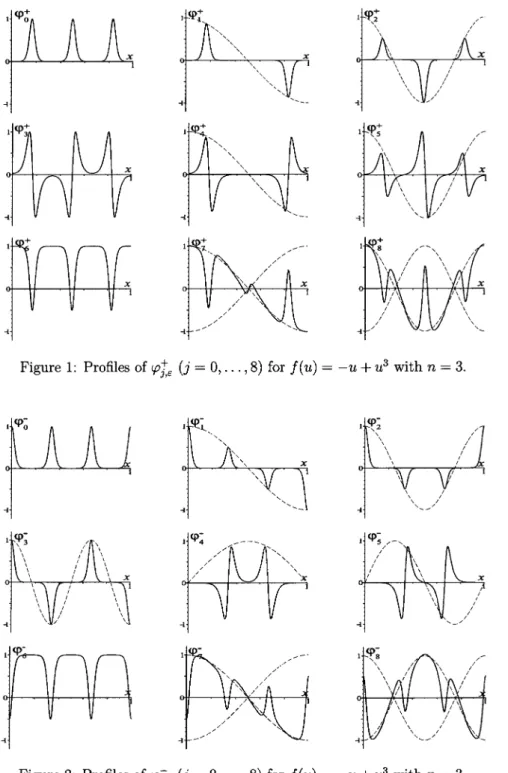
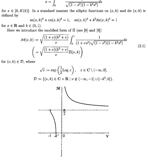
(2) 95. We are interested in the $\epsilon$‐dependence of the both eigenpairs $\lambda$_{j,$\epsilon$}^{\pm} and $\varphi$_{j,$\varepsilon$}^{\pm} for (\mathrm{L}\mathrm{P}_{\pm}) , and the qualitative difference between \{$\varphi$_{j, $\varepsilon$}^{+}\} and \{$\varphi$_{j, $\varepsilon$}^{-}\} . In the above problems we focus. on the case p=3 :. f(u)=-u+u^{3}.. In this case we can give expressions of u_{n, $\varepsilon$}^{\pm} in terms of the Jacobi elliptic function. We note that the similar expressions could be observed for the case p=2 . Moreover, the method of. representation equation, which is proposed by the author and S. Yostsutani [7], [10] and [12] for analyzing the linearized eigenvalue problems to (NP) with bistable nonlinearities, can be applied to show the precise information on eigenvalues and eigenfunctions of (\mathrm{L}\mathrm{P}_{\pm}) : \bullet. representation formulas on eigenfunctions,. \bullet. characterization of eigenvalues,. \bullet. asymptotic formulas of eigenpairs as. $\varepsilon$\rightarrow 0.. More precisely, we obtain the three special eigenfunctions for both (\mathrm{L}\mathrm{P}_{+}) and (LP‐). when p= 3 : $\varphi$_{0, $\varepsilon$}^{\pm}, $\varphi$_{0,$\varepsilon$}^{\pm} and $\varphi$_{2n, $\varepsilon$}^{\pm} . They are given explicitly in the algebraic expression of elliptic function, and also possess fine symmetric and periodic properties. Moreover,. the other eigenfunctions can be given by the Liouvillian form ([3]). The corresponding eigenvalues $\lambda$_{j,$\varepsilon$}^{\pm} of (\mathrm{L}\mathrm{P}_{\pm}) is determined by the characteristic equation,. \displaystyle \mathcal{A}(k, $\mu$)=\frac{j $\pi$}{2n}, where A is the characteristic function, which can be expressed by the complete elliptic. integral (of the third kind). The asymptotic formulas of every eigenvalue are obtained by asymptotic formulas on elliptic integrals, and the asymptotic profiles of every eigenfunction are obtained by the. Floquet / Bloch type argument with the asymptotic formulas of eigenvalues ([11] and [13]). It should be noted that in the both problem (\mathrm{L}\mathrm{P}_{\pm}) for f(u)=-u+u^{3} the three special. eigenpairs play an important role for the limit classification; every eigenpair is classified into the three classes, and roughly speaking, each class is provided by the corresponding special eigenpair. The limit classification above is described by the asymptotic formulas of eigenvalues and the asymptotic profiles of eigenfunctions when $\epsilon$ is sufficiently small. We will see that the limit classification on (\mathrm{L}\mathrm{P}_{+}) is essentially the same type as the limit. classifications for the cases of nonlinear bistable f ’s ([11] and [13]), which justify and gen‐ eralize a conjecture by E. Yanagida on the asymptotic profiles of the first n‐eigenfunctions.. The limit classification for (LP‐) will show us that Yanagida’s conjecture also hold for the first n‐eigenfunctions. However, it appears a different asymptotic characterizaton on the eigenfunctions from the case (\mathrm{L}\mathrm{P}_{+}) . which is due to the difference of the special. eigenvalues between in (\mathrm{L}\mathrm{P}_{+}) and (LP‐). See Figs. 1 and 2.. In this article we obtain the representation formulas of eigenfunctions and derive the characteristic functions for (\mathrm{L}\mathrm{P}_{\pm}) . Also, we discuss the asymtotic results on the eigen‐ values and eigenfunctions. The organization of the article is as follows. In Section 2 we prepare the elliptic integrals and functions. In Section 3 we give the main results. In Section 4 we introduce some key lemmas in the analysis and give a sketch of proofs..

(3) 96. Figure 1: Profiles of $\varphi$_{j,$\varepsilon$}^{+}. (j=0, \ldots, 8). Figure 2: Profiles of $\varphi$_{j,$\varepsilon$}^{-} (j=0,. \ldots,. for f(u)=-u+u^{3} with. n=3..

(4) 97. 2. Preliminaries. We start with giving standard notations on the elliptic integrals and elliptic functions.. See for instance, the Handbook by Byrd and Fi iedman[1]. Let k \in (0,1) and let $\nu$ \in \mathrm{C}\backslash (-\infty, -1] . We denote by K(k) , E(k) and $\Pi$(\mathrm{v}, k) , the complete elliptic integrals of the first, the second and the third kind, respectively. The Jacobi elliptic function \mathrm{s}\mathrm{n}(x, k) is a periodic analytic function with the period 4K(k) as the function for the real domain, and is defined locally by. x=\displaystyle \int_{0}^{\mathrm{s}\mathrm{n}(x,k)}\frac{1}{\sqrt{(1-s^{2})(1-k^{2}s^{2}) }ds. for x \in [0, K(k)] . In a standard manner the elliptic functions cn (x, k) and dn (x, k) is defined by. \mathrm{s}\mathrm{n}(x, k)^{2}+\mathrm{c}\mathrm{n}(x, k)^{2}=1, \mathrm{s}\mathrm{n}(x, k)^{2}+k^{2}\mathrm{d}\mathrm{n}(x, k)^{2}=1. k\in(0,1) . Here we introduce the modified form of. for x\in \mathrm{R} and. $\Pi$. (see [8] and [9]). \displaystyle \mathcal{M}( $\nu$, k):= \sqrt{\frac{(1+ $\nu$)(k^{2}+ $\nu$)}{ $\nu$} \int_{0}^{1}\frac{1}{(1+ $\nu$ s^{2})\sqrt{(1-s^{2})(1-k^{2}s^{2}) }ds. (= \sqrt{\frac{(1+ $\nu$)(k^{2}+ $\nu$)}{ $\nu$} $\Pi$( $\nu$, k). for ( $\nu$, k)\in \mathcal{D} , where. \displaystyle \sqrt{z}:=\exp(\frac{1}{2}{\rm Log} z) , z\in \mathrm{C}\backslash (-\infty, 0],. \mathcal{D}:=\{( $\nu$, k)\in \mathrm{C}\times \mathrm{R}| $\nu$\not\in(-\infty, -1]\cup[-k^{2},0. Figure 3: A Graph of \mathcal{M}( $\nu$, k) for real. \mathrm{v}(k=1/\sqrt{2}) .. (2.1).

(5) 98. 3. Main results. -u+u^{3} . A standard shooting Let us show the expressions of u_{n, $\varepsilon$}^{\pm} of (NP) for f(u) argument can be applied to (NP) (see Section 4 of [12]), and in a situation that $\epsilon$ is small enough, one can obtain the monotone increasing and decreasing solutions of (NP), which are symmetric with the line x=1/2 . In addition, one can describe the global bifurcation structue of (NP) by using the two monotone solutions. In particular, we obtain the 1/n‐periodic solutions u_{n, $\varepsilon$}^{\pm} for each n\in \mathrm{N}. =. Proposition 3.1. Fư (0,1) be a solution of. n\in \mathrm{N}. arbitrality and assume. $\varepsilon$\in. (0, \sqrt{2}/(n $\pi$)) . Let k_{ $\varepsilon$}=k_{n, $\varepsilon$}. \displaystyle \sqrt{2-k^{2} K(k)=\frac{1}{n $\varepsilon$}. \in. (3.1). (note that it is uniquely determined). Then,. u_{n,$\varepsilon$}^{+}(x)=\sqrt{\frac{2}{2-k_{$\varepsilon$}^{2} \mathrm{d}\mathrm{n}(K k_{$\varepsilon$})(1+2nx),k_{$\varepsilon$}). ,. and. u_{n,$\varepsilon$}^{-}(x)=\sqrt{\frac{2} -k_{$\varepsilon$}^{2} \mathrm{d}\mathrm{n}(2nK(k_{$\varepsilon$})x,k_{$\varepsilon$}). .. is the 1/n ‐periodic solutions of (NP) satisfying (1.1).. For a convenience, we introduce a notation of the two modified sn‐functions. \mathrm{S}\mathrm{N}^{+}(x;k)=\mathrm{s}\mathrm{n}(K(k)(1+2nx), k) , \mathrm{S}\mathrm{N}^{-}(x;k)=\mathrm{s}\mathrm{n}(2nK(k)x, k). .. Both functions have the same period 1/n for any k\in(0,1) . The functions \mathrm{C}\mathrm{N}^{\pm} and \mathrm{D}\mathrm{N}^{\pm} are defined in a similar manner;. u_{n,$\varepsilon$}^{\pm}(x)=\sqrt{\frac{2} -k_{$\varepsilon$}^{2} \mathrm{D}\mathrm{N}^{\pm}(x;k_{$\varepsilon$}). .. The representation formulas of eigenvalues and eigenfunctions are given by the follow‐ ing two theorems.. Theorem 1. The Linearized problem (\mathrm{L}\mathrm{P}_{+}) has the following pairs of eigenvalues and eigenfunctions:. (i). $\lambda$_{0,$\varepsilon$}^{+}=-1\displayst le\frac{2\sqrt{1-k_{$\epsilon$}^{2}+k_{$\varepsilon$}^{4} {2-k_{$\varepsilon$}^{2},. $\varphi$_{0, $\varepsilon$}^{+}(x)=1-(1+k_{ $\varepsilon$}^{2}-\sqrt{1-k_{ $\varepsilon$}^{2}+k_{ $\varepsilon$}^{4} )\mathrm{S}\mathrm{N}^{+}(x;k_{ $\varepsilon$})^{2}, (ii). $\lambda$_{n,$\varepsilon$}^{+}=-\displaystyle\frac{3(1-k_{$\varepsilon$}^{2}){2-k_{$\varepsilon$}^{2}f$\varphi$_{n,$\varepsilon$}^{+}(x)=\mathrm{S}\mathrm{N}^{+}(x,k_{$\varepsilon$})\mathrm{D}\mathrm{N}^{+}(x,k_{$\varepsilon$}) ,.

(6) 99. (iii). $\lambda$_{2n,$\varepsilon$}^{+}=-1+\displayst le\frac{2\sqrt{1-k_{$\varepsilon$}^{2}+k_{$\epsilon$:}^{4} {2-k_{$\varepsilon$}^{2},. $\varphi$_{2n, $\varepsilon$}^{+}(x)=-1+(1+k_{ $\varepsilon$}^{2}+\sqrt{1-k_{ $\varepsilon$}^{2}+k_{ $\varepsilon$}^{4} )\mathrm{S}\mathrm{N}^{+}(x;k_{ $\varepsilon$})^{2}, where k_{$\varepsilon$} is the unique solution of (3.1).. Theorem 2. The Lineanized problem (LP‐) has the following pairs of eigenvalues and eigenfunctions:. (i). $\lambda$_{0,$\varepsilon$}^{-}=1-\displayst le\frac{2\sqrt{1-k_{$\varepsilon$}^{2}+k_{$\varepsilon$}^{4} {2-k_{$\varepsilon$}^{2},. $\varphi$_{0, $\varepsilon$}^{-}(x)=1-(1+k_{ $\varepsilon$}^{2}-\sqrt{1-k_{ $\varepsilon$}^{2}+k_{ $\varepsilon$}^{4} )\mathrm{S}\mathrm{N}^{-}(x;k_{ $\varepsilon$})^{2}, (ii). $\lambda$_{n, $\varepsilon$2}-k^_{{-}$=\-v\aurenpsdileornl$in}^e{2{^3{f}} $\varphi$_{n, $\varepsilon$}^{-}(x)=\mathrm{C}\mathrm{N}(x, k_{ $\varepsilon$})\mathrm{D}\mathrm{N}(x, k_{ $\varepsilon$}). (iii). $\lambda$_{2n,$\varepsilon$}^{-}=1+\displayst le\frac{2\sqrt{1-k_{$\varepsilon$}^{2}+k_{$\varepsilon$}^{4} {2-k_{$\varepsilon$}^{2},. ,. $\varphi$_{2n, $\varepsilon$}^{-}(x)=-1+(1+k_{ $\varepsilon$}^{2}+\sqrt{1-k_{ $\varepsilon$}^{2}+k_{ $\varepsilon$}^{4} )\mathrm{S}\mathrm{N}^{-}(x;k_{ $\varepsilon$})^{2}, where k_{$\varepsilon$} is the unique solution of (3.1). Here we introduce the following notations. \left{bginary}l $\Lmbda_{0}(k):=-1\frc2sqt{k^}+42-{,\ $Lambd_{1}^-(k):=\frac3{2^},\ $Lambd_{1}^+(k):=-\frac31^{2})-k,\ $Lambd_{2}(k):=-1+\fracsqt{-k^2}+4 {. \endary}ight.. (3.2). Note that $\Lambda$_{0}(k)<$\Lambda$_{1}^{-}(k)<$\Lambda$_{1}^{+}(k)<0<$\Lambda$_{2}(k) for k\in(0,1) . In addition, the functions $\Lambda$_{0}, $\Lambda$_{1}^{-} and the functions $\Lambda$_{1}^{+}, $\Lambda$_{2} are monotone decreasing and increasing in k\in (0,1) , 0 and $\Lambda$_{0}(1) -3, respectively. Also, $\Lambda$_{1}(0) -2, $\Lambda$^{\pm}(0) -3/2, $\Lambda$_{2}(0) $\Lambda$_{1}^{-}(1) =. $\Lambda$_{1}^{+}(1)=0, $\Lambda$_{2}(1)=1 .. =. =. =. =. We see from Theorems 1 and 2 that. $\lambda$_{0, $\varepsilon$}^{\pm}=$\Lambda$_{0}(k_{ $\varepsilon$}) , $\lambda$_{2n, $\varepsilon$}^{\pm}=$\Lambda$_{2}(k_{ $\varepsilon$}) $\lambda$_{n, $\varepsilon$}^{-}=$\Lambda$_{1}^{-}(k_{ $\varepsilon$}) , $\lambda$_{n}^{+},\ovalbox{\t \smal REJECT}=$\Lambda$_{1}^{+}(k_{ $\varepsilon$}). ,. ,. and in particular,. $\lambda$_{0, $\varepsilon$}^{-}=$\lambda$_{0, $\varepsilon$}^{+}, $\lambda$_{+, $\varepsilon$}^{-}<$\lambda$_{n,e}^{+}, $\lambda$_{2n, $\varepsilon$}^{-}=$\lambda$_{2n, $\varepsilon$}^{+}. $\varphi$_{j,$\varepsilon$}^{\pm} .. For j\neq 0, n, 2n , let us show the representation formula of. Set. $\Sigma$_{1}^{$\Sigma$_{0} \mathrm{f}(k, $\mu$)(k, $\mu$)|k \in\in(0,1(0,1 $\mu$/(2 $\mu$/(2- k^{2})k^{2})\in\in ($\Lambda$_{1}^{+}(k),0)\}($\Lambda$_{0}(k),$\Lambda$_{1}^{-}(k) \} ,. $\Sigma$_{2} :=\{(k, $\mu$)|k\in(0,1), $\mu$/(2-k^{2})\in($\Lambda$_{2}(k), +\infty)\}.. (3.3).

(7) 100. and set. $\Sigma$:=$\Sigma$_{0}\cup$\Sigma$_{1}\cup$\Sigma$_{2}.. For (k, $\mu$)\in $\Sigma$ , the characteristic function is defined by. \mathcal{A}( $\mu$, k) :=|\mathcal{M}(\mathrm{v}_{-}(k, $\mu$), k)-\mathcal{M}($\nu$_{+}(k, $\mu$), k where. \mathcal{M}. (3.4). is defined by (2.1),. $\nu$_{\pm}(k, $\mu$):=\displaystyle \frac{3k^{2} {2}\cdot\frac{ $\mu$-3k^{2}\pm\sqrt{-3$\mu$^{2}+6(k^{2}-2) $\mu$+9k^{4} { $\mu$( $\mu$+3-3k^{2}). .. (3.5). Theorem 3. Suppose j \neq 0, n, 2n . Let k_{$\varepsilon$} be the solution of (3.1) and let $\mu$_{j}(k) be the unique solution of. where. \mathcal{A}. \displaystyle \mathcal{A}(k, $\mu$)=\frac{j $\pi$}{n} ,. (3.6). is given by (3.4). Then,. $\lambda$_{j,$\varepsilon$}^{\pm}=\displaystle\frac{$\mu$_{j}(k_{e}) 2-k_{$\varepsilon$}^{2}. Moreover,. $\varphi$_{j, \epsilon$j}^{\pm}(x)=\displaystle\sqrt{|h(u_{n,$\varepsilon$}^{\pm}(x),$\lambda$_{j, \varepsilon$}^{\pm}(k_{$\varepsilon$});k_{$\varepsilon$}\cos(\frac{1}$\varepsilon$}\int_{0}^x\frac{\sqrt{$\rho$(\lambda$_{j \epsilon$j}^{\pm},k_{$\varepsilon$}){|h(u_{n,$\varepsilon$}^{\pm}($\xi),$\lambda$_{j, \varepsilon$}^{\pm}(k_{$\varepsilon$});k_{$\varepsilon$})|d$\xi). ,. where. and. h(u, $\lambda$, k) :=-[\displaystyle \frac{k^{2} {(1+k^{2})^{2} -\frac{1}{2}u^{2}+\frac{1}{4}u^{4}] +\frac{ $\lambda$}{6}(u^{2}-2)-\frac{$\lambda$^{2} {9}. (3.7). $\rho$( $\lambda$, k)=\displaystyle \frac{1}{81}( $\lambda-\Lambda$_{0}(k) ( $\lambda-\Lambda$_{1}^{-}(k) ( $\lambda-\Lambda$_{1}^{+}(k) $\lambda$( $\lambda-\Lambda$_{2}(k) .. (3.8). Combining Theorems 1‐3 we have all eigenvalues and eigenfunctions to the both (\mathrm{L}\mathrm{P}_{+}). and (LP‐).. 4. Key lemmas on characteristic function. Proofs of Theorems 1‐3 are done by an algorithm of the representation equation for the. linearized equation of (\mathrm{L}\mathrm{P}_{\pm}) (see [12]). We would like to describe whole procedure in the. forth‐coming papers. Here we only focus on the two key lemmas for justyfing existence and uniqueness of. solution to (3.6)..

(8) 101. 4.1. Fundamental properties on the modified elliptic integral. We prepare a fundamental properties on the modified elliptic integral Proposition 4.1. Let ( $\nu$, k)\in \mathcal{D} and let \mathcal{M} be defined by (2.1). ([8] and [9]).. Then. (i). \displaystyle \frac{\partial \mathcal{M} {\partial k}( $\nu$, k)=\sqrt{\frac{(1+ $\nu$)(k^{2}+ $\nu$)}{ $\nu$} \frac{kE(k)}{(k^{2}+ $\nu$)(1-k^{2}) ,. (ii). \displaystyle \frac{\partial \mathcal{M} {\partial $\nu$}( $\nu$, k)=\sqrt{\frac{(1+ $\nu$)(k^{2}+ $\nu$)}{ $\nu$} [-\frac{K(k)}{2 $\nu$(1+ $\nu$)}+\frac{E(k)}{2(1+ $\nu$)(k^{2}+\mathrm{v}) ] (1-k^{2})K(k)<E(k)<K(k). \mathcal{M}. .. k\in(0,1) . Se we see from (ii) of Proposition 4.1 that for each k\in(0,1) the real function \mathcal{M}(\cdot, k) is decreasing for $\nu$\in(-1, k^{2})\cup(0, \infty) (see Fig. 3). Remark 4.1. It is well known that. Proposition 4.2. Fix k \in (0,1) and consider the real function (0, \infty)\rightarrow \mathrm{R} . Then the following formulas hold:. 4.2. for. \mathcal{M} (.. , k) : (-1, -k^{2})\cup. \displaystyle \lim_{ $\nu$\rightar ow-1}\mathcal{M}( $\nu$, k)=\frac{ $\pi$}{2} ,. (4.1). \displaystyle \lim_{ $\nu$\rightar ow-k^{2} \mathcal{M}( $\nu$, k)=0 ,. (4.2). \displaystyle \lim_{ $\nu$\rightar ow 0}\mathcal{M}( $\nu$, k)=\infty ,. (4.3). \displaystyle\lim_{$\nu$\rightar ow\infty}\mathcal{M}($\nu$,k)=\frac{$\pi$}{2} .. (4.4). Fundamental properties of. \mathrm{v}\pm. Recall the characteristic function. \mathcal{A}(k, $\mu$) :=|\mathcal{M}(\mathrm{v}_{+}(k, $\mu$), k)-\mathcal{M}($\nu$_{-}(k, $\mu$), k)| for (k, $\mu$)\in $\Sigma$ . We first remark that $\nu$_{\pm}(k, $\mu$) of (3.5) is characterized by. $\nu$_{+}(k, $\mu$)+$\nu$_{-}(k, $\mu$)=\displaystyle \frac{3k^{2}( $\mu$-3k^{2}) { $\mu$( $\mu$-3+3k^{2}) and. $\nu$_{+}(k, $\mu$)$\nu$_{-}(k, $\mu$)=\displaystyle \frac{9k^{4} { $\mu$( $\mu$-3+3k^{2}) . Then an elementary algebra gives. ($\nu$_{+}(k, $\mu$)-$\nu$_{-}(k, $\mu$) ^{2}=\displaystyle \frac{-27k^{4}( $\mu$-(2-k^{2})$\Lambda$_{0}(k) ( $\mu$-(2-k^{2})$\Lambda$_{2}(k) }{$\mu$^{2}( $\mu$+3-3k^{2})^{2} ..

(9) 102. Moreover, we see. \left{begin{ary}l \frac{1}$\nu_{+}(k,$\mu)}+\frac{1}$\nu_{-}(k,$\mu)}=\frac{$\mu-3k^{2}3k^{2},\ frac{1}$\nu_{+}(k,$\mu)}.\frac{1}$\nu_{-}(k,$\mu)}=\frac{$\mu($\mu+3-k^{2})9k^{4}, \end{ary}\ight. \displaytle\{ }_1^{}+\frac{}\frac{1}$\nu_{+}(k,$\mu$),\nu$_{+}(k,$\mu$)1}\{+(1\frac{1}$\nu_{-1}(k,$\mu$,(k \mu$)}(1+\frac{+}$\nu_{-}\frac{=$\mu$( \mu$}{\frac{$\mu$+3k^{2}9k^{4}+3)k^{2} \displaystle\{ }_1^{}+\frac{}+\frac{k^2}{$\nu$_{+}(k,$\mu$),\nu$_{+}(k,$\mu$)k^{2}\+(1\frac{k^2}{$\nu$_{-}(k,$\mu$,(k \mu$)k^{2})(1+\frac{+}$\nu$_{-}\frac{=\frac{$\mu$+6-3k^{2}+3)($\mu$+3k^{2}($\mu$-3k^{2})9 , ,. and. respectively.. (4.5). (4.6). (4.7). The following proposition helps some calculations on the characteristic functions to‐ gether with M.. Proposition 4.3. For $\nu$_{\pm}=$\nu$_{\pm}(k, $\mu$) of (3.5). \displaystyle \frac{1}{ $\nu$\pm}(1+\frac{1}{ $\nu$\pm}) (1+\frac{k^{2} { $\nu$\pm}) =\frac{ $\mu$( $\mu$-3)( $\mu$+3-3k^{2}) {27k^{4} . 4.3. Several limit for characteristic function. Lemma 4.1. Let. k\in. (0,1) be fixed and (k, $\mu$). \in $\Sigma$ .. Then the following (i) and (ii) hold. true:. (i). \displaystyle \lim_{ $\mu$\rightar ow(2-k^{2})$\Lambda$_{0}(k)}\mathcal{A}(k, $\mu$)=0, \displaystyle \lim_{ $\mu$\rightar ow-3}\mathcal{A}(k, $\mu$)=\frac{ $\pi$}{2}.. (ii). \displaystyle \lim_{ $\mu$\rightar ow-3(1-k^{2}) \mathcal{A}(k, $\mu$)=\frac{ $\pi$}{2},. \displaystyle \lim_{ $\mu$\rightar ow 0}\mathcal{A}(k, $\mu$)= $\pi$.. Proof of Lemma 4.1. (i) Suppose that (k, $\mu$)\in$\Sigma$_{0} . Then, it follows from (4.5)-(4.7) that. -1<$\nu$_{-}(k, $\mu$)<$\nu$_{+}(k, $\mu$)<-k^{2} \bullet. \bullet. and. \displaystyle \lim_{ $\mu$\rightar ow(2-k^{2})$\Lambda$_{0}(k)}$\nu$_{\pm}(k, $\mu$)=\mathrm{v}_{*}(k)\in(-1, k^{2}). ,. \displaystyle \lim_{ $\mu$\rightar ow-3}$\nu$_{-}(k, $\mu$)=-1, \displaystyle \lim_{ $\mu$\rightar ow-3}$\nu$_{+}(k, $\mu$)=-k^{2}.. Therefore, by using monotonicity of \mathcal{M}. \displaystyle \lim_{ $\mu$\rightar ow(2-k^{2})$\Lambda$_{0}(k)}\mathcal{A}(k, $\mu$)= \lim_{ $\mu$\rightar ow(2-k^{2})$\Lambda$_{0}(k)}(\mathcal{M}($\nu$_{-}(k, $\mu$), k)-\mathcal{M}(\mathrm{v}_{+}(k, $\mu$), k) =\mathcal{M}(\mathrm{v}_{*}(k), k)-\mathcal{M}(\mathrm{v}_{*}(k), k) =0..

(10) 103. In the similar manner we see from (4.1) and (4.2) of Proposition 4.2 that. \displaystyle \lim_{ $\mu$\rightar ow-3}\mathcal{A}(k, $\mu$)= \lim_{ $\mu$\rightar ow-3}(\mathcal{M}($\nu$_{-}(k, $\mu$), k)-\mathcal{M}($\nu$_{+}(k, $\mu$), k)) =(\mathcal{M}(-1, k)-\mathcal{M}(-k^{2}, k)) =^{\underline{ $\pi$} 2. Thus it complete a proof. \square. (ii) of the lemma is similarly done. So we omit it.. Previous results for the cases of bistable nonlinearities suggest that we will also have. (iii). \displaystyle \lim_{ $\mu$\rightar ow(2-k^{2})$\Lambda$_{2}(k)}\mathcal{A}(k, $\mu$)= $\pi$.. However, a different type of asymptotic formulas should be applied to show the above claim. So we omit it.. 4.4. Monotonicity of characteristic function. Lemma 4.2. Let (k, $\mu$)\in $\Sigma$ . For each. i=0 ,. 1, 2,. \displayst le\frac{\partial\mathcal{A}{\partial$\mu$}(k,$\mu$)>0. in $\Sigma$_{i}.. Proof. Denote $\nu$_{\pm}:=\mathrm{v}_{\pm}(k, $\mu$) and set. \displaystyle \mathcal{R}(k, $\mu$):=\frac{ $\mu$( $\mu$-3)( $\mu$+3-3k^{2})}{27k^{4} . For simplicity we only consider the case (k, $\mu$)\in$\Sigma$_{0} . By using (ii) of Proposition 4.1 and Proposition 4.3, we are led to. \displayst le\frac{\parti l\mathcal{A}{\parti l$\mu$}=\frac{\parti l\mathcal{M}{\parti l$\nu$}( \nu$_{-},k)\cdot\frac{\parti l$\nu$_{-} \parti l$\mu$}-\frac{\parti l\mathcal{M}{\parti l$\nu$}( \nu$_{+},k)\cdot\frac{\parti l$\nu$_{+}{\parti l$\mu$} =. \displaystyle \sqrt{\frac{(1+$\nu$_{-})(k^{2}+$\nu$_{-}) {$\nu$_{-} [-\frac{K(k)}{2$\nu$_{-}(1+$\nu$_{-}) +\frac{E(k)}{2(1+$\nu$_{-})(k^{2}+$\nu$_{-}) ] \displayte\frac{ptial$\nu_{-}\partil$\mu} -\displaystyle \sqrt{\frac{(1+$\nu$_{+})(k^{2}+$\nu$_{+}) { $\nu$+} [-\frac{K(k)}{2$\nu$_{+}(1+$\nu$_{+}) +\frac{E(k)}{2(1+$\nu$_{+})(k^{2}+$\nu$_{+}) ] \displayte\frac{prtial$\nu_{+}\partil$\mu} .. .. = \displaystyle \sqrt{\mathcal{R}(k, $\mu$)}(-$\nu$_{-}\frac{\partial$\nu$_{-} {\partial $\mu$}) [-\frac{K(k)}{2$\nu$_{-}(1+$\nu$_{-}) +\frac{E(k)}{2(1+$\nu$_{-})(k^{2}+$\nu$_{-}) ] -\displaystyle \sqrt{\mathcal{R}(k, $\mu$)}(-$\nu$_{+}\frac{\partial $\nu$+}{\partial $\mu$}) [-\frac{K(k)}{2$\nu$_{+}(1+$\nu$_{+}) +\frac{E(k)}{2(1+$\nu$_{+})(k^{2}+$\nu$_{+}) ]. =\displaystyle\frac{\sqrt{\mathcal{R}(k,$\mu$)}{2}[(\frac{1}{1+$\nu$_{-}\frac{\partial$\nu$_{-}{\partial$\mu$}-\frac{1}{1+$\nu$+}\frac{\partial$\nu$+}{\partial$\mu$})K(k) -(\displaystyle\frac{$\nu$_{-}{(1+$\nu$_{-})(k^{2}+$\nu$_{-})\frac{\partial$\nu$_{-}{\partial$\mu$}-\frac{$\nu$+}{(1+$\nu$_{+})(k^{2}+$\nu$_{+})\frac{\partial$\nu$+}{\partial$\mu$})E(k)].

(11) 104. and furthermore,. \displayst le\frac{\partial\mathcal{A}{\partial$\mu$}(k, $\mu$)=\frac{1}2\sqrt{\mathcal{R}(k,$\mu$)}[(\frac{k^2}+$\nu$_{-} $\nu$^{\underline{3} \frac{\partial$\nu$_{-} \partial$\mu$}-\frac{k^2}+$\nu$_{+}{$\nu$_{+}^{3}\frac{\partial$\nu$_{+}{\partial$\mu$})K(k) -(\displaystle\frac{1}$\nu$^{\underline{2} \frac{\partil$\nu$_{-} \partil$\mu$}-\frac{1}$\nu$_{+}^2}\frac{\partil$\nu$_{+} \partil$\mu$})E(k)] =\displaystyle\frac{1}{2\sqrt{\mathcal{R}(k,$\mu$)} [\frac{\partial}{\partial$\mu$}[(\frac{1}{$\nu$_{+} -\frac{1}{$\nu$_{-} )(1+\frac{k^{2} {2}(\frac{1}{$\nu$_{+} +\frac{1}{l\text{ノ_{-} ) ]K(k) -\displaystyle\frac{\partial}{\partial$\mu$}(\frac{1}{$\nu$_{+}-\frac{1}{$\nu$_{-})E(k)] =\displaystyle \frac{S_{1}(k,$\mu$)K(k)+S_{2}(k,$\mu$)E(k)}{6k^{2}\sqrt{\mathcal{R}(k,$\mu$)}\sqrt{-3$\mu$^{2}+6(k^{2}-2) $\mu$+9k^{4} ,. where. S_{1} :=$\mu$^{2}+3(2-k^{2}) $\mu$+6(1-k^{2}) , S_{2} :=-3( $\mu$-k^{2}+2). .. Finally, the claim of the lemma is proved by repeating argument in [12, Proof of Lemma \square 6.2].. References [1] P.. $\Gamma$ .. Byrd and M. D. Friedman, “Handbook of Elliptic Integrals for Engineers and. Scientists. Springer‐Verlag, 1981.. [2] H. Berestycki and P.‐L. Lions, Nonlinear scalar field equations I: existence of a ground state, Arch. Rational Mech. Anal., 82 (1983), 313‐345. [3] J. Kovacic, An algorithm for solving second order linear homogeneous differential equations, J. Symbolic Comput., 2 (1986), 3‐43.. [4] C.‐S. Lin, W. Ni and I. Takagi, Large amplitude stationary solutions to a Chemotaxis system, J. Differential equations, 72 (1988), 1‐27. [5] Y. Miyamoto and K. Yagasaki, Monotonicity of the first eigenvalue and the global bifurcation diagram for the branch of interior peak solutions, J. Differential equations,. 254 (2013), 342‐367.. [6] K. Takemura, The Heun equation and the Calogero‐ Moser‐Sutherland system I: the Bethe Ansatz method, Commun. Math. Phys. 235 (2003), 467‐494. [7] T. Wakasa, Exact eigenvalue and eigenfunction associated with linearization for Chafee‐Infante problem, Funkcialaj Ekvacioj, 49 (2006), 321‐336. [8] T. Wakasa, Note on parameter dependence of eigenvalues for a linearized eigenvalue problem, Bull. Kyushu Inst. Tech., 49 (2016), 1‐12..

(12) 105. [9] T. Wakasa, Analysis on the linearized eigenvalue problems and its application the global bifurcation problems, Lecture note on “Study meeting on Applied Mathematics. 2016”’ (Japanese).. [10] T. Wakasa and S. Yotsutani, Representation formulas for some 1‐dimensional lin‐ eaMed eigenvalue problems, Commun. Pure Appl. Anal. 7 (2008), 745‐763. [11] T. Wakasa and S. Yotsutani, Asymptotic profiles of eigenfunctions for some 1‐ dimensional linearized eigenvalue problems, Commun. Pure Appl. Anal. 9 (2010). [12] T. Wakasa and S. Yotsutani, Limiting classification on linearized eigenvalue prob‐ lem for 1‐dimensional Allen‐Cahn Equation I ‐Asymptotic formulas of eigenvalues J.. Differential equations, 258 (2015), 3960‐4006. [13] T. Wakasa and S. Yotsutani, Limiting classification on lineart,zed eigenvalue problem for 1‐dimensional Allen‐Cahn Equation II ‐Asymptotic profiles of eigenfunctions J.. Differential equations, 261 (2016), 5465‐5498.. [14] E. T. Whittaker and G. N. Watson, “A Course of Modern Analysis“, Fourth Edition, Cambridge University Press, New York, (1962)..

(13)