Structural Induction and the $\lambda$-Calculus (Algebra, Logic and Geometry in Informatics)

Structural

Induction and the

A-Calculus

Rene’ Vestergaard*

School of InformationScience

JapanAdvanced Institute ofScienceandTechnology

Abstract. We consider formal

provabil-ity with structural induction and related

proof principles in the $\lambda$-calculus presented

with first-0rder abstract syntax over

one-sorted variable names. As well as

sum-marising and elaborating on earlier,

for-mally verified proofs (in $\mathrm{I}\mathrm{s}\mathrm{a}\mathrm{b}\mathrm{e}\mathrm{l}\mathrm{l}\mathrm{e}/\mathrm{H}\mathrm{O}\mathrm{L}$) of the relative renaming-freeness of $\beta-$ residual theory and $\beta$-confluence, we also present proofs of$\eta$-confluence,$\beta\eta-$-confluence,

the strong weakly-finite $\beta$-development(aka

residual-completion) property, residual $\beta-$

confluence $\eta-\mathrm{o}\mathrm{v}\mathrm{e}\mathrm{r}-\beta$-postponement, and no

tably$\beta$-standardisation.Inthelatter case,the

known proofs fail in instructiveways.

Interest-ingly, our uniform proof methodology, which

has relevance beyond the A-calculus, proof

erlycontains pen-and-paper proof practices in

aprecise sense. The proofmethodology also

makes precisewhat isthe fullalgebraic proof

burden of the considered results, which we, moreover, appear to be the first to resolve.

1Introduction

The use of structural induction and related proof

prin-ciplesfor simple syntax (i.e.,first-0rderabstract syntax

over one-sorted variable names) is along-standing and

widely-usedpracticein the programming-language

the-orycommunity.Unfortunately, atafirst, closer inspec-tion it seems that the practice is not formally

justifi-able because of aneed to avoid undue varijustifi-able capture when performing substitution, thus breaking the

syntac-tic equality underlying structural induction, etc.. Even

more

worrying is the fact that, in spite of substantial

efforts in themechanised theorem-proving community,

no

formal proof developments (priortowhat

we

report

onhere) have been able to

overcome

the problems that

are

encountered with substitution andgoonto

success-fully employ the proof principles in question. Indeed,

and starting with de Bruijn [6], it has becomeanactive

research

area

to define, formalise, and automate

alter-native syntactic frameworks that,onthe

one

hand,

pre-serve

asmuch ofthe inherentnaturalityof simplesyntax

as possible. At the same time, they are customised to

provide suitable induction and recursion principles for

any considered language [6-10,12, 17,21]. However, by

changing the underlyingsyntacticframework, the

alge-braic meaningof,$\mathrm{e}.\mathrm{g}.$,adiamond property also changes,

which

means

that, e.g., confluence as provedandasde

finedno longercoincide, cf.Lemma 18 and [25].

In the recognition that the above is both

unfortu-nateasfarastheformal status of the existing informal

literature isconcerned andunsatisfactoryfrom

amath-ematical Perspective, we pursue the naive approach in

this article (while incorporating the relevant aspects of

$[24, 25])$

.

In particular, we show that it is, indeed, pos

sible to base formal proofs on first-0rder abstract

syn-tax over one-sorted variable

names

and hope to

con-vince the reader that, while the technical gap between

pen-and-paper and formal proofs is rather large, the

conceptual gap is somewhat smaller. Furthermore, we

hope that the comprehensive range of applications of

the proof methodology that wepresent here will estab

lish its widerrelevance.

1.1 Syntax ofthe A-Calculus

The A-calculus is intended to capture the concept of

afunction.

It does so, first ofall, by providing syntax

that can be used to express function application and

definition:

$e::=x$ $|e_{1}e_{2}|$ Xx.$\mathrm{e}$

The above, informal syntax says that aA-term, $e$,

is defined inductively

as

either avariable name,

as an

application of

one

term to another,

or

as a$\lambda-$,

or

func-tional, abstraction of avariable

name

over aterm. The

variable names, $x$,

are

typically taken to be, or range

over, words

over

the Latin alphabet. In Section 2, we

willreview the exactrequirementsto variable

names

in

an abstract

sense.

Being based on asimple, inductive

definition, A-terms also

come

equipped with arange of

primitive proofprinciples $[1, 3]$

.

Syntactic Equality As aA-term, $e$, is finite and

con-sistsofvariable names, the obvious variable

name

equal-ity, $=vN$, which exists at least in the caseofwords

over

the Latin alphabet, canonically extends to all A-terms:

$\underline{x=vNy}e_{1\Lambda^{\mathrm{v}\mathrm{a}\mathrm{r}}}=e_{1}’$ e2 $=\Lambda^{\mathrm{v}\mathrm{a}\mathrm{r}}e_{2}^{J}x=vNye=\Lambda^{\mathrm{v}u}e’$

$x$$=_{\Lambda^{\mathrm{v}\mathrm{a}\mathrm{r}}}y$ $e_{1}e_{2}=_{\Lambda}\mathrm{v}-\mathrm{r}e_{1}’e_{2}’$ $\overline{\lambda z.e=_{\Lambda^{\mathrm{v}\mathrm{a}\mathrm{r}}}\lambda y.e^{l}}$

Structural Induction In order to prove properties

about theset of A-terms,

we can

proceed by means of

structural induction, mimicking the inductivedefinition

of the terms:

Vz.P(z)$\forall e_{1}$,$e_{2}.P(e_{1})\Lambda P(e_{2})\Rightarrow P(e_{1}e_{2})\forall x$,$e.P(e)\Rightarrow \mathrm{P}(\mathrm{X}\mathrm{x}.\mathrm{e})$ $\star$

vester@jaist.ac.jp, http:$//\mathrm{w}\mathrm{w}\mathrm{w}.\mathrm{j}$aist.ac.j$\mathrm{p}/$-vester Ve.P(e)

数理解析研究所講究録 1318 巻 2003 年 30-45

$y[x\cdot=e]_{\mathrm{C}\mathrm{u}}=\{$

$e$ if$x=y$

$y$ otherwise $(e_{1}e_{2})[x:=e]\mathrm{c}_{\mathrm{u}}=e_{1}[x:=e]_{\mathrm{C}\mathrm{u}}e_{2}[x:=e]_{\mathrm{C}\mathrm{u}}$

$(\lambda y.e\mathrm{o})[x:=e]_{\mathrm{C}\mathrm{u}}=\{$

$\lambda y.e0$ if_$x=y$

Xx.eo$[x:=e]\mathrm{c}\mathrm{u}$ if$x\neq y\wedge(y\not\in \mathrm{F}\mathrm{V}(\mathrm{e})\vee x\not\in \mathrm{F}\mathrm{V}(e_{0}))$

$\lambda z.e\mathit{0}[y:=\mathrm{z}]\mathrm{c}\mathrm{n}[\mathrm{x} :=e]\mathrm{c}_{\mathrm{u}}$ $0/\mathrm{W}j$

first

$z\not\in\{x\}\mathrm{U}\mathrm{F}\mathrm{V}(\mathrm{e})\mathrm{U}\mathrm{F}\mathrm{V}(e_{0})$

Fig.1. Curry-style capture-avoiding substitution

x

_I

y $e_{1}[x :=e]\mathrm{c}_{\mathrm{u}}=e_{1}’$ e2[x$:=e]\mathrm{c}\mathrm{u}=e_{2}’$

$x[x :=e]_{\mathrm{C}\mathrm{u}}=e$ $y[x:=e]\mathrm{c}_{\mathrm{u}}=y$ (eie2)[x$:=e$]$\mathrm{C}\mathrm{u}e’1=e’2$

$x\neq y$ $(y\not\in \mathrm{F}\mathrm{V}(\mathrm{e})\vee x \not\in \mathrm{F}\mathrm{V}(e_{0}’))$ $\mathrm{e}\mathrm{o}[\mathrm{x}:=e]\mathrm{c}_{\mathrm{u}}=e_{0}^{\mathit{1}}$

$(\lambda x.e\mathrm{o})[x:=e]\mathrm{c}_{\mathrm{u}}=\lambda x.eo$ (Xy.eo)[x_$:=e$]$\mathrm{c}_{\mathrm{u}}=\lambda y.e_{0}’$

$z\neq yy\in \mathrm{F}\mathrm{V}(e)x\in \mathrm{F}\mathrm{V}(eo)z=\mathrm{F}\mathrm{r}\mathrm{e}\mathrm{s}\mathrm{h}((e_{0}e)x)\mathrm{e}_{0}[\mathrm{y}:=z]\mathrm{c}_{\mathrm{u}}=e_{0}’e_{0}’[x:=e]\mathrm{c}_{\mathrm{u}}=e_{0}’$

$(\lambda y.e\mathrm{o})[x:=e]_{\mathrm{C}\mathrm{u}}=\lambda z.e_{0}’$

Fig.2. Curry-style substitution (re-)defined inductively

Structural Case-Splitting As each syntax

construc-torof theA-calculusis unique, we seethat it is possible

to

case

splitonterms –with$E_{\dot{1}}$ insome suitable meta

language:

case$e$ of $x\Rightarrow E_{1}(x)$

$|$ $e_{1}e_{2}\Rightarrow E_{2}(e_{1}, e_{2})$

$|\lambda x.e_{0}\Rightarrow E_{3}(x, e_{0})$

Structural Recursion Based on case-splitting and

well-foundedness ofterms,we can even define functions

on A-terms by

means

of structural recursion, i.e., by

making recursive calls only onthe subterms of agiven

constructor:

$f(x)=E_{1}(x)$

$f(e_{1}e_{2})=E_{2}(f(e_{1}), f(e_{2}))$

$f(\lambda x.e)=E_{3}(x, f(e))$

The above implies that $f$ is well-defined: it is

com-putable by virtue ofwell-foundedness ofterms and to

talbecausethe definitioncase-splits exhaustivelyon $\lambda-$

terms. Asanexample application,wedefine the function

that computes the

_free

variables inaterm, i.e., the

vari-able$\mathrm{n}$

ames

that do not

occur

inside aA-abstraction of

themselves. Definition 1

$\mathrm{F}\mathrm{V}(y)=\{y\}$

$\mathrm{F}\mathrm{V}(e_{1}e_{2})=\mathrm{F}\mathrm{V}(\mathrm{e})\mathrm{U}\mathrm{F}\mathrm{V}(\mathrm{e})$

$\mathrm{F}\mathrm{V}(\lambda y.e)=\mathrm{F}\mathrm{V}(\mathrm{e})\backslash \{y\}$

Proposition 2 $\mathrm{F}\mathrm{V}(-)$ isatotal,computable

function.

1.2 Reduction and Substitution

In order to haveA-abstractions actasfunctions andnot

tohave too many,e.g.,identityfunctions, amongstother

things, we are typically interested in the following rela

tions that can be applied anywhere in aterm –their

preciseform is dueto Curry [4].

1. $(\lambda x.e)e’$ – $,\beta^{\mathrm{c}_{\mathrm{u}}e[x:=e’]\mathrm{c}_{\mathrm{u}}}$

2. $\lambda y.e[x:=\mathrm{y}]\mathrm{C}\mathrm{u}--*_{\alpha^{\mathrm{C}\mathrm{u}}}$ Xx.e, if y $\not\in \mathrm{F}\mathrm{V}(e)$

Our interest in 2., above is the equivalence relation it

induces. We denote it by $==_{\alpha}$, cf. Appendix $\mathrm{B}$, and we

will eventually factor itout, asis standard.

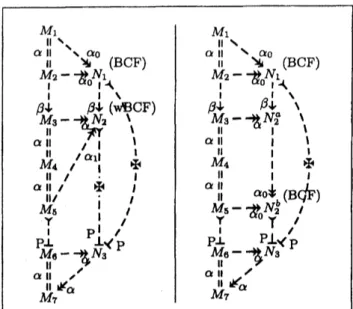
Variable Capture In his seminal formalist

presenta-tionof theA-calculus[4], Curry defines the above

substi-tution operator, $-[-:=-]_{\mathrm{C}\mathrm{u}}$,essentially

as

in Figure1.

The lastclause is the interestingone.It

renames

the

con-sidered$y$intothefirst$z$that has not been used already.1

Consider, for example, thesubstitutionof$x$for$z$inthe

twoterms Xx.z and Xy.z. Both terms-as-functions

dis-card their argument. If

we

simply replace the $z$ in the

terms with$x$,thelatterwouldstilldiscard its argument

but the formerwouldbecome the identity function and

this discrepancy would lead to inconsistencies.

Well-Definedness Of formalist relevance, we remark

that Curry-style substitution is notwell-definedby

con-struction as the definition does not employ structural

1 _{While thenotion “the first} $z$”is triviallywell-defined in

the presentcase,the issueis abitmoresubtleinawider

context,as weshallseein Section 2.

recursion. The offender is the last clause that applies $-[x:=e]$to aterm, $e_{0}[y:=z]$,which is notasubtermof

$\lambda y.e_{0}$ ingeneral. It

can

be observed that while$e0[y:=z]$

is not asub term of Ay.eo, it will have the same size

as $e_{0}$ and we can thus establish the well-formedness of

$-[-:=-]\mathrm{c}_{\mathrm{u}}$ by external

means.

Alternatively, we

can

introduce amore advanced, parallel substitution

oper-ator [22]. However, as we eventually will distance

our-selves ffom the useof renaming in substitution, we will

do neither but instead refer toSection 2.3 foran

alter-nativederivation of Curry-style substitution.

variableName Indeterminacy Having initially

committed ourselves tousing renaming in substitution,

arange

ofproblems

are

brought down

on us.

Hindley

[11] observed, for example, that it becomes impossible

to predict the variable name used for agiven

abstrac-tion afterreducing, thus putting,e.g., confluence out of reach:

$–*\beta^{\mathrm{C}\mathrm{u}}(\lambda y.\lambda x.zy)y--arrow\lambda x.xy\beta^{\mathrm{C}\mathrm{u}}$

$(\lambda x.(\lambda y.\lambda x.xy)z)y--\beta^{\mathrm{C}\tilde{\mathrm{u}}}(\lambda x.\lambda z.zx)y--arrow\lambda z.zy$

$\beta^{\mathrm{C}\mathrm{u}}$

In the lower branch, the innermost $x$abstraction must

berenamed to a$z$-abstraction, whilethe upper branch

neverencounters the variablename clash. Hindley pro

ceeded to define a $\beta$-relation

on

$\alpha$-equivalence classes

that

overcomes

the above indeterminacy by factoring it

out:

$\lfloor e\rfloor=^{\mathrm{d}\mathrm{e}t}\{e’|e==_{a}e’\}$

$\lfloor e_{1}\rfloorarrow\beta^{\mathrm{H}1}\mathrm{L}e_{2}\rfloor=^{\mathrm{d}\mathrm{e}\mathrm{f}}\exists e_{1}’\in\lfloor e_{1}\rfloor,e_{2}’\in\lfloor e_{2}\rfloor.e’1--mathrm{c}_{\mathrm{u}}\beta e_{2}’$

No relevant proof principles

are

introduced by this

and the approachcannot be used in aformal settingas

itstands.

Broken Induction Steps Instead of factoring out

a-equivalence altogether, one could attempt to

reason

up to post-fixed

name

unification. Unfortunately, this

would leadtoarangeofunusual situations asfaras sub

sequentusesof abstract rewriting is concerned. An

ex-aanpleis thefollowingattempted adaptation of the

well-knownequivalencebetween confluenceand the

Church-Rosserproperty.Please refer to Appendix Afor aprecise

definition ofourdiagram notation.

Non-Lemma 3

$..\swarrow.[searrow] \mathrm{h}4_{arrow}\acute{.}l$

.

$\Rightarrow$

$.\backslash ,-_{\mathrm{v}\backslash }-_{u’}\backslash \mathrm{A}’\mathrm{O}*\wedge\backslash \wedge\cdot \mathrm{O}’ J^{\cdot}$

$0^{\wedge\wedge\prime}$ $\wedge$

$0$

Proof (pSlLS) Byreflexive, transitive,$\mathrm{s}\mathrm{y}\mathrm{m}\mathrm{m}\mathrm{e}\mathrm{t}\mathrm{r}\mathrm{i}\mathrm{c}\alpha$

in-Section in $=$

.

Base, Reflexive, Symmetric Cases: Simple.

Transitive Case: Breaks down.

Broken a-Equality in Sub-Terms Havingfailed in

our

attempts to control limited use of a-equivalence,

one

might think that the syntactic version of Hindley’s

approach, cf. Section 1.2, could work: that it is possible

to stateall properties about terms_uPto$==_{\alpha}$rather than

the primitive$=\Lambda^{\mathrm{V}\mathrm{A}}$.

Lemma4(Simplified Substitution modulo $\alpha$)

$e_{1}==_{\alpha}$ e2$\Lambda x\neq y.\cdot$$\Lambda y_{1}\neq y_{2}$

$\Downarrow$

$e_{1}[x_{1}:=y_{1}]_{\mathrm{C}\mathrm{u}}[x_{2}:=y\mathrm{z}]_{\mathrm{C}\mathrm{u}}-=_{\alpha}e_{2}[x_{2}:=y_{2}]_{\mathrm{C}\mathrm{u}}[z_{1}:=y_{1}]_{\mathrm{C}\mathrm{u}}$

Proof (FAILS) By structural induction in $e_{1}$

.

Most Cases: Trivial.

Last Abstraction Case (simplified): Breaks down.

$(\lambda y_{1}.e)[x_{1}:=y_{1}]_{\mathrm{C}\mathrm{u}}[x_{2}:=y_{2}]$

$=\lambda z.e’[x_{1}:=y_{1}]_{\mathrm{C}\mathrm{u}}[x_{2}:=y_{2}]_{\mathrm{C}\mathrm{u}}$

$==_{\alpha}^{\mathrm{f}\mathrm{f}}\lambda z.e’[x_{2}:=y_{2}]_{\mathrm{C}\mathrm{u}}[x_{1}:=y_{1}]_{\mathrm{C}\mathrm{u}}$

$=(\lambda z.e’)[x_{2}:=y_{2}]_{\mathrm{C}\mathrm{u}}[x_{1}:=y_{1}]_{\mathrm{C}\mathrm{u}}$

The problem above is that$e$and$e’$arenotactually$\alpha-$

equivalent,

even

if$\lambda y_{1}.e$and$\lambda z.e’$are, and the$==_{\alpha}$-step

canthus not be substantiated by the induction

hypoth-esis. Consider, e.g.,$e$as$y_{1}$and$e’$ae $z$

.

Theabove result

is certainlycorrectbut,unfortunately, not provable with

thetools

we

have at ourdisposal at themoment

1.3 This article

The results we are dealing with are mostly well-known

and have been addressed in several contexts. Indeed, a

number oftruly beautiful and concise informal proofs

exist;see, in particular, Takahashi [23], whomwe owe a

great debt. This article, therefore, spends little energy

onthosepartsof the proofs and focuses instead on what

it takes to formalise them. Therearetwo keyissues: (i)

thesyntactic properties thatcanactuallybeestablished

uP to $=_{\Lambda^{\mathrm{v}*\mathrm{r}}}$ (asopposedto $==_{\alpha}$, which wehave seento

be highlyproblematic) and (ii) howto generalise these

tothe algebraic propertieswe

are

seeking. The full type

set proofs (roughly 100 pages for the proofs alone) are

available fiiomour homepage.

In general, our proofs follow the structure that we

present in Figure3. It is based

on

nestedinductions.The

full-coloured arrowsmean “is the key lemma for”, while

the othersmean “is used tosubstantiateside addition

on lemma applications”. The first issue above, (i), is

expressedintheaddition of the “Variable Monotinicity”

prooflayer inFigure3. The secondissue, (ii),isentirely

accounted for in the “Administrative ProofLayer” in

Figure 3.

The proofs underpinning Sections 3and 4.1 have been

verified in full in$\mathrm{I}\mathrm{s}\mathrm{a}\mathrm{b}\mathrm{e}\mathrm{l}\mathrm{l}\mathrm{e}/\mathrm{H}\mathrm{O}\mathrm{L}$(at least in the case of

one of the alternatives they present) $[24, 25]$

.

By the

natureof Figure 3, this

means

that substantial parts of

the other proofs essentiallyhave been verifiedas well.

Apartfrom the various technical sections in the body

ofthis paper, the appendix section contains an expla

nation ofour diagramnotation (Appendix A) and our

other notation(Appendix B)aswellas somewell-known

rewritingresults thatwe

use

(Appendix$\mathrm{C}$).

2The

$\mathrm{A}^{\mathrm{v}\mathrm{a}\mathrm{r}}$

-Calculus

Having

seen

that the standard presentations of the $\lambda-$

calculus lead toformalist problems,wewillnowgive an

alternative presentation that

overcomes

them. The

dif-ferent presentations differ only in how they lend

them-selves to provability. Their equational properties

are

equivalent.

2.1 Formal Syntax

Weuse $e’ \mathrm{s}$ to range

over

the inductively built-up set of

A-terms.The variablenames,$\mathcal{V}N$, aregeneric butmust

meet certain minimal requirements.

Definition 5 $\Lambda^{\mathrm{v}\mathrm{a}\mathrm{r}}::=VN$

$|\Lambda^{\mathrm{v}\mathrm{a}\mathrm{r}}\Lambda^{\mathrm{v}\mathrm{a}\mathrm{r}}|\lambda \mathcal{V}N.\Lambda^{\mathrm{v}\mathrm{a}\mathrm{r}}$

Assertion 6 $\mathcal{V}N$ is asingle-sorted set

of

objects, aka

variable

names.

Assertion 7 $\mathcal{V}N- equal_{i}ty_{l}=vN$, is decidable.

Assertion 8There exists

a

total, computable

func-tion, Fresh(-): $\Lambda^{\mathrm{v}\mathrm{a}\mathrm{r}}arrow \mathcal{V}N$, such$that^{\mathit{2}}$

.

besh(e)\not\in FV(e)U$\mathrm{B}\mathrm{V}(e)$

The last assertion trivially implies that$\mathcal{V}N$is infinite.3

We shalluse$x’ \mathrm{s}$,$y’ \mathrm{s}$, and$z’ \mathrm{s}$asmetavariable of$\mathcal{V}N$

and, by aslight abuse ofnotation, also

as

actual

vari-ablenamesinterms. We will suppress the$\mathcal{V}N$suffixon

variable-name equality andmerely write, e.g., $x$_$=y$.

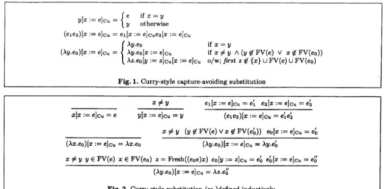
2.2 Orthonormal Reduction

The key technicalitytoprevent implicit renaming is

our

useof apredicate,$\mathrm{C}\mathrm{a}\mathrm{p}\mathrm{t}_{x}(e_{1})\cap \mathrm{F}\mathrm{V}(e_{2})=\emptyset$,cf. Figure 4,

whichguaranteesthat

no

capturetakes place in thesub

stitution: $e_{1}[x :=e_{2}]$. Itcoincides with the notion of not

free for.

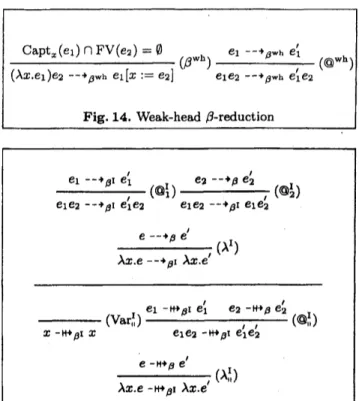
Definition 9(The $\lambda^{\mathrm{v}\mathrm{a}\mathrm{r}}$ Calculus) The terms

of

the

$\lambda^{\mathrm{v}\mathrm{a}\mathrm{r}}$-calculus are $\Lambda^{\mathrm{v}\mathrm{a}\mathrm{r}}$,

cf. Definition

5. The (indexed) $\alpha-$, $\beta-$, and

$\eta$-reduction relations

of

$\lambda^{\mathrm{v}\mathrm{a}\mathrm{r}}$: _$-*:\alpha-$,

$–*\rho$,

and $–*_{\eta}$ are given inductively in Figure 5. The plain

$Ct$-relationis:

$e–*_{\alpha}e’\Leftrightarrow^{\mathrm{d}\mathrm{e}\mathrm{f}}\exists y.e-^{y}\_{i\alpha}e’$

Unlike the situationwithCurry-style substitution,

we

see that

our

notion of substitution is defined by

struc-tural recursion and, hence, iswell-defined by construc-them.

Proposition 10 $-[x:=e]$ isatotal, computable

func-them.

2_{Forthedefinitionof BV(-),seeFigure4.}

3 _{Inthesettingof NominalLogic [19],theassertion also}

val-idatestheaxiom ofchoice,whichisknowntobe provably

inconsistentwiththeFraenkel-Mostowski settheorythat

underpins Nominal Logic. Nominal Logic instead

guar-antees the existence ofsome fresh variable name, which

by design can be any variable name except for afinite

number. Morework needs to be done to clarifythe

cor-respondence betweensimple syntax andsyntaxbased on

Nominal Logic.

$y[x:=e]=\{$_{y otherwise}eif x$=y$

$(e_{1}e_{2})[x:=e]=e_{1}[x:=e]e_{2}[z:=e]$

$(\lambda y.e_{0})[x:=e]=\{$

$\lambda y.e0[x:=e]$ifx$\neq y\Lambda$y $\not\in \mathrm{F}\mathrm{V}(e)$

$\lambda y.e_{0}$ otherwise

$\frac{y\not\in \mathrm{C}\mathrm{a}\mathrm{p}\mathrm{t}_{x}(e)\cup \mathrm{F}\mathrm{V}(e)}{\lambda x.e-^{y}*_{\dot{\mathrm{r}}\alpha}\lambda y.e[x.=y]}\cdot(\alpha)$

$\mathrm{j}^{\alpha}e--*e’\mathrm{V}\prime y$

$e_{1}-*:\alpha ye_{1}’$

e2 $\underline{\nu}_{*:\alpha e_{2}’}$ $\mathrm{A}\mathrm{x}.\mathrm{e}--*:\alpha$Ax.e

$\overline{e_{1}e_{2}-^{y}*\cdot e_{1}’|\alpha e_{2}}$ $\overline{e_{1}e_{2}--\_{\iota\alpha}\cdot e_{1}e_{2}’v}$

$\frac{\mathrm{C}\mathrm{a}\mathrm{p}\mathrm{t}_{x}(e_{1})\cap \mathrm{F}\mathrm{V}(e_{2})=\emptyset}{(\lambda x.e_{1})e_{2}-*_{\beta}e_{1}[x\cdot=e_{2}]}.(\beta)$

$\underline{e--*\rho e’}$

,

$e_{1}--*_{\beta}e_{1}’$ _{$\underline{e_{2}-*_{\beta}e_{2}’}$}

, Ax.e$-arrow\beta$ Ax.e $\mathrm{e}[\mathrm{e}2-*\beta e’1e2$ $\mathrm{e}[\mathrm{e}2-*\rho \mathrm{e}[\mathrm{e}2$

$\underline{x\not\in \mathrm{F}\mathrm{V}(e)=\emptyset}(\eta)$

$e–\_{\eta}e’$ _{$\underline{e_{1}-*_{\eta}e_{1}’}$}

, e2

$–,\eta e_{2}’$

Ax.e $-,\eta e$ $Ax.e-,\eta$Ax.e $\mathrm{e}[\mathrm{e}2--*_{\eta}\mathrm{e}[\mathrm{e}2$

$\overline{e_{1}e_{2}-*_{\eta}e_{1}e_{2}’}$

Fig. 5. Renaming-free substitution, $-[-:= -]$ , defined recursively, and a-,73-,$\eta-$-reduction defined inductivelyover

$\Lambda^{\mathrm{v}\mathrm{a}\mathrm{r}}$

The $\beta-$ and $\eta$-relations

we

have presented above do

not incur anyrenamingthat could have been performed

inastand-alonefashion bythe$\alpha$-relation,thus making

them orthogonal The normality part of

our

informal

orthonormality principle is established by thefollowing

property, symmetry$\mathrm{o}\mathrm{f}-*_{\alpha}$, which implies that the

ci-relationitselfis renaming-free.

Lemma 11 $.-\backslash ’----\alpha\sim$

.

$\alpha$

2.3 Curry’s A-Calculus Decomposed

In order to

assure

ourselves that the $\lambda^{\mathrm{v}\mathrm{a}\mathrm{r}}$-calculus is

indeed the right calculus and partly to test the

use-fulness of the associated primitive proofprinciples, we

nowshow how to derive Curry’spresentationfromours.

First, we show that as far as our

use

of substitution is

concerned,

$-[-:=-]$

coincides $\mathrm{w}\mathrm{i}\mathrm{t}\mathrm{h}-[-:=-]_{\mathrm{C}\mathrm{u}}$

.

Proposition 12

$\mathrm{C}\mathrm{a}\mathrm{p}\mathrm{t}_{x}(e_{a})\cap \mathrm{F}\mathrm{V}(e)=\emptyset$

$\Downarrow$

$ei[x:=e]=e_{a}[x:=e]\mathrm{c}_{\mathrm{u}}$

Proof Astraightforward structural induction in$e_{a}$

.

$\square$

What might not be obvious is that Curry-style sub

stitution can be shown to decompose into the $\lambda^{\mathrm{v}\mathrm{a}\mathrm{r}_{-}}$

calculus. Incontrast to the structurally flawed Figure 1,

Figure2introduces aprimitively-defined, 4-ary relation

that is Curry-stylesubstitution, albeit withnoclaim of

well-definedness.

Lemma 13

$e_{a}[x :=e]_{\mathrm{C}\mathrm{u}}=e_{a}’$

$\Downarrow$

$\exists!e_{b}.e_{a\alpha}-,e_{b}\Lambda e_{b}[x:=e]=e_{a}’$

Proof By rule induction in Curry-style

substitution-as-a-relation, cf. Figure 2. Uniqueness of$e_{b}$ is

guaran-teed by the functionality ofFresh(-). Cl

We stress that the above property is not provable

by structural induction in $e_{a}$ and that it

ensures

that

Curry-style substitution is, indeed, well-defined and

functional.

Lemma 14 For any $x$ and $e$, $-[x:=e]_{\mathrm{C}\mathrm{u}}=-$ is $a$

total, computable

_{function of}

the first, open argument

onto the second, open argument.

Lemma 13 also establishes the decomposition of

Curry’s calculus asawhole into the $\lambda^{\mathrm{r}}$-calculus.

Lemma 15 $–*_{\alpha}\subseteq(--*_{\alpha^{\mathrm{C}\mathrm{u}}})^{-1}\subseteq--\#_{\alpha}$

Lemma 16 $–*\rho\subseteq--*_{\beta^{\mathrm{C}\mathrm{u}}}\subseteq--,\alpha;--\star\rho$

2.4 The Real A-Calculus

As suggested previously, the actual calculus we are

in-terested in isthe a-collapse of$\lambda^{\mathrm{v}\mathrm{a}\mathrm{r}}$

.

Algebraically

speak-ing, this means that we want to consider the following

structure, cf. Hindley’s presentation, Section 1.2.

Definition 17 (The Real A-Calculus

$-\Lambda=^{def_{\Lambda^{\mathrm{v}\mathrm{a}\mathrm{r}}/\Rightarrow=_{\alpha}}}$

$\mathrm{U}\mathrm{B}(x)$ $=\mathrm{T}\mathrm{r}\mathrm{u}\mathrm{e}$ $\mathrm{U}\mathrm{B}$(

$\mathrm{e}_{\mathrm{i}}$e2) $=\mathrm{U}\mathrm{B}(e_{1})\Lambda$UB(e2)

$\Lambda$($\mathrm{B}\mathrm{V}(e_{1})\cap \mathrm{B}\mathrm{V}$(e2) $=\emptyset$) $\mathrm{V}\mathrm{B}$(Xx.$\mathrm{e}$) $=\mathrm{U}\mathrm{B}(e)\Lambda x\not\in \mathrm{B}\mathrm{V}(e)$

Fig.6. The uniquely bound$\Lambda^{\mathrm{v}\mathrm{a}\mathrm{r}}$-predicate

To address any inherent requirements for renaming

in the A-calculus, we introduce aformal notion called

Barendregt Conventional Form $(\mathrm{B}\mathrm{C}\mathrm{F}),5$ which, as it

turnsout,providesarational reconstruction of the usual

(informal) Barendregt Variable Convention [2], cf. [25].

BCFs are terms where all variablenames aredifferent.

-$\lfloor-\rfloor$ : $\Lambda^{\mathrm{v}\mathrm{a}\mathrm{r}}arrow\Lambda$

$e$ $\mapsto\{e’|e=-_{\alpha}-e’\}$

$-\lfloor e_{1}\rfloorarrow\beta\lfloor e_{2}\rfloor\Leftrightarrow f_{e_{1}--;--*_{\beta;--_{\alpha}e_{2}}}--_{a}-de-$

$-\lfloor e_{1}\rfloorarrow_{\eta}\lfloor e_{2}\rfloor\Leftrightarrow^{def_{e_{1\alpha}}}=--;-*_{\eta};---_{\alpha}-e_{2}$

It can be shown (without too much trouble) that

Curry’s, Hindley’s, and

our

relations all are pointwise

identical, cf. [25]. For now, we merely present the part of that result that pertains to the current set-up.

Lemma 18 For$\mathrm{X}\in\{\beta, \eta, \beta\eta\}$ (any $\mathrm{X}$, in fact), we

have:

$\lfloor e\rfloorarrow \mathrm{x}\lfloor e’\rfloor\Leftrightarrow e--\theta\alpha \mathrm{x}e’$

Proof By definition of the real relations andreflexive,

transitive closure, we immediatelysee that

$\lfloor e\rfloorarrow \mathrm{x}\lfloor e’\rfloor\Leftrightarrow e(--\underline{-}_{\alpha};--*\mathrm{x};---_{\alpha}-)^{\star}e’\vee e---_{\alpha}-e’$

The resultthus follows directlyfrom Lemma 11. $\square$

3Residual

Theory

This section shows that residual theory, i.e., the

ex-clusive contraction ofpre-existing, or marked, redexes,

provides anice settingfor quantifying the “computing

power” of the renaming-free $\beta$-relation. We

use

$t_{t}$’s as

metavariables

over

the marked terms andweallow

our-selves to use $\Lambda^{\mathrm{v}\mathrm{a}\mathrm{r}}$-concepts for the marked terms with

only implicit coercions; in particular,

we

assume

there

is

an

$\alpha^{\mathrm{Q}}$-relationthat

can

rename

all (not just marked)

abstractions.

Definition 19 (The Marked $\lambda^{\mathrm{v}\mathrm{a}\mathrm{r}}$-Calculus)

$\Lambda_{\mathfrak{g}}^{\mathrm{v}\mathrm{a}\mathrm{r}}$ –x $|\Lambda_{\mathrm{Q}}^{\mathrm{v}\mathrm{a}\mathrm{r}}\Lambda_{\mathrm{O}}^{\mathrm{n}\mathrm{r}}|\lambda VN.\Lambda_{\mathrm{Q}}^{\mathrm{v}\mathrm{a}\mathrm{r}}|(\lambda VN.\Lambda_{\mathrm{Q}}^{n\mathrm{r}})@\Lambda_{\mathrm{Q}}^{\mathrm{v}}$”

$-*_{\beta^{\Phi}}$ is like $-*_{\beta}$ except only marked

re-dexes, $(\lambda z.t_{1})@t_{2}$, rnay be contracted (provided $\mathrm{C}\mathrm{a}\mathrm{p}\mathrm{t}_{x}(t_{1})\cap \mathrm{F}\mathrm{V}(t_{2})=\emptyset)$

.

We

further define

$a$ residual

completion relation, $–\triangleleft_{\beta^{\Phi}}$, by induction over terms

that attempts to contract all (marked) redexes in one

step, starting

_from

$within^{4}$

.

4 _{Therelation corresponds closelytotheparallel}$\beta$relation

ofFigure7.

Definition 20

_Cf.

Figures

_4and

6:

BCF(e) $=\mathrm{U}\mathrm{B}(e)\Lambda(\mathrm{B}\mathrm{V}(e)\cap \mathrm{F}\mathrm{V}(e)=\emptyset)$

As afirst approximation to renaming-ffeeness,

we

note that it isastraightforwardproof that BCFs

resid-uallycompletes, i.e., that all marked redexes in aBCF

canbe contracted from within without causing variable

clashes.

Lemma

_21(BCF)

.

$.\sim\#$ $0$

$\beta^{u}$

Wealsoshow that the residual-completion relation is

functional on the full $\beta$-residualtheory ofaterm, i.e.,

that residual completionalways catches up with itself.

Lemma 22

$\beta^{u}$ $\beta^{\Phi}$

$.\backslash --\backslash \backslash :---\dashv,\cdot\Lambda’.\backslash _{\mathrm{Y}^{\wedge}}’-\backslash ---\dashv_{\mathrm{f}}\beta^{u}.’\beta^{\Phi}\mathrm{a}\backslash \cdot$

$\beta^{\epsilon}’$

.

$\beta^{\rho}$

Proof The right-most conjunct follows from the

left-most by asimple reflexive, transitive induction

in which the latter constitutes the base

case.

The

left-most conjunct follows by arule induction in

–qo

for which it is paramount that redexes are

en-abled if $\mathrm{C}\mathrm{a}\mathrm{p}\mathrm{t}_{\mathrm{x}}(-)$ $\cap \mathrm{F}\mathrm{V}(-)=\emptyset$ rather than only if

$\mathrm{B}\mathrm{V}(\mathrm{e})\cap \mathrm{F}\mathrm{V}(\mathrm{e})=\emptyset$. Other than that, the proof is mostlystraightforward, albeit big. $\square$

The above property asserts that when residual

com-pletionexists,theconsidereddivergencecanbe resolved

as shown. The property allows us to prove that $\beta-$

residual theory is renaming-free uP to BCF-initiality, i.e., that noredexes

are

blockedbytheir sidecondition.

Theorem 23 _(BCF)

.

$—*\beta^{o}$

.

$\backslash \wedge\wedge- \mathrm{R}$ $\circ$

Proof Consider aBCF and a $–\sim_{\beta}0- \mathrm{r}\mathrm{e}\mathrm{d}\mathrm{u}\mathrm{c}\mathrm{t}\mathrm{i}\mathrm{o}\mathrm{n}\beta^{\Phi}$

ofit.

By Lemma 21, theconsidered BCF alsoresidually

com-pletes and, by Lemma 22, the thus-created divergence

canbe resolved byatrailingresidualcompletion. $\square$

Asubtle point of interest is that the above proof, in

fact, shows that the$\beta$-residual theoryofany term that

residually-completes,i.e., is renaming-free ifcontracted

fromwithin, is renaming-free ingeneral.

5 _{Thete rmwassuggested tous by Randy Pollack}

e $-\mathrm{H}*_{\beta}e’$ $e_{1}-\vdash\vdash_{\beta}e_{1}’$ $e_{2}-\mathrm{H}’\beta e_{2}’$

$\overline{x-\mathrm{H}*_{\beta}x}$

$\lambda_{Xe-\mathrm{H}\beta}.’\lambda x.e’$ $e_{1}e_{2}-\mathrm{H}\_{\beta}e_{1}’e_{2}’$

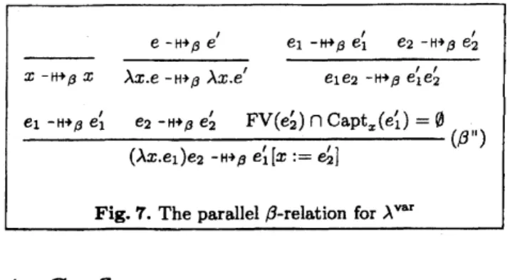
Fresh-Naming As thegeneral$\alpha-/\beta$commutativityre

sultisnot provable,weintroduce thefollowing restricted

a-relation, which only ffesh-names.

$\frac{e_{1}-\mathrm{H}*_{\beta}e_{1}’e_{2}- \mathrm{H}*_{\beta}e_{2}’\mathrm{F}\mathrm{V}(e_{2}’)\cap \mathrm{C}\mathrm{a}\mathrm{p}\mathrm{t}_{x}(e_{1}’)=\emptyset}{(\lambda x.e_{1})e_{2}-\mathrm{H}’\rho e_{1}[x.=e_{2}’]},.(\beta^{1\mathfrak{l}})$

Fig.7. The parallel$\beta$relation for$\lambda^{\mathrm{m}\mathrm{r}}$

4Confluence

The previoussectionestablishesarather large fragment

of the $\lambda^{\mathrm{v}\mathrm{a}\mathrm{r}}$-calculus as susceptible to primitive

equa-tional reasoning. This section summarises and elabo

rates

on

our formally verified efforts to bring this to

bearingon$\beta$-confluence[25].We also presentproofsthat

applythe methodology toprove $\eta-$ and$\beta\eta$ Confluence

4.1 $\beta$ Confluence

The $–*\rho$-relation does not enjoy the diamond

proP-erty because aredex that is contracted inonedirection

of adivergence

can

be duplicated (and erased) in the

other direction by thesubstitutionoperator. Asshown

byTait andMartin-L\"of, thepotential divergence

“blow-uP”

does not materialise because it

can

be controlled by

parallelreduction. Please referto Figure 7for the$\lambda^{\mathrm{v}\mathrm{a}\mathrm{r}_{-}}$

versionof thisrelation.

Lernrna 24 _(BCF) $\cdot-\mathrm{f}1arrow$

.

1 $\beta\acute{\sigma}$ $\pm$ $=$ $\beta\downarrow$

.

}

$|_{\check{\beta}^{\mathrm{O}}}^{;\beta}$

Proof Rather thanprovethis property by an

exhaus-tive case-splitting, thus resulting in aminimally resolv-ing end-term, Ihkahashi observed that the considered

di amond

can

be diagonalised by the relation that

con-tracts all redexes in one step, i.e., by amaimally

re-solving end-term [23]. As we saw in Section 3this is

within reach of thestructuralproofprinciples of$\lambda^{\mathrm{v}\mathrm{a}\mathrm{r}}$

.

$\square$

Definition 26

e$-*_{\alpha 0}e’\Leftrightarrow^{\mathrm{d}\mathrm{e}\mathrm{f}}3\mathrm{z}.\mathrm{e}--\star:\alpha e’z\Lambda z\not\in \mathrm{F}\mathrm{V}(e)\mathrm{U}\mathrm{B}\mathrm{V}(\mathrm{e})$

Thefresh-naming$\alpha$-relation

can

straightforwardly be

proven to commute with the parallel (actually, any)

$\beta$-relation with the proviso that the resolving $\alpha$-steps

are

notnecessarilyfresh-naming(because of$\beta$-incurred

termduplication). Lemma 27 $.-\mathrm{H}arrow$

.

1 $\beta$; $\alpha_{0}\downarrow$ $\mathfrak{g}_{\mathrm{C}}$ $.\vee$ $\}\{*\beta^{\mathrm{o}}$

Similarly, the ffesh-naming $\alpha$-relation canbe shown

toresolve $\alpha$-equivalence toaBCF(althoughtheformal

proofof this is surprisinglyinvolved, cf. [25]$)$.

Lemma 28

$.========\backslash /\backslash \alpha,\cdot$

$\alpha_{00}\backslash _{\mathrm{t}\backslash }$

.

$\alpha_{0}$ (BCF)

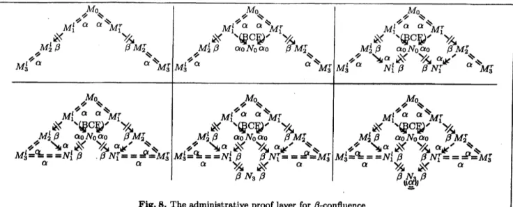
Applying Administration With these results in

place, we canlift Lemma 24 to the real A-calculus.

Lemma 29 $\mathrm{o}(\dashv[]_{\beta})$ A $\mathrm{o}(--*_{\alpha};-\mathrm{H}’\rho)$

Proof As forthe left-most conjunct,see

Figure

8for

the step by step resolution of the definitionally-given

syntactic divergence. We trust the stepsareself-evident

and that it can be seen that aslight adaptation of the

figure also proves the right-most conjunct. $\square$

We are

now

in apositionto establish$\beta$-confluence.

Theorem 30

The Full Proof Burden Areal version ofthe parallel

$\beta$-relation

on

syntax

can

be defined along the lines of

Definition 17(which,further to Lemma 21, turnsoutto

be the real realparallel$\beta$relation.

Definition 25 $\lfloor e_{1}\rfloor-[] f*_{\beta}\lfloor e_{2}\rfloor\Leftrightarrow^{def}e_{1}=_{-j-\mathrm{H}*_{\beta};-=_{\alpha}}^{-_{\alpha}}-$

e2

In order toprovethediamond property for $\dashv\mapsto\beta$,

we

need some

measure

of commutativity between $\alpha-$ and

Confl$(arrow\beta)$ AConfl$($–,$\alpha\beta)$

$\Lambda \mathrm{C}\mathrm{o}\mathrm{n}\mathrm{f}1(--,\alpha \mathrm{c}_{\mathrm{u}}\beta \mathrm{c}_{\mathrm{u}})$

$\Lambda \mathrm{C}\mathrm{o}\mathrm{n}\mathrm{f}1(arrow_{\beta^{\mathrm{H}1}})$

Proof The two topmost conjuncts areequivalent by

Lemma 18. They can alsobe proved independently by

applying the Diamond Tiling Lemma of Appendix $\mathrm{C}$

to the corresponding conjunct in Lemma 29. Thethird

conjunct follows by Lemmas 15 and 16. The final

con-junct follows in

an

analogous

manner.

$\square$

$\prime J\backslash \Lambda f_{0_{\backslash }}$

$\prime\prime\prime^{\prime\backslash }M0_{\backslash }$ $\prime\prime\backslash M0_{\backslash }$

$\grave{\ltimes}<M_{1}^{\iota’\alpha}$

’

$\alpha\grave{\grave{M}}_{1}^{r}\grave{/}_{4}$

$\aleph^{\backslash }<M_{1}^{\iota\alpha\alpha},M_{1}^{r}\backslash \mathrm{g}\mathrm{c}\mathrm{p}\grave{/}\mathrm{g}$

$\grave{\ltimes}<\backslash \not\in^{\mathrm{c}\mathrm{p}’\grave{/}_{4}}M_{1}^{\iota^{J\prime}\alpha\alpha}M_{1}^{r}$

$M_{2}^{\iota}\beta$

$\beta M_{2}^{r}\backslash \backslash$ $\prime\prime M_{2}^{l}\beta$ $\alpha \mathrm{o}N_{0}\alpha_{0}$

$\beta \mathrm{A}f_{2}^{r}\backslash \backslash$

$M_{2}^{l}\beta$ $\alpha 0N_{0}\alpha_{0}$

$\beta,M_{2}^{r}\backslash \backslash$

$M_{3}^{\iota’\alpha}\acute{\prime\prime}$

$\alpha\grave{\grave{M}}_{3}^{\mathrm{r}}M_{3}^{\iota^{J}\alpha}$’ $\alpha\grave{\grave{M}}_{3}^{r}M_{3}^{\iota^{J}\acute{\alpha}}\prime\prime$ $[searrow]\alpha \mathrm{A}^{\backslash ’}N_{1}^{l}\beta$ $/\mathrm{g}\alpha_{*}\beta N_{1}^{r}$

$\alpha\grave{\grave{M}}_{3}^{r}$

$M_{0}$ $M_{0}$ $M_{0}$

,/ $\backslash \backslash$

$\mathrm{a}^{\backslash }<\backslash \mathrm{g}\mathrm{c}\mathrm{p}’)’M_{1}^{\iota’\alpha\alpha}M_{1}^{r}\prime 4$ $\mathrm{k}^{\backslash }\cross^{M_{1}^{\iota^{J}\acute{\alpha}\grave{\alpha}}M_{1}^{r}}\prime \mathrm{G}^{\mathrm{c}}\Psi’\grave{/}\mathrm{g}’\backslash$ $\mathrm{k}^{\backslash }\cross’ \mathrm{g}\mathrm{c}\mathrm{p}’\cross_{4}M_{1}^{\iota\alpha\grave{\alpha}}M_{1}^{r}\prime\prime^{\prime\backslash }$

$[searrow]\alpha\aleph^{\cross}$ $\grave{/}4\alpha_{\mu}$ $[searrow]\alpha \mathrm{A}^{}$ $\grave{/}_{4}\alpha_{C}$ ” $[searrow]\alpha\aleph^{\cross}$ $\grave{/}4\alpha_{\mathrm{g}}$ $\prime\prime M_{2}^{\iota}\beta$ $\alpha 0N_{0}\alpha 0$

$\beta,M_{2}^{r}\backslash \backslash$ $’,M_{2}^{l}\beta$ $\alpha_{0}N_{0}\alpha_{0}$ $\beta,M_{2}^{f}\backslash \backslash$

”

$M_{2}^{l}\beta$ $\alpha \mathit{0}N_{0}\alpha_{0}$

$\beta,M_{2}^{r}\backslash \backslash$

$M_{\mathrm{s}_{\alpha}^{===N_{1}^{\mathrm{t}}}}^{l^{J_{J}}\underline{\not\subset}}\beta$ $\beta N_{1}^{r}==^{\underline{B}}\grave{\grave{=}}M_{3}’\alpha M\mathrm{s}_{\alpha}^{l^{J}\underline{\mathrm{L}}}===N_{1}^{l}’\beta$ $\beta N_{1}^{r}==^{\underline{\mathrm{p}}}\grave{=}\grave{M}_{3}^{r}\alpha M_{\mathrm{a}_{\alpha}^{===N_{1}^{\iota}}}^{l\underline{\not\subset}}\beta$ $\beta N_{1}^{r}==_{\alpha}^{\underline{\mathrm{p}}}\grave{=}\grave{M}_{3}^{r}$

$\mathrm{y}_{A}$

\‘A<

_$)’A$

\‘A<

$\beta N_{\theta}$

I

$\beta_{\iota_{\vee}^{N\beta}}\iota_{-}d/$

Fig.8. Theadministrativeproof layerfor$\beta$-confluence

$M_{0}$

” $\backslash \backslash$ $\prime\prime J\alpha$

’

$\alpha^{\backslash }\backslash \backslash \backslash$

$M_{1}^{l}$ $M_{1}^{r}$

$\mathrm{A}\Upsilon_{2}^{\iota^{-_{\eta}’}}$

’

$\backslash \alpha_{0N_{0}}^{*\iota_{\alpha_{0}}^{\prime’}}\backslash$ $\backslash \eta_{M_{2}^{r}}^{\mathrm{Y}}\backslash$

$\prime^{\prime’}J\alpha J’$ $\backslash [searrow]\alpha.$”

$\backslash ’\backslash \backslash \eta\tilde{N}_{1}^{r}=====\grave{=}M_{3}^{r}\alpha\backslash *’\alpha^{\backslash }\backslash \backslash$

$M_{3}^{l}=====N_{1}^{1}\alpha\eta$

$\alpha$ $\backslash \mathrm{t}$ $t’$

$\eta\eta\prime\prime^{N_{\theta}}\backslash \backslash$

$\backslash \backslash ^{\alpha_{J/}}\sim\vee$

$M_{1}^{\iota_{==M_{0}==M_{1}^{r}}^{\alpha\alpha}}$

$M_{2}^{l}==N_{1}^{\iota^{-}\eta}\eta_{\vee’’}’$ $\backslash \backslash \grave{\eta}_{N_{1}^{r}=}^{\mathrm{Y}}\cong_{M_{2}^{r}}\backslash \eta$

” $\alpha$

$\backslash [searrow]$ $0^{\prime’}$

$\prime\prime\prime$’

$\alpha$ $\alpha$ $\backslash \backslash$

$\backslash \backslash$

$M_{3}^{l}$

$\eta\eta/F^{2}\backslash \backslash ^{\underline{\alpha}_{J/}}rightarrow\backslash \backslash$

$M_{3}^{r}$ $\alpha\backslash \backslash$

Fig. 9. The administrativeproof layerfory7Confluence

4.2 $\eta$-Confluence

Unlikethe$\beta$-relation, $\eta-$-reduction is natively

renaming-free:

Lemma 31 ($\alpha/\eta$ Commutativity)

$\mathrm{I}\mathrm{I}.\vec{\eta}--$

:

ai

.

$\vee 1\alpha$

$\sim.,’\grave{\eta}^{\mathrm{b}\circ}$

Lemma 32 ($\eta$ Commutativity)

$\eta\downarrow.l^{\eta}\mathrm{i}_{1}^{--}\vec{\eta}_{\mathrm{f}}\vee\backslash \cdot \mathrm{O}^{\cdot}$ $\wedge$

$\eta i$

.

$\vec{\eta}\backslash \mathrm{f}.\eta$

Proof The left-most conjunct $\mathrm{i}\mathrm{s}\mathrm{s}\mathrm{t}\mathrm{r}\mathrm{a}\mathrm{i}\mathrm{g}\mathrm{h}\mathrm{t}\mathrm{f}\mathrm{o}\mathrm{r}\mathrm{w}\mathrm{a}\mathrm{r}\mathrm{d}1\mathrm{y}\grave{\eta}^{;\grave,0}$

provable by structural

means.

The proof of the

right-most propertyfollows from the left-mostasdisplayed in

Figure 9. The top part ofthe figure is aproofby the

general method; the lower part is anoptimisedversion

that takes advantage of$\eta$ commuting with $\alpha$, not just

with $\alpha_{0}$

.

$\square$

Theorem 33 Confl(–*\eta )\wedge Confl(\rightarrow \eta ) $\Lambda$Confl(–*\mbox{\boldmath $\alpha$}\eta )

Proof The twoleft-most conjunctscanbe established

from the corresponding conjunctsin Lemma 32 by the

Hindley-Rosen Lemma of Appendix C. The right-most

conjunct

can

be established either by the Commuting

Confluence Lemma of Appendix $\mathrm{C}$ applied to the

left-most conjunct and generalisations of Lemmas 11 and31

or, alternatively, it can be observed that the two

right-most conjunctsare equivalent byLemma 18. $\square$

4.3 $\beta\eta$-Confluence

Sincethe$\eta$-relation isnatively renaming-freeandthe$\beta-$

relation relies on the a-relation,

we

must show that $\eta-$

commutes with combined $\alpha\beta$-reduction in order to ap

ply the CommutingConfluence Lemma of Appendix C.

Lemma 34

$\mathrm{I}.\vec{\eta}--$

;

$|.\eta_{\dagger}.\mathrm{l}\cdot,\eta_{\mathrm{f}}--*--*\sqrt 1\alpha\beta\Lambda\alpha\beta\star \mathrm{t}^{\mathrm{t}}.\alpha\beta$

$\beta\downarrow \mathrm{I}$

.

,$\acute{\eta}^{\mathrm{o}}.\mathrm{s}^{\xi_{\alpha\beta\wedge\alpha\beta\downarrow}}\mathrm{I}.$

. $*\triangleright\eta^{\mathrm{o}}$

.

,

$\mathrm{m}\acute{.}\mathrm{A}\eta^{\mathrm{O}}$

Proof The proofof theleft-most conjunctis

straight-forward. The $\alpha$-step in the resolution on the right is

needed for the obvious divergence

on

$\lambda z.(\lambda y.e)x$, with

$x\neq y$. Themiddleconjunctcombines the left-most

con

junct and Lemma 31. Theright-most conjunct follows

from the middle by the Hindley-Rosen Lemma of Ap

pendixC. $\square$

$M_{0}$

” $\backslash \backslash$ $\prime’\prime’\alpha$ $\alpha^{\backslash }\backslash \backslash \backslash$

$M_{1}^{l}$ $M_{1}^{r}$

$M_{2}^{l\check{\beta}}$

”

$\backslash \alpha_{0N_{0}}^{*\iota_{\alpha_{0}}^{\prime’}}\backslash$ $\backslash \backslash \eta\tilde{M}_{2}^{r}$

$M_{8}^{l}=====N_{1}^{\mathrm{I}\beta}\alpha\backslash$ $\prime^{\prime’}J’\alpha$

’

$\backslash [searrow]\alpha\vee^{\prime’}$

$\backslash ’\backslash \backslash \eta\tilde{N}_{1}^{\mathrm{r}}======M_{3}^{r}\dot{\alpha}\mathrm{f}’\alpha^{\backslash }\backslash \backslash \alpha\backslash \backslash$

$\eta[searrow]\alpha_{\acute{\alpha}\beta}/F_{\frac{\alpha}{\vee}}^{\mathrm{a}}\backslash \backslash \backslash \backslash //$

$M_{0}$

$\prime_{J}$ $\backslash \backslash$

$\prime_{J}$ $\backslash \backslash$

$M_{1}^{\iota_{====\grave{\grave{=}}M_{1}^{\mathrm{r}}}^{J}}’\alpha\alpha$

$M_{2}^{\check{l}}\beta$

”

$\backslash \alpha\backslash \grave{\eta}_{N_{0}=====\tilde{=}M_{2}^{\mathrm{r}}}^{\mathrm{Y}\grave{\eta}}$

” $\backslash$ $\alpha$ $\backslash \backslash$

$M_{3}^{l^{\prime’}}"\alpha$

$\backslash \eta^{*t_{\alpha\beta}’}\prime F_{\alpha_{J/}}^{1}\backslash \backslash =\backslash \backslash$

$\alpha^{\backslash }\backslash \grave{\grave{M}}_{3}^{r}$

Fig.10. The administrative proof layer for$\beta\eta-$-confl

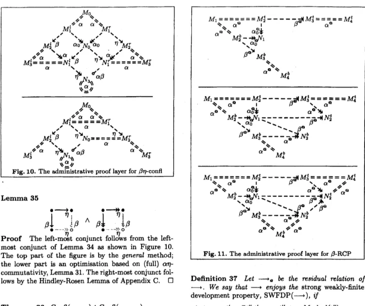
Lemma 35

Proof The

$\beta \mathrm{l}\mathrm{e}\mathrm{f}.\mathrm{t}- \mathrm{m}\mathrm{o}\mathrm{e}\mathrm{t}\mathrm{c}\mathrm{o}\mathrm{n}\mathrm{j}\mathrm{u}\mathrm{n}\mathrm{c}\mathrm{t}.\mathrm{f}\mathrm{o}11\mathrm{o}\mathrm{w}\mathrm{s}\mathrm{f}\mathrm{r}\mathrm{o}\mathrm{m}\mathrm{i}\vec{\eta}\mathrm{i}_{l}$ }

$\acute{\dot{\acute{\grave{\dot{\eta}}}}}^{\grave{\mathrm{o}}}\hat{\dot{\eta}}^{\mathrm{O}}\iota\beta^{\Lambda}\beta \mathrm{i}\vec{\eta}$

}}

$\mathfrak{x}\beta$

the

left-most conjunct of Lemma 34 as shown in Figure 10.

The top part of the figure is by the general method;

the lower part is an optimisation based

on

(full)

otq-commutativity, Lemma31. The right-most conjunct

fol-lows bythe Hindley-Rosen Lemma of Appendix C. $\square$

Theorem 36 Confl$(arrow\beta\eta)\Lambda \mathrm{C}\mathrm{o}\mathrm{n}\mathrm{f}1(--*_{\alpha\beta\eta})$

Proof We first observe that the two conjuncts

are

equivalent by Lemma 18. They

can

also be proved

in-dependently by the Commuting Confluence Lemma of

Appendix $\mathrm{C}$ applied toTheorems 30 and 33 aswell as

Lemma 35 andLemma 34, respectively. $\square$

5Residual

/3-COnfluence

Wesaythatthereflexive,transitive closure of aresidual

relation is the associated developmentrelation, astepof

which issaidto be complete if the target term does not

contain amark,unMarked(-).With this terminology in

place,

we

defineaweakened version of the strong finite

development property.8

6 _{The strong finite development property alsorequiresthat}

theresidual relation is stronglynormalising.Itistypically

usedto prove (residual)confluence.

Definition37 $Letarrow\Phi$ be the residual relation

of

$arrow$. We say $thatarrow enjoys$ the strong weakly-finite

development property, SWFDP$(arrow)$,

if

1. $tarrow_{q}t’\Rightarrow\exists t’.t^{\prime-\epsilon}t’$A $\mathrm{u}\mathrm{n}\mathrm{M}\mathrm{a}\mathrm{r}\mathrm{k}\mathrm{e}\mathrm{d}(t’)$

-developments can be completed

2. $tarrow_{o}t_{i}\wedge \mathrm{u}\mathrm{n}\mathrm{M}\mathrm{a}\mathrm{r}\mathrm{k}\mathrm{e}\mathrm{d}(t_{i})\Lambda i\in\{1,2\}\Rightarrow t_{1}=t_{2}$

-completions

are

unique

To motivate the name of the proPerty, we see that, indeed:

Proposition a8 SWFDP$(arrow)\Rightarrow \mathrm{W}\mathrm{N}(arrow_{\mathrm{p}})^{7}$

Proof By Definition 37 1. and reflexivity of$arrow 0$.$\square$

Surprisingly, perhaps,

we

have that already theSWFDP

implies residual confluence.

Lemma 39 SWFDP$(arrow)\Rightarrow \mathrm{C}\mathrm{o}\mathrm{n}\mathrm{f}1(arrow_{\mathrm{n}})$

Proof Consider the following divergence:

$M_{1}M_{2}\mathrm{B}\swarrow^{M}[searrow]@$

7_Thepredicate$\mathrm{W}\mathrm{N}(-)$stands forWeak Normalisationand

meansthat all terms reduce to anormal form

By Definition 37, 1., there exist $N_{1}$, $N_{2}$, such that

$\mathrm{u}\mathrm{n}\mathrm{M}\mathrm{a}\mathrm{r}\mathrm{k}\mathrm{e}\mathrm{d}(N_{1})$, $\mathrm{u}\mathrm{n}\mathrm{M}\mathrm{a}\mathrm{r}\mathrm{k}\mathrm{e}\mathrm{d}(N_{2})$ and:

$@\swarrow^{M}[searrow] \mathrm{n}$

$M_{1}$ $M_{2}$

@\downarrow

$\downarrow@$

$N_{1}$ $N_{2}$

By transitivity of $arrow@$ and Definition 37, 2., we

see

that, in fact, $N_{1}=N_{2}$ and we

are

done. $\square$

With direct reference to Section 3, we define the

following property, which is fairly easily proven to be

equivalent to the SWFDP.

Definition 40 A relation, $arrow$, enjoys the

residual-completion property, RCP$(arrow)$,

if

there exists $a$

residual-completion relation, “$a$

’such

that:

1. $-_{\emptyset}\subseteqarrow a$ -residual-completion is a development 2. -$\cdot$ $\overline{residu}^{\Phi}al- c\mathrm{q}mpletioni\mathrm{o}(\mathrm{N}\mathrm{F}_{u})$ totally completes 3. $\cdot$ $\backslash _{\varpi}.\infty$ $\prime\prime f$

.

-residual-completion is residually

_cO-final

Lemma 41 RCP(\rightarrow )\Leftrightarrow SWFDP(\rightarrow )

Our interest intheRCP is its constructive nature, in

particular when the residual-completion relation is de

fined as acomputablefunction the way we didin

Sec-than3.

Lemma42 RCP(\rightarrow \beta ) $\Lambda$ SWFDP(\rightarrow \beta )

Proof Weprovetheleft-most conjunct. Clause 1.

fol-lowsfromtheeasilyestablishedfactthat$–\triangleleft_{\beta^{\Phi}}\subseteq--,\beta@$

.

Clause 2follows from Lemmas 21 and 28. Finally,

Clause3isproved

_as

shown inFigure 11. $\square$

Theorem 43 Confl(\rightarrow \beta u)$\Lambda \mathrm{C}\mathrm{o}\mathrm{n}\mathrm{f}1(--*_{\alpha^{\mathrm{g}}\beta^{\mathrm{g}}})$

We see that $\mathrm{S}\mathrm{N}(\sim\beta^{\mathrm{Q}})$ (i.e., the difference between

the SWFDP and the strong finite development prop

erty) is not needed for concluding confluence bom a

residual analysis of the $\beta$-relation, something which

is in stark contrast to established opinion [2, p.283].

Strong finite development essentially implies confluence

through Newman’sLemma,thus relyingcruciallyon the

(non-equational) $\mathrm{S}\mathrm{N}$-propertyfor the residual relation.

We think it anice “purification” of the equational

im-port ofresidualtheory that

an

externallyjustified

termi-nation property is not needed for concluding confluence.

6

$\eta-\mathrm{o}\mathrm{v}\mathrm{e}\mathrm{r}-\beta$

-POstpOnement

As wellas condensing Tait and Martin-Ldf$\mathrm{s}$useof

par-allel $\beta$-reduction for proving $\beta$-confluence, Takahashi

[23] also shows how to adapt the parallel-reduction

technology to other typical situations in the equational

theory of the A-calculus. Onesuch situation is for

prov-ing $\eta- \mathrm{o}\mathrm{v}\mathrm{e}\mathrm{r}-\beta$-postponement, cf. Figure 12. The proof

presented by Takahashi [23] essentially goes through

up toBCF-initiality as itstands, albeit not completely.

Rather than focusingonthelow-level technicaldetails,

this section merely shows the Administrative and Ab

stract proof layers of our formalisation ofTakahashi’s

proof.

Thenotion of commutativity thatwehave considered

so

far is orthogonal innature to thatemployed in the$\eta-$

$\mathrm{o}\mathrm{v}\mathrm{e}\mathrm{r}-\beta$-Postponement Theorem. Whereas the former

can

be described as divergence commutativity, this section

focuseson composition commutativity.

Lemma 44 (BCF) $\{|>\beta$ $\circ$ 1 ; $\eta_{\star}^{\mathrm{B}}$ $\Leftarrow\dot{*}\eta$ $.-\mathrm{H}_{\vec{\beta}}$

.

39

Proof The parallel$\eta$-relationisused to allow for the duplication ofa$\eta$-redex by the$\beta$-contractionwhen the

latter is performed first. The parallel$\beta$-relation,onthe

otherhand, isused, _{e.g., for}thefollowing situation:

$\underline{\mathrm{C}\mathrm{a}\mathrm{p}\mathrm{t}_{x}}(e_{1})\cap \mathrm{F}\mathrm{V}(e_{2})=\emptyset$ $/a^{\mathrm{w}\mathrm{h}})\underline{e_{1}}-*_{\beta^{\mathrm{w}\mathrm{h}}}e_{1-\prime\cap \mathrm{n}^{\mathrm{W}\mathrm{h}_{1}}}’$

$\overline{(\lambda x.e_{1})e_{2}}--*_{\beta^{\mathrm{w}\mathrm{h}}}e_{1}[x\cdot.=e_{2}]$ $\backslash \mu$

$J\overline{e_{1}e_{2}}--*_{\beta^{\mathrm{w}\mathrm{h}}}e_{1}’e_{2}$

$\backslash arrow \mathrm{w}$ /

Fig. 14. Weak-head$\beta$-reduction

$(\lambda x.(\lambda y.e_{1})x)e_{2\eta}-,(\lambda y.e_{1})e_{2\beta}--*e_{1}[y:=e_{2}]$

This reduction sequencecommutes into aleading

par-allel $\beta$-step with atrailing$\eta$-step, which is inthis

case

is reflexive:

$(\lambda x.(\lambda y.e_{1})x)e_{2\beta}-\mathrm{H}*\mathrm{e}\mathrm{i}[\mathrm{y}:=x][x:=e_{2}]$

BCF-initiality is used to enable the double ($\mathrm{n}$-fold, in

general) substitution in the commuted reduction

se-quence. $\square$

$\frac{e_{1}}{e_{1}\mathrm{e}_{2}}--\_{\beta^{1}}--*_{\beta^{1}}e_{1}’ e_{2}e_{1}’$$(@_{1}^{1}) \frac{e_{2}-*\rho}{e_{1}e_{2\beta^{1}}-}*e_{2}’e_{1}e_{2}’$ $(@_{2}^{\mathrm{I}})$

$\underline{e-*_{\beta}}e’$

$/1^{1}1$

$-\overline{\lambda x.e--*_{\beta^{1}}}\lambda x.e’\iota-r$

–

$-/1\Gamma--^{1}\backslash \underline{e_{1}}-\mathrm{H}’\beta \mathrm{I}e_{1}’$$e_{2}-\mathrm{H}’\beta e_{2}’$ $/\cap \mathrm{n}^{\mathrm{I}}\backslash$ $\overline{z}-\mathrm{H}*_{\beta^{\mathrm{I}x}}$ $1$ $\mathrm{v}a\iota_{1\mathfrak{l}/}\overline{e_{1}e_{2}}\sim \mathrm{H}’\beta’e_{1}’e_{2}’$ $\backslash \infty_{\mathrm{I}\mathrm{I}}/$ $\underline{e-\mathrm{H}*_{\beta}}e’$ /11

$\overline{\lambda z.e-\mathrm{H}\mathrm{r}_{\beta^{1}}}\lambda x.e’$

$\backslash -|\dagger J$

Fig. 15. Innerandparallel inner$\beta$-reduction

Lemma 45

.

_}

$\dagger^{\beta}\sim$

$0$

$\eta\neq$ $\mp_{\dot{\nu}\eta}^{\mathrm{I}}$

$.\dashv\vdash$

.

Proof Please refer to Figure 13 for the details of the

proof. Anovel aspect of the proof is the existence ofan

$\alpha_{0}$-step from$M_{5}$ to $N_{2}$

.

By construction,

we

knowthat

the two terms

are

a-equivalent. Asimple lemma shows

that $N_{2}$ isaBCF because$\eta-$-reduction preserves BCFs.

The final result that is needed, i.e., that $\alpha_{0}$ reduction

can reach any BCF that is $\alpha$-equivalent to the start

term,

can

also be provedby structural

means

but it is notas straightforward as couldbeimagined. This is due

to theneed for the target BCFto be any BCF. Cl

Withthe onenecessarytechnical lemmain place, we

present the postponement theorem. Theorem 46

$.,-\backslash _{\mathrm{Y}}\backslash _{\mu},$

, $.-\mathrm{O}$

$\beta\eta’\acute{\tilde{\eta}}^{\nabla}"$

.

Proof By reflexive, transitive induction in $arrow\beta\eta$.

The only interesting case is the transitive case, which

follows in amanner akin totheHindley-RosenLemma

ofAppendix$\mathrm{C}$ using Lemma 45. $\square$

7

$\beta$

Standardisation

Standardisation is also acomposition-commutativity result like postponement. It is avery powerful result

that, informally speaking, says that any reduction

se-quence

can

be performed left-to right. Standardisation

implies results such

as

the left-most reduction lemma,

etc., [2], and guarantees the existence of

evaluation-orderindependent semantics [20].

This section addresses three different approaches to

proving standardisation due to Mitschke [18], Plotkin

[20], and David [5], respectively. The three approaches

are fairy closely related, with Plotkin’s proof bridging

the other two, so to speak. Mitschke’s and Plotkin’s

proofs bothusesemi-standardisation while David’s and

Plotkin’s bothcanbe described

as

absorption

standardi-sation. In spite (actually because) ofthis, onlyPlotkin’s

approach is formally provable by the proof principles we areconsidering. Weshall examine the failures of the

other twoproofs closely.

7.1 Semi-Standardisation with Hereditary

Recursion

In this section, we shall pursue aslight adaptation of

Takahashi’s adaptation [23] ofMitschke’s proof [18].

In-stead ofheadand acorresponding notion of inner

reduc-tion, we base the proofon weak-head reduction. This

does not affect the formal status oftheprooftechnique

but does allow us to reuse the results of this section

when pursuing Plotkin’s approach. The main proof

bur-den is to show that(weak-)headredexes cancontracted

before any inner redexes,s0-calledsemi-standardisation.

Definition 47 Weak-head$\beta$ reduction, –

$,\beta^{\mathrm{w}1}‘$

,

is

de-fined

in Figure

_14.

The corresponding (strong) inner,

$–\#_{\beta^{1}}$, andparallelinner, $-\mathrm{H}*_{\beta^{\mathrm{I}}}$,

$\beta$-relations

are

defined

in Figure 14.

introduce an$\alpha_{1}$-relationthatcorresponds to the wBCF-predicate. The $\alpha_{1}$-relation isless well-behaved than the $\alpha_{0}$-relation butwe can,at least, show that itcommutes

with $-+\beta$ (and thus $-*_{\beta^{\mathrm{w}\mathrm{h}}}$), up to a-resolution. The

left-most conjunct of the lemma, follows by rule

induc-thanin $-\mathrm{H}’\beta^{\mathrm{I}}$

.

$[]$

At this point, the idea is to recursive over the $\circ$ in

Lemma 50 and show that the sub terms in which the

outgoing $arrow\beta^{1}$-step

are

ordinary $\beta$-steps, themselves

canbe semi-standardised andso on. Unfortunately, the

$\circ$ is quantified

over

a-equivalence classes, for which

no

recursion is possible and

we

arestuck.

Lemma 48

$\beta_{i}^{\mathrm{w}\mathrm{h}}\circ\ell_{\mathrm{w}}^{\beta^{1}}$ (BCF).’-$-\dashv\vdash-\vec{\beta}$

.

$\Lambda$

Proof Please refer to Figure 16 for the proofofthe

right-most conjunct based on the left-most conjunct,

wich, in turn, isproved by rule induction$\mathrm{i}\mathrm{n}-\mathrm{H}\_{\beta}$

.

[:]

The use of BCF-initiality in the left-most conjunct

above guarantees that weak-head redexes can be

con-tracted without waiting for the contraction of

an

inner

redex to eliminate avariable clash.

Lemma 49

(BCF)

$\cdot\backslash \nu_{\mathrm{p}.’\beta^{\mathrm{w}\mathrm{h}}}\beta|\}\beta,\dot{\lambda}\acute,$

.

$\Lambda$

$\lambda_{\beta^{1}}../_{\beta^{\mathrm{w}\mathrm{h}}}^{\lambda^{\mathrm{h}}}|\}^{\beta}$

.

Proof Please refer to Figure 17 for the proof of the

right-most conjunct based on the left-most. We first

note that the figure invokes the obvious adaptation of

Lemma 27 to $-\mathrm{H}*_{\beta^{1}}$

.

Although the proofas awhole is

similartothat of$\eta- \mathrm{o}\mathrm{v}\mathrm{e}\mathrm{r}-\beta$-postponement, cf.Lemma 45,

wedo not have that$-\mathrm{H}\star_{\beta}1$ preservesBCFs,asis the

case

with $-\mathrm{H}\star_{\eta}$. Instead,we canintroduce aweakened notion

of BCF, wBCF, that allows identical binders to

occur

in adjacent positions (but not nested and not

coincid-ing with any bee variables) and show that $-\mathrm{H}’\beta^{1}$ sends

BCFstowBCFs. In the

same

manner

that$\alpha_{0}$-reduction

and the BCF-predicate correspond to each other,wecan

7.2 Hereditary Weak-Head Standardisation

Plotkin [20] defines standardisation

as

the least

contextually-closed relation on terms that enjoys

left-absorptivity over weak-head reduction. The following

presentationoftheproofmethodologyowesagreatdebt

to McKinna and Pollack [17]. The difference between

their and our presentation is that we focus on

prov-ability with structuralinduction, etc., while they work

with analternativesyntactic framework that is derived

from first-0rder abstract syntax with $\mathrm{t}\mathrm{f}\mathrm{u}/0$-sorted

vari-ablenames.The proof requirements in their setting and

in

ours are

substantially different asaresult.

A First (Failing)Approach Afirst approach, which

im-mediately fails, is todefinePlotkin’s relation directlyon terms.

e $-,\beta^{\mathrm{w}\mathrm{h}e’}e’\succ-\dashv_{\mathrm{P}}e’$

e $\succ-\mathrm{r}_{\mathrm{P}}e’$ x

$\succ-\tau_{\mathrm{P}}x$

$\underline{e_{1}\succ-\dashv \mathrm{p}e_{1}’e_{2}\succ-\dashv \mathrm{p}e_{2}’}\underline{e\succ-\dashv \mathrm{p}e’}$

$e_{1}e_{2}\succ-\dashv \mathrm{p}e_{1}’e_{2}’$ $Xx.e\succ-\dashv \mathrm{p}\lambda x.e’$

As standardisationpertains to all $\beta$-reductions(i.e., $arrow\beta$, not just $-\cdot\beta$), the naive approach needs the

full A-calculusto be renaming-free,which it isnot. The

problemmanifests itselfinthe required administrative

prooflayer for thestandardisationpropertyand its

ex-act nature isof independent interest. Thepoint is that,

even

if it is possible to prove the following key property

(which,in fact,

seems

tobe the$\mathrm{c}\mathrm{a}\mathrm{s}\mathrm{e}^{8}$

),

we

cannot prove

8_{Coincidentally, it is interestingto notethat theproofof}

the property canonly be conductedby ruleinduction in

$\succ-\dashv \mathrm{p}$ andnot $\mathrm{i}\mathrm{n}-*\rho$.

$M_{1}$ $M_{1}$

Il $\backslash$

11 $\backslash$ $\alpha$1l

$\backslash \backslash$

$\alpha 0$ $\alpha$$||$ $\backslash$ $\mathrm{o}0$

41 $*$ (BCF) ₁₁ $[searrow]$ (BCF)

$M_{2}-\ovalbox{\tt\small REJECT}_{0_{\mathrm{I}\star}}^{N_{1}}|$ $M_{2}-\theta_{0}^{N_{\iota_{\star}}}\mathrm{I}$ ’

1 1 $\backslash$ 1

$\beta\downarrow|$ $\backslash \backslash$ $\beta\downarrow$ $\beta\downarrow(\mathrm{w}\mathrm{B}\mathrm{C}\mathrm{F})$ $\beta\downarrow$

$\alpha 1\mathrm{I}M_{3}-1\mathrm{I}k^{N_{2}}$ $\backslash \mathrm{t}1$ $\alpha||\mathrm{I}M_{3}-\mathrm{t}_{\mathrm{I}}^{N_{2}^{a}}\mathrm{l}|$ $\backslash$ $/$ I 1l _’$\alpha_{1}|$ 1 11 1 ’ $M_{4}\mathrm{I}|//$ 1 $\mathrm{g}_{\mathrm{I}}|$ $M_{4}|\mathrm{I}$ $\mathrm{I}\mathrm{I}$ $\mathrm{g}_{\mathrm{I}}/$ $\alpha \mathrm{I}|/$ $\dot{\mathrm{f}}1$ / $\alpha||$ $M_{6}^{\mathrm{I}\mathrm{I}J}\mathrm{Y}$ $\mathrm{i}1$ $\mathit{1}$

$M_{5}^{\mathrm{I}\mathrm{I}}-\ovalbox{\tt\small REJECT}_{0}^{N_{2/}^{b}}\mathrm{Y}\gamma/\alpha 0\downarrow_{(\mathrm{B}}\phi)$

$\mathrm{P}^{\mathrm{I}}$ ’ $\mathrm{p}[perp]^{\mathrm{I}}$ $[perp]\langle \mathrm{p}$ $\mathrm{p}[perp]^{1}$ $\mathrm{P}[perp]^{J}\vee \mathrm{p}$ $M_{6}-\not\supset^{N_{3}}1\mathrm{I}$ $M_{6}-?^{N_{3}}\mathrm{I}1$ $\alpha$$11$ _” $\alpha$ $||$ ’ 11 $\iota_{\alpha}$ 11 $g_{\alpha}$ $M\tau$ $M_{7}$

$\lambda y.e_{1}=_{\alpha\alpha \mathrm{w}\mathrm{h}}==\lambda y’.\mathrm{e}_{1}’-+\tau\backslash \mathrm{I}\beta \mathrm{I},r_{\alpha}\backslash \backslash |\mathrm{I}\lambda y^{l}.e_{2}’===\lambda z.e_{2}\succ-\dashv\lambda x.e_{3}$

$\backslash \backslash \mathrm{u}\downarrow^{\alpha 0}$ $\beta^{\mathrm{I}}$

$\downarrow^{\alpha}$

,

’

’

$\alpha_{\lambda x.e_{0}--|\vdasharrow\lambda x.e_{0}’}$

Fig.19.The administrative prooflayerforthe$(\lambda_{\succ\tau_{\mathrm{w}\mathrm{h}}})$ case ofLemma 54

Combining Term Structure and $a$-Collapsed Reduction

In order to avoid these problems, we adapt the above

definition slightly. Definition 52

$\frac{\lfloor e\rfloorarrow_{\beta^{\mathrm{w}\mathrm{h}}}\lfloor e’\rfloor e’\succ-\dashv_{\mathrm{w}\mathrm{h}}e’}{e\succ-\dashv_{\mathrm{w}\mathrm{h}}e’}(\mathrm{w}\mathrm{h}_{\mathrm{p}\mathrm{r}\mathrm{e}})$

$\overline{x\succ-\dashv_{\mathrm{w}\mathrm{h}}x}(\mathrm{V}_{\succ \mathrm{t}_{\mathrm{w}\mathrm{h}}})$

Fig.18. Failed administrative proof layer for

left-absorptivityof progression standardisation

full standardisation but at most standardisationof the

renaming-ffeefragment ofthe $\lambda^{\mathrm{v}\mathrm{a}\mathrm{r}}$-calculus.

(BCF)$.\prime \mathrm{f}_{\backslash t\backslash }-\sim^{\beta}.\mathrm{v}\cdot-\gamma_{\mu}^{\mathrm{P}}$

.

$\mathrm{P}$

Please refer to Figure 18 for the only two sensible

approachestothe administrative proof layer for the

fol-lowing property, which is derived from the one above.

Non-Lemma 51

$.\mathrm{A}_{\backslash \backslash _{\backslash }\wedge}-_{\mathrm{r}\wedge*}^{\beta},\cdot-\gamma^{\grave{\mathrm{P}}}\prime\prime\prime\acute{\mathrm{p}}$

.

$\frac{e_{1}\succ-\tau_{\mathrm{w}\mathrm{h}}e_{1}’e_{2}\succ-\dashv_{\mathrm{w}\mathrm{h}}e_{2}’}{e_{1}e_{2}\succ-\dashv_{\mathrm{w}\mathrm{h}}e_{1}’e_{2}},(@\succ \mathrm{t}_{\mathrm{w}\mathrm{h}})$ $\frac{e\succ-\tau_{\mathrm{w}\mathrm{h}}e’}{\lambda x.e\succ-\tau_{\mathrm{w}\mathrm{h}}\lambda z.e’}(\lambda_{\succ\tau_{\mathrm{w}\mathrm{h}}})$

The definition mixes the advantages of being able to

define relations inductively

over

terms with the

use

of

reduction in the real A-calculustoavoid issues of

renam-ing. Note, however, that, further to the failed proof of

Lemma 4, it is by no meansobvious whether this

mix-turn $\mathrm{w}\mathrm{i}\mathrm{h}$ lend itself to primitive structural reasoning.

Theproof-technicalissuesurfacesin the $(\mathrm{V}_{\succ 1})\mathrm{w}11$

case

of

theproofof Lemma 54. Lemma 53

$\beta\neq$

.

$\beta^{\mathrm{w}\mathrm{h}}\iota^{\backslash }\sim 0_{\mathrm{f}}=_{\beta^{1}}^{l}.’$

.

$.arrow$

.

Proof The propertycan$\theta_{\mathrm{e}}^{\mathrm{w}}h\mathrm{e}\mathrm{r}\mathrm{i}\mathrm{v}\mathrm{e}\mathrm{d}$

fromLemmas48

and 49 based on asuitable adaptation of the

Hindley-RosenLemma, cf. AppendixC. $\square$

The left-most diagram in the figure attempts to align

itself with Figure 13, which fails because $\succ-\dashv \mathrm{p}$ only

commutes with $–\star_{\alpha_{0}}$

.

The right-most diagramadheres

to this and fails because of the inserted $–\mathrm{r}_{\alpha 0}$, which

we cannot incorporate into the syntactic version of the

property. It iseven straightforward to

come

upwith a

counter-example.

(Xs.ss)(Xx.Xy.xy) $–*\beta(\lambda x.\lambda y.xy)(\lambda x.\lambda y.xy)$

We

can

turn the end-term into

an

$\alpha$-equivalentBCF

as

it happens, which standardises:

$(\lambda x_{1}.\lambda y_{1}.x_{1}y_{1})(\lambda x_{2}.\lambda y_{2}.x_{2}y_{2})\succ-\dashv \mathrm{p}\lambda y_{1}.\lambda y_{2}.y_{1}y_{2}$

Asthe end-term of this stepuses the two$y$copiesnested

within each other, we see that the original start term

does not standardise to it.

The key technical lemma in the present standardisa

tion proof development isthefollowing absorptionprop erty.

Lemma 54

$\lfloor e_{1}\rfloor\neg\mapsto\beta^{1}\lfloor e_{2}\rfloor\Lambda e_{2}\succ-\dashv_{\mathrm{w}\mathrm{h}}e_{3}\Rightarrow e_{1}\succ-\backslash _{\mathrm{w}\mathrm{h}}e_{3}$

Proof The proof is by rule induction $\mathrm{i}\mathrm{n}\succ-\dashv_{\mathrm{w}\mathrm{h}}$ and

uses

Lemma53before applying the$\mathrm{I}.\mathrm{H}$. and the

defini-tional left-absorptivity over weak-head reduction when

needed. Asfar

as

administration is concerned, the only

interesting

case

isfor abstraction.

Case

$(\lambda_{\succ \mathrm{I}\mathrm{w}\mathrm{h}})$:We

are

considering the following situa

tion (although this takes

some

effort to

substanti-ate).

Ay.ei $=_{-_{\alpha}}^{-\lambda e_{1}’-\mathrm{H}*_{\beta^{1}}\lambda e_{2}’-=_{\alpha}\lambda \mathrm{y}.e\mathrm{i}}y’.y’.-\succ-\dashv_{\mathrm{w}\mathrm{h}}$Xx.e