Application of a Fictitious Domain Method to 3D Helmholtz Problems (The Numerical Solution of Differential Equations and Linear Computation)

Application

of

aFictitious Domain

Method

to

3D Helmholtz Problems

Daisuke

KOYAMA

Department of

Computer

Science

The

University

of

ElectrO-Communications

小山大介

電気通信大学情報工学科

1Introduction

We consider to compute numerical solutions of the

three-dimensional

exterior Helmholtz problem:

(1) $\{$

$-\Delta u-k^{2}u=0$ _in $R^{3}\backslash \overline{O}$, $u$ $=g$ on $\gamma$,

$\lim_{rarrow+\infty}r(\frac{\partial u}{\partial r}-iku)$ $=$ $0$ (Sommerfeld radiation condition),

where $k$ is apositiveconstant calledthe

wave

number, $O$ is abounded domain of

$R^{3}$ with

Lipschitz continuous boundary $\gamma$, $R^{3}\backslash O$ is

assumed

to be connected,

$r=|x|(x\in R^{3}\}_{\backslash }$

and $i=\sqrt{-1}$

.

This problem arises in models of acoustic scattering by

asound-soft

obstacle $O$ embedded in ahomogeneous medium.

To compute numerical solutions of (1),

we

use

afictitious domain method with

a

Lagrange multiplierdefined on 7, which is studied in [5], [6], [7], [8]. So

we

introduce

a

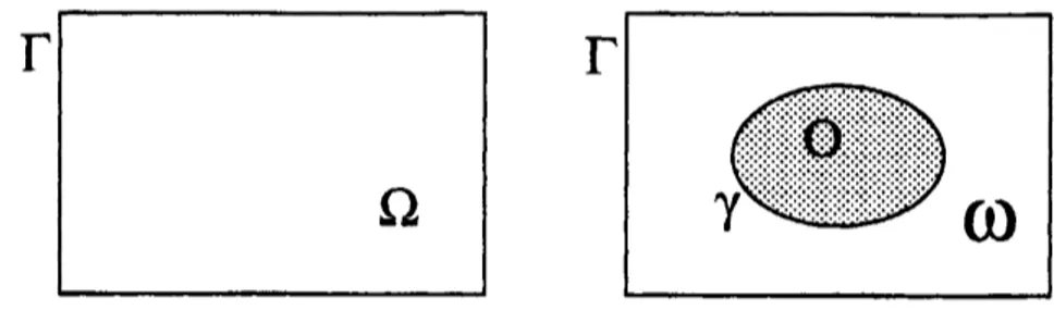
rectangular parallelepiped domain $\Omega$, the

fictitious

domain, such that

$\overline{O}\subset\Omega$, and then

we

set $\omega$ $=\Omega\backslash \overline{O}$ and $\Gamma$ $=\partial\Omega$ (see Figure 1). To approximate the

Sommerfeld

radiation

condition in (1),

we

impose the

Sommerfeld-like

boundary condition on $\Gamma$:

$\frac{\partial u}{\partial n}-iku=0$,

where $n$ is the outward unit normal vector to $\Gamma$. This boundary condition is not

so

accurate; however,

we

do not discuss

more

accurate

boundary

condition

here, for

which

we

refer the reader to [1], [10].

As

an

approximate problem to (1),

we

here

consider

the

following problem:

(2) $\{$

$-\Delta u-k^{2}u=0$ _in $\omega$,

$u=g$

on

$\gamma$,

$\frac{\partial u}{\partial n}-ik^{\wedge}u=$ $0$

on

$\Gamma$

.

数理解析研究所講究録 1320 巻 2003 年 37-46

We can equivalently rewrite (2) as asaddle point problem in $\Omega$ which is obtained by

extending the solution $u$ of (2) to $\Omega$

so

that the extended function also satisfies the

homogeneous Helmholtz equation in $O$, and by imposing weakly the non-homogeneous

Dirichlet boundary condition

on

$\gamma$ with aLagrange multiplier. When

we discretize

such

asaddle

point problem,

we

may

use

auniform

tetrahedral

mesh in $\Omega$;however,

we

need

to construct atriangular mesh

on

$\gamma$. These meshes

can

be constructed independently of

eachother, exceptthat the boundary meshsize is larger than the meshsize inthe domain.

Thus the mesh generation in the fictitious domain method is easier than that in the usual

finite element computations, especially when $\omega$ is acomplicated shape. When the $P_{1}$

conforming finite element

on

0and the $P_{0}$ finite element

on

$\gamma$

are

used, the constrain

matrixof the

discrete

saddle point problem, i.e., the matrix whose entries

are

integrals

of the product of basis functions ofthe $P_{1}$ and $P_{0}$ finite elements,

can

be automatically

computed with an algorithm introduced in Section 5. Furthermore, the use of uniform

meshes in $\Omega$ allows

us

to

use

fast Helmholtzsolvers

as

introduced in [3].

$\Gamma$

$\Gamma$

$\Omega$

co

Figure 1: Domains $\Omega$ and

$\omega$ etc.

We present

an

apriori

error

estimate for approximate solutions obtained by the

ficti-tious domain method. Such

an

apriori

error

estimate is derived by following

an

idea of

Girault and Glowinski [5]. Although they studied apositive definite Helmholtz problem,

we

here study

an

indefinite

one.

Thus

our

prooffor the

error

estimateis slightlydifferent

from theirs; however,

we

do not write it here, which will be

described

in aforthcoming

article. We further present results of numerical experiments concerning the rate of

con-vergence for approximate solutions of atest problem which confirm the obtained apriori

error

estimate.

Girault

et al. [6] analyze the

error

of the fictitious domain method applied to

anon-homogeneous steady incompressible

Navier-Stokes

problem. Bespalov [2],

Kuznetsov-Lipnikov [11], Heikkola et al. [9], [10] study another fictitious domain method, which

requires locally fitted meshes. Farhat et al. [4] propose afictitious domain decomposition

method aimed at solving efficientlypartially axisymmetric acoustic scattering problems. The remainder of this article is organized

as follows.

In

Section

2,

we

describe the fictitious domain

formulation

ofproblem (2) and present atheorem concerning the

well-posedness of the resulting saddle point problem. In

Section

3,

we

formulate adiscrete

problemofthe saddle point problem. In

Section

4,

we

present the apriori

error

estimate

mentioned above which

are

derived under

some

assumptions with respect to meshes in

$\Omega$ and

on

$\gamma$ and the regularity for the solution of the continuous saddle point problem.

In

Section

5,

we

describe how to compute the constrain matrix. In Section 6,

we

report

results of numerical experiments, which

are

consistent with the apriori

error

estimate.

2Fictitious domain

formulation

Aweak formulation of (2) is:

(3) $\{$

Find $u\in H^{1}(\omega)$ such that

$a(u, v)$ $=$ $0$ for all $v\in V$,

$u=g$

on

$\gamma$,

where $V=$

{

$v\in H^{1}(\omega)|v=0$ on

7}

and

$a(u, v)= \int_{\omega}(\nabla u\cdot\nabla\overline{v}-k^{2}u\overline{v})dx-ik\int_{\Gamma}u\overline{v}d\gamma$.

THEOREM 1for every $g\in H^{1/2}(\gamma)$, problem (3) has

a

unique solution.

We here introduce

some

notations. We denote the standard

Sobolev

space $H^{1}(\Omega)$ by

$X$. Let $H^{-1/2}(\gamma)$ be the set of all semi-lineax forms on $H^{1/2}(\gamma)$

.

We denote $H^{-1/2}(\gamma)$ by

$M$, and the duality pairing between $H^{-1/2}(\gamma)$ and $H^{1/2}(\gamma)$ by $\langle\cdot, \cdot\rangle_{\gamma}$

.

The solution of (3)

can

be obtained by solving the following saddle point problem:

(4) $\{$ $\mathrm{F}\lambda_{\frac{\}\in X}{b(v,\lambda)}}\cross\lambda f\mathrm{s}\mathrm{u}\mathrm{c}\mathrm{h}\frac{\frac{}{a}(u,v)\mathrm{i}\mathrm{n}\mathrm{d}\{u}{b(u,\mu)},+=0$

that

for all $v\in X$,

$=$ $\langle\mu, g\rangle_{\gamma}$ for all $\mu\in\Lambda f$,

where

$\tilde{a}(u, v)=\int_{\Omega}(\nabla u\cdot\nabla\overline{v}-k^{2}u\overline{v})dx-ik\int_{\Gamma}u\overline{v}d\gamma$ for $u$, $v\in X$,

$6(\mathrm{v}, \mu)=\overline{\langle\mu,v\rangle_{\gamma}}$ for $v\in X$ and for _{$\mu\in M$}

.

To describe the well-posedness ofproblem (4), we consider the following eigenvalue

prob-$\mathrm{l}\mathrm{e}\mathrm{m}$:

(5) $\{$

$-\Delta u$ $=$ $\alpha u$ in $O$, $u$ $=$ $0$

on

$\gamma$

.

We denote by athe set of all eigenvalues of (5).

THEOREM

2Assume

that $k^{2}\in(0, \infty)\backslash \sigma$

.

Then,

for

every $g\in H^{1/2}(\gamma)$, problem (4)

has

a

unique solution $\{u, \lambda\}\in H^{1}(\Omega)\cross H^{-1/2}(\gamma)$

.

Farther the restriction

of

$u$ to $\omega$ is the

solution

_of

problem (3).

3Discrete

problem

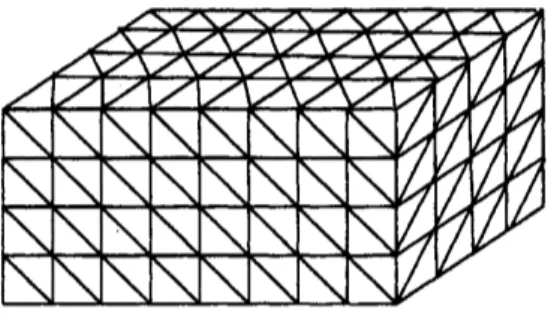
Wedivide $\Omega$ by auniform cube grid and

subdivide

each cubeinto sixtetrahedrons,

as

in

Figure

2.

Let $h$ denote the length of the longest edge of these tetrahedrons and let $\mathcal{T}_{h}$

denote the corresponding tetrahedrization of

0.

We

take

aCartesian

coordinate syste$\mathrm{m}$

in $R^{3}$

so

that $\Omega$

can

be represented

as

follows: $\Omega=(-l_{x}/2, l_{x}/2)\cross(-l_{y}/2, l_{y}/2)\cross$ $(-l_{z}/2, l_{z}/2)$. Let

$\mathcal{H}=\{h=\sqrt{3}h’|h’=\frac{l_{x}}{N_{x}}=\frac{l_{y}}{N_{y}}=\frac{l_{z}}{N_{z}}$, $(N_{x}, N_{y}, N_{\sim},)\in N^{3}\}$ .

We consider afamily $\{\mathcal{T}_{h}\}_{h\in \mathcal{H}}$ ofsuch tetrahedrizations of Q. For each $h\in \mathcal{H}$,

we

take

$X_{h}=$

{

$v_{h}\in C^{0}(\overline{\Omega})|v_{h}|_{T}\in P_{1}$ for every $T\in \mathcal{T}_{h}$

},

where $P_{1}$ denotes the space ofpolynomials, in three variables, of degree less than

or

equal

to

one.

Figure 2: Tetrahedrization of domain $\Omega$

.

We here

assume

(B) the boundary$\gamma$ is polyhedral, with restrictions

that

its angles at edges and vertices

are

not too small.

We divide each faceof$\gamma$ into triangular patches. Let $\eta$ be the maximumlength of the

sides ofthese triangular patches and denote by $P_{\eta}$ the corresponding triangulation of$\gamma$

.

We consider afamily $\{P_{\eta}\}_{0<\eta\leq\overline{\eta}}$of triangulations of $\gamma$. For each $\eta\in(0,\overline{\eta}]$,

we

take

$M_{\eta}=$

{

$\mu_{\eta}|\mu_{\eta}|p$ is aconstant for every $P\in P_{\eta}$

}.

Adiscrete problem of (4) is:

(6) $\{$ $\mathrm{F},\lambda_{\eta_{\frac{\}\in X_{h}\cross}{b(v_{h},\lambda_{\eta})}}}M_{\eta}\mathrm{s}\mathrm{u}\mathrm{c}\mathrm{h}\frac{\tilde{a}(u_{h},v_{h})\mathrm{i}\mathrm{n}\mathrm{d}\{u_{h}}{b(u_{h},\mu_{\eta})}+=0$

that

for all $v_{h}\in X_{h}$,

$=$ $\langle\mu_{\eta}, g\rangle_{\gamma}$ for all $\mu_{\eta}\in \mathrm{A}f_{\eta}$

.

4Error

estimate

We

assume

the following:

(HI) There exists apositive constant $\theta_{0}$ independent of $\eta\in(0,\overline{\eta}]$ such that $\theta_{P}\geq\theta_{0}$ for

all $P\in P_{\eta}$, where $0_{P}$ is the smallest angle of $P$

.

(HI) There exists apositive constant $L\cdot \mathrm{s}\mathrm{u}\mathrm{c}\mathrm{h}$ that _{$\eta\leq Lh$}

.

(H3) For every $P\in P_{\eta}$, the diameter ofthe inscribed circle of $P$ is grater than Ah.

For the solution $\{u, \lambda\}\in X\cross M$ of (4),

we

assume

(R1) There exists an $s\in(1/2,1]$ such that $u\in H^{1+s}(\Omega)$;

(R2) A $\in L^{\underline{9}}(\gamma)$.

We

now

consider the following auxiliary problem: for agiven $f\in L^{2}(\Omega)$, find $\{u, \lambda\}\in$ $H^{1}(\Omega)\mathrm{x}H^{-1/2}(\gamma)$ such that

(7) $\{$

$\tilde{a}^{*}(u, v)+\overline{b(v,\lambda)}=$ $(f, v)_{L^{2}(\Omega)}$ for all $v\in X$,

$6(\mathrm{v}, \mu)$ $=0$ for all $\mu\in M$,

where

$\tilde{a}^{*}(u, v)=\int_{\Omega}(\nabla u\cdot\nabla\overline{v}-k^{2}u\overline{v})dx+ik\int_{\Gamma}u\overline{v}d\gamma$

.

For every $f\in L^{2}(\Omega)$, problem (7) has aunique solution. We

assume

that for every

$f\in L^{2}(\Omega)$, the solution $\{u, \lambda\}\in X\cross M$ of (7) satisfies

(H3) $u\in H^{1+s}(\Omega)$, where $s$ is the constant presented in (R1);

(R4) $\lambda\in L^{2}(\gamma)$.

THEOREM 3Assume that hypotheses (B) and $(H1)-(H3)$ hold. Suppose that the

wave

number $k$

satisfies

$k^{B}\in(0, \infty)\backslash \sigma$ and that hypotheses $(R1)-(R4)$ hold. Then, there eist

positive constants $h-(k)$ and $\overline{\eta}(k)$ such that

for

all $\{h, \eta\}\in(0,\overline{h}(k))\cross(0,\overline{\eta}(k))$ , problem

(6) has a unique solution $\{u_{h}, \lambda_{\eta}\}\in X_{h}\mathrm{x}M_{\eta}$, and there exists

a

positive

constant

$C$ such

that

(8) $||u-u_{h}||_{H^{1}(\Omega)}+||\lambda-\lambda_{\eta}||_{H^{-1/2}}(\gamma)\leq C\{h^{\mathit{8}}||u||_{H^{1+s}(\Omega)}+\sqrt{\eta}||\lambda||_{L^{2}(\gamma)}\}$

.

5Numerical computation

Let $\varphi_{1}$, $\ldots$ , $\varphi N$ be the basis functions of $X_{h}$ such that $\varphi_{n}(Q_{l})=\delta_{nl}(1\leq n, l\leq N)$,

where$N$ $=\dim X_{h}$, $Q_{l}(1\leq l\leq N)$

are

the nodes of

tetrahedrization

$\mathcal{T}_{h}$, and $\delta_{nl}$ denotes

Kronecker’s delta. Also let$\psi_{1}$,

$\ldots$ ,$\psi_{M}$ be the basis functions of$M_{\eta}$ suchthat

$\psi_{m}|_{P_{\mathrm{t}}}\equiv\delta_{ml}$

$(1\leq m, l\leq \mathcal{M})$, where $\mathcal{M}=\dim M_{\eta}$ and $P_{l}(1\leq l\leq \mathcal{M})$

are

the triangular patches of

triangulation $P_{\eta}$

.

Then the solution {un, $\lambda_{\eta}$

}

of problem (6) is written

as

follows:

$u_{h}= \sum_{n=1}^{N}c_{n}\varphi_{n}$ and $\lambda_{\eta}=\sum_{m=1}^{\mathrm{A}1}d_{m}\psi_{m}$

with $(c_{n})_{1\leq n\leq N}\in C^{N}$ and $(d_{m})_{1\leq m\leq\lambda 4}\in C^{\mathcal{M}}$, and problem (6) is

reduced

to thefollowing

linearsystem:

$\{\begin{array}{ll}A B^{T}B O\end{array}\}\{\begin{array}{l}cd\end{array}\}=\{\begin{array}{l}og\end{array}\}$ ,

$A=(\tilde{a}(\varphi_{n}, \varphi_{l}))_{1\leq l,n\leq N}$, $B=(b(\varphi_{n}, \psi_{m}))1\leq m\leq\lambda 4,1\leq n\leq N$,

$c=(c_{n})_{1\leq n\leq N}$, $d=(d_{m})_{1\leq m\leq \mathcal{M}}$,

$g=(\overline{\langle\psi_{m},g\rangle_{\gamma}})_{1\leq m\leq \mathcal{M}}$

Computation of matrix $A$ is easy because uniform meshes

are

used in $\Omega$;however,

computation ofmatrix $B$ is not

so

easy at first glance, so

we

willexplain how to compute

matrix $B$ in the subsequent subsection.

5,1

_Computation

_of

_matrix

$B$

We first note that the $(n, m)$-entries of matrix $B$ are given by

$b( \varphi_{n}, \psi_{m})=\int_{P_{n\iota}}\varphi_{n}d\gamma$.

Tocomputethese valuesexactly,

we

needto construct atriangulationof theintersection of

triangular patch $P_{m}$ and eachoftetrahedral elements ofwhichthe support of$\varphi_{n}$ consists.

We give

an

algorithm for constructing such atriangulation. We fix atriangular patch $P$

and atetrahedral element $K$, which are considered to be closed sets.

Algorithm for constructing atriangulation of $P\cap K$:

1. Compute the plane $\Pi$ which includes the triangular patch $P$.

2. Seek $\Pi\cap K$ whose

measure

is positive.

2-1.

Count

the number $N_{0}$ of vertices of $K$ which

are on

$\Pi$ and the number $N_{+}$ of

vertices

of

$K$ which

are

above $\Pi$. The

cases

for $(\mathrm{i}\mathrm{V}\mathrm{o}, N_{+})$

are

listed in

Table 1.

2-2. Compute the intersection points of$\Pi$ and edges of_$K$ which

are

not vertices of

$K$. Their number $N_{i}$ is written in Table 1.

2-3. If$\Pi\cap K$ is atriangle, then proceed to the next procedure.

If $\Pi\cap K$ is aquadrangle, then divideit into two triangles and proceed to the

next procedure.

If the

measure

of $\Pi\cap K$ is zero, then the

measure

of $P\cap K$ is also zero, and hence need not construct atriangulation of$P\cap K$

.

Thus, if the

measure

of $\Pi\cap K$ is positive then

we

can

obtain

one or

two triangles,

which will be denoted by $T$ in the following, and

are

also

considered

to be closed

42

ble

1, not $K\mathrm{v}$

3.

Construct

atriangulation of$P\cap T$

.

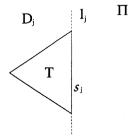
Let $s_{1}$, $s_{2}$, $s_{3}$ be the sides of the triangle $T$, and let $l_{j}(j=1,2,3)$ be the line including $s_{j}$. Let $D_{j}$ be the closed half-plane on $\Pi$ dividedby $l_{j}$ which includes the

vertex of$T$ not

on

$l_{j}$ (see Figure 3). We here note that we have

$T\cap P=(j=\cap^{3}D_{j})1\cap P=D_{3}\cap(D_{2}\cap(D_{1}\cap P))$.

Prom this relation, we get the following procedure for constructing atriangulation

of$T\cap P$.

3-1. Construct atriangulation of $D_{1}\cap P$

.

(a) Seek the line $l_{1}$.

(b) Count thenumber$n_{0}$ ofvertices of$P$whichare on

$l_{1}$ and the number_{$n_{+}$}of

vertices of$P$ which are interior points of $D_{1}$. There

are

cases

for $(n_{0}, n_{+})$

as

in Table 2.

(c) Compute the intersection points

of

$l_{1}$ and sides of$P$which

are

not vertices

of $P$

.

Their number $n_{i}$ is written in Table 2.

(d) If $D_{1}\cap P$ is atriangle, which will be

denoted

by $P_{1}$, then proceed to

procedure 3-2.

If $D_{1}\cap P$ is aquadrangle, then divide it into two triangles $P_{1}^{(1)}$ and $P_{1}^{(2)}$,

and proceed to procedure 3-2.

If the

measure

of $D_{1}\cap P$ is zero, then the

measure

of$T\cap P$ is also zero,

and hence need not construct atriangulation of$T\cap P$

.

$\Pi$

Figure3: Half-plane D$, triangle $T$, side $s_{j}$ and line $l_{j}$

.

Table 2: $D_{1}\cap P$ and the number $n_{i}$ of the intersection points of$l_{1}$ and sides of $P$ which

are

not vertices of $P$

are

listed for each $(n_{0}, n_{+})$, where no is the number of the vertices

of$P$ which are on $l_{1}$, and

$n_{+}$ is the number of the vertices of $P$ which

are

interior points

of $D_{1}$.

3-2. Construct atriangulation of $D_{2}\cap(D_{1}\cap P)$.

If$D_{1}\cap P$ is atriangle, then

we

have

$D_{2}\cap(D_{1}\cap P)=D_{2}\cap P_{1}$,

and hence apply procedure 3-1 to $D_{2}\cap P_{1}$.

If $D_{1}\cap P$ is aquadrangle, then we have

$D_{2}\cap(D_{1}\cap P)=(D_{2}\cap P_{1}^{(1)})\cup(D_{2}\cap P_{1}^{(2)})$,

and hence apply procedure 3-1 to $D_{2}\cap P_{1}^{(1)}$ and $D_{2}\cap P_{1}^{(2)}$

.

3-3.

Construct atriangulation of$D_{3}\cap(D_{2}\cap(D_{1}\cap P))=T\cap P$ in the

same

way

as

in procedure 3-2.

Implementing this algorithm in acomputer,

we can

automatically construct

atriangula-tion of$K\cap P$

.

6Numerical experiments

We

measure

convergence

rates of approximate solutions for atest problem whose exact

solution is known analytically. In the problem, the boundary $\gamma$ is aregular octahedron

with length of the edges equal to 1.5, $\Omega$ $=(-2,2)^{3}$, and the

wave

number $k=0.4$. The

test problem is:

$\{$ $\mathrm{F}\lambda\cross M\mathrm{s}\mathrm{u}\mathrm{c}\mathrm{h}\mathrm{t}\mathrm{h}\mathrm{a}\mathrm{t}\frac{\tilde{a}(u,v)\mathrm{i}\mathrm{n}\mathrm{d}\{u}{b(u,\mu)},+=\int_{\Omega}\frac{\}\in X}{b(v,\lambda)}F\overline{v}dx+\int_{\Gamma}f\overline{v}d\gamma$ for all $v\in X$,

$=$ $\langle\mu, g\rangle_{\gamma}$ for all $\mu\in M$,

where the data $F$, $f$ and $g$

are so

chosen that the exact solution becomes

$u(x, y, z)=x^{2}+y^{2}+z^{2}+i(x^{2}-y^{2}-z^{2})$ in $\Omega$,

which belongs to $C^{\infty}(\overline{\Omega})$, and thenthe Lagrange multiplier $\lambda=0$ since Ais given by

A $= \frac{\partial u|_{\omega}}{\partial\nu}-\frac{\partial u|_{\mathcal{O}}}{\partial\nu}$,

where $\nu$ is the unit normal vector to $\gamma$ outward from $O$. This problem is

associated

with

the following problem:

$\{$

$-\Delta u-k^{2}u$ $=$ $F$ in $\omega$,

$u$ $=$ $g$

on

$\gamma$,

$\frac{\partial u}{\partial n}-iku$ _{$=$ $f$}

on

$\Gamma$

.

Although

we

have considered the

case

where

$F=f=0$

in the above sections, all the

theorems stated above holdfor the

case

where$F$ and $f$

are

non-homogeneous, withproper

modifications.

In

our

numerical experiments, mesh sizes $h$ and $\eta$ satisfy

$h$, _{$\eta\leq(2\pi/k)/10$}, i.e., the

used meshes include at least ten grid points per the wavelength, which is acommonly

used criterion for computing appropriate numerical solutions of the Helmholtz problem.

In addition, the diameter of inscribed circle ofeach triangular patch is taken to be equal

to $4h$ in order that hypothesis $(\# 3)$ is satisfied. All computations

were

performed in

doubleprecision complexarithmetic

on

VT-Alpha6 $\mathrm{G}\mathrm{I}\mathrm{V}$personal computer $(\mathrm{A}\mathrm{l}\mathrm{p}\mathrm{h}\mathrm{a}21264$ $800\mathrm{M}\mathrm{H}\mathrm{z}$ CPU, $4\mathrm{G}\mathrm{B}$ Memory).

We report

errors

measured

with $H^{1}(\Omega)$-seminorm and $L^{2}(\Omega)$

-norm

in Table 3,

which

shows that the rates of convergence with respect to $H^{1}(\Omega)$-seminorm

and

$L^{2}(\Omega)$

-norm are

$O(h^{1})$ and $o(h^{2})$, respectively. This convergence rate with respect to $H^{1}(\Omega)$-seminorm is

consistent with

error

estimate (8) since $u\in H^{2}(\Omega)$ and $\lambda=0$ in this test problem.

References

[1] Bamberger, Alain; Joly, Patrick; Roberts, Jean E.:

Second-0rder

absorbing boundary

conditions for the

wave

equation: asolution for the

corner

problem.

SIAM J.

Numer. Anal.

27

(1990),

no.

2,

323-352

Table 3: Errors with respect to $H^{1}(\Omega)$-seminorm and $L^{2}(\Omega)$

-norm.

[2] Bespalov, A. N.: Application ofalgebraic fictitious domainmethod to the solution of

3D electromagnetic scattering problems. Russian J. Numer. Anal. Math. Modelling

12 (1997),

no.

3,

211-229.

[3] Elman, Howard C;O’Leary, Dianne P.: Efficient iterative solution of the

three-dimensional Helmholtz equation. J. Comput. Phys. 142 (1998), 163-181.

[4] Farhat, Charbel; Hetmaniuk, Ulrich: Afictitious domain decomposition method

for the solution of partially axisymmetric acoustic scattering problems. I. Dirichlet

boundary conditions. Internat. J. Numer. Methods Engrg. 54 (2002),

no.

9,

1309-1332.

[5] Girault, V.; Glowinski, R.: Error analysis of afictitious domain method applied to

a

Dirichlet problem. Japan J. Indust. Appl. Math. 12 (1995),

no.

3, 487-514.

[6] Girault, V.; Glowinski, R.; Lopez, H.; Vila,

J.-P.:

Aboundary $\mathrm{m}\mathrm{u}\mathrm{l}\mathrm{t}\mathrm{i}\mathrm{p}\mathrm{l}\mathrm{i}\mathrm{e}\mathrm{r}/\mathrm{f}\mathrm{i}\mathrm{c}\mathrm{t}\mathrm{i}\mathrm{t}\mathrm{i}\mathrm{o}\mathrm{u}\mathrm{s}$

domain methodfor thesteady incompressibleNavier-Stokesequations. Numer. Math.

88 (2001),

no.

1, 75-103.

[7] Glowinski, Roland; Pan, Tsorng-Whay; Periaux, Jacques: Afictitious domain

method for Dirichlet problem and applications. Comput. Methods Appl. Mech.

En-grg. I11 (1994), no. 3-4,

283-303.

[8] Glowinski, Roland; Pan, Tsorng-Whay; Periaux, Jacques: Afictitious domain

method for external incompressible viscousflow modeledby

Navier-Stokes

equations.

Finite

element methods in large-scale computational fluid dynamics (Minneapolis,

MN, 1992). Comput. Methods Appl. Mech. Engrg. 112 (1994), no. 1-4, 133-148.

[9] Heikkola, Erkki; Kuznetsov, YuriA.; Neittaanmaki, Pekka; Toivanen,

Jari:

Fictitious

domain methods for the numerical solution of tw0-dimensional scattering problems.

J. Comput. Phys.

145

(1998),

no.

1,

_89-109.

[10] Heikkola, Erkki; Kuznetsov, Yuri A.; Lipnikov, Konstantin N.: Fictitious domain

methods for thenumericalsolution of three-dimensionalacousticscattering problems.

J. Comput.

Acoust.

7(1999),

no.

3, 161-183.

[11] Kuznetsov,Yu. A.; Lipnikov, K. N.: 3D Helmholtz

wave

equationbyfictitious domain

method.

Russian

J.

Numer.

Anal. Math. Modelling

13

(1998),

no.

5,

371 -387