一般化された sine-Gordon 方程式の厳密解法 (非線形波動現象の多様性と普遍性)

一般化された

sine-Gordon

方程式の厳密解法

Exact method of solution for the generalized sine-Gordon equation

山口大学大学院理工学研究科 松野 好雅 (Yoshimasa Matsuno)

Division ofApplied Mathematical Science

Graduate School of

Science

and Engineering

Yamaguchi University

Abstract

We develop

a

direct method for solving the generalized sine-Gordon equation

$u_{tx}=(1+\partial_{x}^{2})\sin u$. Using the bilinear transformation method,

we

construct exact

multisoliton solutions and investigate their properties. In particular,

we

show that

the equationexhibits kinkand breathersolutions and does not admit multi-valued

solutions like loop solitons. We also demonstrate that the equation reduces to the

short pulse and sine-Gordon equations in appropriate scaling limits. The limiting

form of

the multisoliton solutions

are

also presented. Finally,

we

derive

an

infinite

number ofconservation laws by using

a

novel B\"acklund _{transformation connecting}

solutions of the sine-Gordon and generalized sine-Gordonequations.

1. Introduction

The generalized sine-Gordon $(sG)$ equation

$u_{tx}=(1+\nu\partial_{x}^{2})\sin u$, (1.1)

where $u=u(x, t)$ is

a

scalar-valued function, $\nu$ is

a

real parameter, $\partial_{x}^{2}=\partial^{2}/\partial x^{2}$

and the subscripts $t$

and

_$x$ appended to _$u$ denote partial differentiation, has been

derived by Fokas [1]. In the

case

of $\nu=-1$, its integrability

was

established

by constructing

a

Lax pair associated with it and the initial value problem

was

formulated for decaying initial data by

means

ofthe inverse scatteringmethod [2].

Quite recently,

we

developed asystematic method for solving equation (1.1) with

$\nu=-1$ _{and obtained soliton solutions in the form of parametric representation}

[3].

Here,

we

consider equation (1.1) with $\nu=1$

$u_{tx}=(1+\partial_{x}^{2})\sin u$. (1.2)

One

ofthe remarkable features ofequation (1.2) is that it does not admit

multi-valued solutions like loop solitons

as

obtained in the

case

of $\nu=-1$. The detail

2. Exact method of solution

2.1. Hodograph

_{transformation}

First,

we

introduce the

new

dependent variable $r$ in accordance with the relation

$r^{2}=1-u_{x}^{2}$, $(0<r<1)$, (2.1)

to transform equation (1.2) into the conservation law ofthe form

$r_{t}-(r\cos u)_{x}=0$

.

(2.2)

This expression makes it possible to define the hodograph transformation $(x, t)arrow$

$(y, \tau)$ by

$dy=rdx+r\cos udt$, $d\tau=dt$

.

(2.3)

The $x$ and $t$

derivatives

are

then rewritten in terms of the

$y$ and $\tau$ derivatives

as

$\frac{\partial}{\partial x}=r\frac{\partial}{\partial y}$, $\frac{\partial}{\partial t}=\frac{\partial}{\partial\tau}+r\cos u\frac{\partial}{\partial y}$

.

(2.4)

With the

new

variables $y$ and $\tau,$ $(2.1)$ and (2.2)

are

recast into the form

$r^{2}=1-r^{2}u_{y}^{2}$, (2.5)

$( \frac{1}{r})_{\tau}+(\cos u)_{y}=0$, (2.6)

respectively. FUrther reduction is possible if

one

defines the variable $\phi$ by

$u_{y}=\sinh\phi$, $\phi=\phi(y, \tau)$

.

(2.7)

It follows from (2.5) and (2.7) that

$\frac{1}{r}=\cosh\phi$. (2.8)

Substituting (2.7) and (2.8) into equation (2.6),

we

find

$\phi_{\tau}=\sin u$

.

(2.9)

If

we

eliminate the variable $\phi$ from (2.7) and (2.9),

we

obtain

a

single PDE for

$u$

$\frac{u_{\tau y}}{\sqrt{1+u_{y}^{2}}}=\sin u$

.

(210)

Similarly, elimination of the variable $u$ gives a single PDE for $\phi$

By inverting the hodograph transformation (2.3) and using (2.8), the equation

that determines the inverse mapping $(y, \tau)arrow(x, t)$ isfound to be governed by the

system of linear PDEs for $x=x(y, \tau)$

$x_{y}=\cosh\phi$, $(2.12a)$

$x_{\tau}=-\cos u$

.

$(2.12b)$

$2.2$. Bilinear

formalism

Let $\sigma$ and

$\sigma^{l}$ be solutions of the $sG$ equation

$\sigma_{\tau y}=\sin\sigma$, $\sigma=\sigma(y, \tau)$, $(2.13a)$

$\sigma_{\tau y}’=\sin\sigma’$, $\sigma’=\sigma’(y, \tau)$

.

$(2.13b)$

The solutions of the above equations

can

be put into the form

$\sigma=2i\ln\frac{f’}{f}$, $\sigma’=2i\ln\frac{g’}{g}$. $(2.14a, b)$

For soliton solutions, the tau functions $f,$$f’,$$g$ and $g’$ satisfy the following system

of bilinear equations:

$D_{\tau}D_{y}f \cdot f=\frac{1}{2}(f^{2}-f^{\prime 2})$, $D_{\tau}D_{y}f’ \cdot f’=\frac{1}{2}(f^{;2}-f^{2})$, $(2.15a, b)$

$D_{\tau}D_{y}g \cdot g=\frac{1}{2}(g^{2}-g^{\prime 2})$, $D_{\tau}D_{y}g’ \cdot g’=\frac{1}{2}(g^{\prime 2}-g^{2})$, $(2.16a, b)$

where the bilinear operators $D_{\tau}$ and $D_{y}$

are

defined by

$D_{\tau}^{m}D_{y}^{n}f\cdot g=(\partial_{\tau}-\partial_{\tau’})^{m}(\partial_{y}-\partial_{y’})^{n}f(\tau, y)g(\tau’, y’)|_{\tau’=\tau,y’=y}$, $(m, n=0,1,2, \ldots)$

.

(2.17)

Now,

we

seek solutions of equations (2.7) and (2.9) of the form

$u= i\ln\frac{F’}{F}$, $\phi=\ln\frac{G’}{G}$, $(2.18a, b)$

where $F,$$F’,$$G$ and $G’$

are new

tau functions. If

we

impose the condition

$F’F=G’G$, (219)

among these tau functions, then equations (2.7) and (2.9)

can

be transformed to

the following bilinear equations

$iD_{\tau}G’\cdot G=\frac{1}{2}(F^{2}-F^{\prime 2})$, (2.21)

respectively. The proposition below provides the tau functions $F,$$F’,$ $G$ and $G’$ in

terms of $f,$$f’,$$g$ and $g^{l}$

.

Proposition 2.1.

_If

we

impose the conditions

_for

the $tau$

functions

$f,$$f’,$$g$ and$g’$

$iD_{y}f\cdot g’=\frac{1}{2}(fg’-f’g)$, $iD_{y}f’\cdot g=\frac{1}{2}(f’g-fg’)$, _{$(2.22a, b)$} $iD_{\tau}f\cdot g=-\frac{1}{2}(fg-f’g’)$, $i$D..$f’ \cdot g’=-\frac{1}{2}(f’g’-fg)$,

$(2.23a, b)$

then the solutions

_of

bilinear equations (2.20) and (2.21) subjected to the condition

(2. 19) are given by

$F=fg$, $F’=f’g’$, $(2.24a)$

$G=fg’$, $G’=f’g$

.

$(2.24b)$

2.3. Pammetric representation

Proposition 2.2. $\cosh\phi$ is given in terms

of

the $tau$

functions

$f,$$f’,$$g$ and$g’$

as

$\cosh\phi=1+i(\ln\frac{g’g}{f’ f})_{y}$

.

(2.25)

Integrating (2.12a) with (2.25) by $y$ yields the expression of $x$

$x=y+ i\ln\frac{g’g}{f’ f}+d(\tau)$, (2.26)

where $d$ is

an

integration constant which depends generally

on

$\tau$

.

The expression

(2.26) now leads to

our

main result:

Theorem 2.1. The solution

_of

equation (1.2) can be expressed by the parametric

representation

$u(y, \tau)=i\ln\frac{f’g’}{fg}$, _$(2.27a)$

$x(y, \tau)=y-\tau+i\ln\frac{g’g}{ff}+y_{0}$, $(2.27b)$

where the $tau$

functions

$f,$$f’,$$g$ and $g’$ satisfy equations (2.15), (2.16), (2.22) and

(2.23) and $y_{0}$ is

an

arbitrary constant independent

of

$y$ and $\tau$.

An interesting feature of the parametric solution (2.27) is that it never exhibits

singularities

as

encountered in the

case

of equation (1.1) with $\nu=-1$

.

Indeed

showing that $u_{x}$ always takes

a

finite value.

2.4.

Multisoliton solutions

Theorem 2.2. The

_{tau-functions}

$f,$$f’,$$g$ and$g’$ givcn bclow satisfy both the

bilin-ear

_forms

(2.15) and (2.16)

_of

the $gG$ equation and the bilinear equations (2.22)

and (2.23),

$f= \sum_{\mu=0,1}\exp[\sum_{j=1}^{N}\mu_{j}(\xi_{j}+d_{j}+\frac{\pi}{2}i)+\sum_{1\leq j<k\leq N}\mu_{j}\mu_{k}\gamma_{jk}]$ , $(2.29a)$

$f’= \sum_{\mu=0,1}\exp[\sum_{j=1}^{N}\mu_{j}(\xi_{j}+d_{j}-\frac{\pi}{2}i)+\sum_{1\leq j<k\leq N}\mu_{j}\mu_{k}\gamma_{jk}]$ , $(2.29b)$

$g= \sum_{\mu=0,1}\exp[\sum_{j=1}^{N}\mu_{j}(\xi_{j}-d_{j}+\frac{\pi}{2}i)+\sum_{1\leq j<k\leq N}\mu_{j}\mu_{k}\gamma_{jk}]$ , $(2.30a)$

$g’= \sum_{\mu=0,1}\exp[\sum_{j=1}^{N}\mu_{j}(\xi_{j}-d_{j}-\frac{\pi}{2}i)+\sum_{1\leq j<k\leq N}\mu_{j}\mu_{k}\gamma_{jk}]$ , $(2.30b)$

where

$\xi_{j}=p_{j}y+\frac{1}{p_{j}}\tau+\mathscr{F}0$, $(j=1,2, \ldots, N)$, $(2.31a)$

$e^{\gamma_{jk}}=(\frac{p_{j}-p_{k}}{p_{j}+p_{k}})^{2}$, $(j, k=1,2, \ldots, N;j\neq k)$, $(2.31b)$

$e^{d_{j}}=\sqrt{\frac{1+\mathscr{A}_{j}}{1-ip_{j}}}$, $(j=1,2, \ldots, N)$

.

$($

2.31

$c)$

Here, $p_{j}$ and $\xi_{j0}$

are

arbitmry complex pammeters satisfying the conditions $p_{j}\neq$

$\pm p_{k}$

for

$j\neq k,$ $i=\sqrt{-1}$ and $N$ is

an

arbitmry positive integer. The notation

$\sum_{\mu=0,1}$ implies the summation

over

all possible combination

of

$\mu_{1}=0,1,$$\mu_{2}=$

$0,1,$ $\ldots,$$\mu_{N}=0,1$.

The parametric solution (2.27) with (2.29) and (2.30) is characterized by the $2N$

complexparameters$p_{j}$ and$\xi_{j0}(j=1,2, \ldots, N)$

.

It producesin general the

complex-valued solutions. The real-valued solutions

are

obtainable if

one

imposes certain

conditions

on

these parameters. Actually, there arise various type of solutions

depending

on

values of the parameters. These solutions include kinks, antikinks

and breathers. Among them,

we

consider following three types:

First, let $p_{j}$ and $\mathscr{F}o(j=1,2, \ldots, N)$ be real quantities. Then $f’=g^{*}$ and $g’=f^{*}$

and (2.27) _becomes

$u(y, \tau)=i\ln\frac{f^{*}g^{*}}{fg}$, $x(y, \tau)=y-\tau+i\ln\frac{f^{*}g}{fg^{*}}+y_{0}$

.

$(2.32a, b)$

Type 2; _{Breather solution}

We put $N=2M$ _where $M$ is

a

positive integer, and specify the parameters$p_{j}$ and

$\xi_{j,0}(j=1,2, \ldots, 2M)$

as

$p_{2j-1}=p_{2j}^{*}$, $\xi_{2j-1,0}=\xi_{2j,0}^{*}$, $(j=1,2, \ldots, M)$. (2.33)

It turns out that $f’=g^{*}$ and $g’=f^{*}$. Then, the solution

can

be written in the

same form as (2.32).

Type 3: Kink-breather solution

Let $N=2M+M’$ where $M$ and $M’$

are

positive integers. In addition to the

parameterization given by (2.33), the 2$M’$ parameters$p_{j}(>0)$ and $\xi_{j0}(j=2M+$

$1,2M+2,$ $\ldots,$$2M+M^{l})$

are

chosen to be real. Then, the parameteric solution

(2.32) represents the solution describing the interaction among $M$ breathers and

$M^{l}$ kinks. The antikink-breather solution

can

be constructed similarly.

For the above three types of solutions, $\phi$ from (2.18b) and

$u_{x}$ from (2.28) can

be given explicitly in terms of the tau functions $f,$$g$ and their complex conjugate

as

$\phi=\ln\frac{g^{*}g}{f^{*}f}$, (2.34)

$u_{x}= \frac{(g^{*}g)^{2}-(f^{*}f)^{2}}{(g^{*}g)^{2}+(f^{*}f)^{2}}$

.

(2.35)

Note that (2.34) provides real solutions of equation (2.11).

3. Properties ofsolutions

3.1. l-soliton solutions

The tau-functions for the l-soliton solutions

are

given by (2.29) and (2.30) with

$N=1$:

$f=1+ie^{\xi_{1}+d_{1}}$, $g=1+ie^{\xi_{1}-d_{1}}$, _{$(3.1a, b)$}

$\xi_{1}=p_{1}y+\frac{\tau}{p_{1}}+\xi_{10}$, $e^{d_{1}}=\sqrt{\frac{1+ip_{1}}{1-ip_{1}}}$

.

$(3.1c)$

The real parameters $p_{1}$ and $\xi_{10}$

are

related to the amplitude and phase of the

soliton, respectively and $\xi_{1}$ is the phase variable characterizing the solution. The

parametric representation of the solution (2.32)

can

be written in the form

$x=y-\tau+2\tan^{-1}(p_{1}\tanh\xi_{1})+2\tan^{-1}p_{1}+y_{0}$. $(3.2b)$

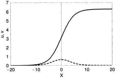
Figure 1 shows

a

typical profile of the kink solution

as a

function of $X$ together

with the corresponding profile of$v\equiv u_{x}$

.

$-20$ $-10$ $0$ 10 20

X

Figure 1 The profile of a kink $u$ (solid line) and corresponding profile of $v\equiv u_{X}$

(broken line). The parameter $p_{1}$ is set to

0.4

and the parameter $y_{0}$ is chosen such

that the center position of $u_{X}$ is at $X=0$

.

Here, $X=x+c_{1}t+x_{0},$ $c_{1}=1/p_{1}^{2}+1$

.

3.2. 2-soliton solutions

The tau-functions for the 2-soliton solutions read from (2.29) and (2.30) with

$N=2$ in the form

$f=1+i(e^{\xi_{1}+d_{1}}+e^{\xi_{2}+d_{2}})-\delta e^{\xi_{1}+\xi_{2}+d_{1}+d_{2}}$, $g=1+i(e^{\xi_{1}-d_{1}}+e^{\xi_{2}-d_{2}})-\delta e^{\xi_{1}+\xi_{2}-d_{1}-d_{2}}$,

$(3.3a, b)$

$\xi_{j}=p_{j}y+\frac{\tau}{p_{j}}+\xi_{j0}$, $e^{d_{j}}=\sqrt{\frac{1+ip_{j}}{1-ip_{j}}}$ $(j=1,2)$, $\delta=\frac{(p_{1}-p_{2})^{2}}{(p_{1}+p_{2})^{2}}$. $(3.3c)$

The parametric solution (2.32) with (3.3) represents three types of solutions,

de-pending on values of the parameters $p_{j}$ and $\xi_{0j}(j=1,2)$, i.e., kink-kink,

kink-antikink and breather solutions.

3.2.1. Kink-kink solution

If we specify $p_{1}$ and $p_{2}$ be positive and $\xi_{01}$ and $\xi_{02}$ be real, then the kink-kink

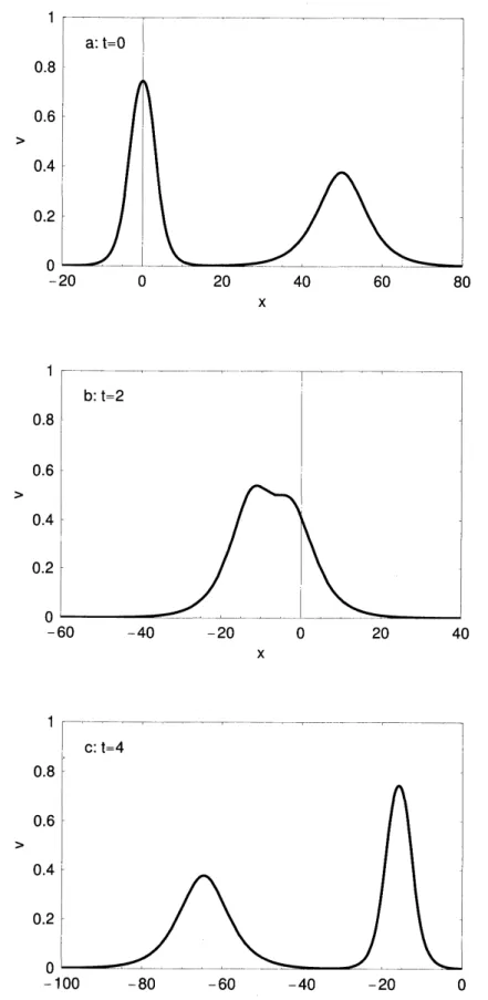
solution is obtained. The solution represents the so-called $4\pi$ kink. In figure

2a-$c$, we depict

a

typical profile of $v(\equiv u_{x})$ instead of $u$ for three different times.

It represents the interaction of two solitons with the amplitudes $A_{1}=0.38$ and

$-20$ $0$ 20 40 $x$ 60 $-60$ $-40$ $-20$ $0$ 20 40 $x$ $-100$ -SO $-60$ $-40$ $-20$ $0$ $x$

Figure 2

a-c

Theprofile of

a

two-soliton solution$v\equiv u_{x}$ for three different times,

a:

$t=0,$ $b:t=2,$

$c:t=4$

. The parameters

are

chosen

as

$p_{1}=0.2,$ $p_{2}=$

The formula for the phase shift arzsing from the interaction of two solitons is

given

as

follows:

$\Delta_{1}=-\frac{1}{p_{1}}\ln(\frac{p_{1}-p_{2}}{p_{1}+p_{2}})^{2}+4\tan^{-1}p_{2}$, $\triangle_{2}=\frac{1}{p_{2}}\ln(\frac{p_{1}-p_{2}}{p_{1}+p_{2}})^{2}-4\tan^{-1}p_{1}$

.

$(3.4a, b)$

It

can

be verified from (3.4) that $\Delta_{1}>0$ and $\Delta_{2}<0$ for _{$0<p_{1}<p_{2}$}

.

In the

present example,

formula

(3.4) yields $\Delta_{1}=10.3$ and $\Delta_{2}=-4.2$

.

3.2.2. Bruather solution

The breather solution

can

be constructed following the parameterization given by

(2.33). For $M=1$, _let

$p_{1}=a+ib$, $p_{2}=a-ib=p_{1}^{*}$, $(a>0, b>0)$, $(3.5a)$

$\xi_{10}=\lambda+i\mu$, $\xi_{20}=\lambda-i\mu=\xi_{10}^{*}$. $(3.5b)$

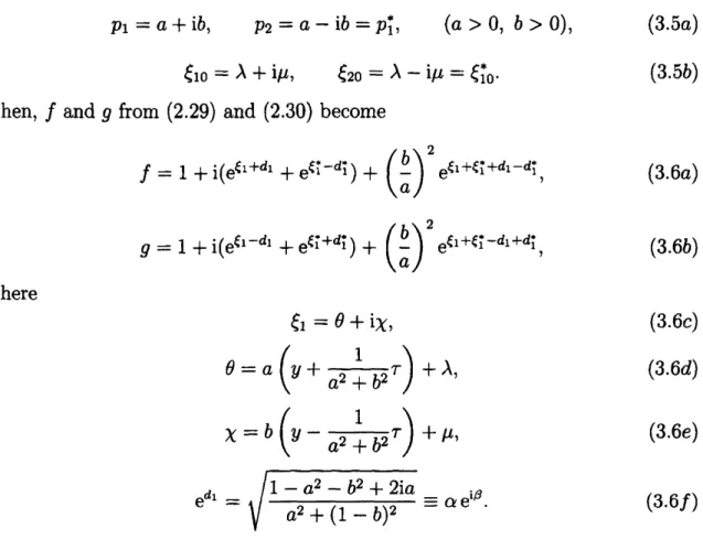
Then, $f$ and $g$ from (2.29) and (2.30) become

$f=1+ i(e^{\xi_{1}+d_{1}}+e^{\xi i-d}i)+(\frac{b}{a})^{2}e^{\xi_{1}+\epsilon i+d_{1}-d};$, _$(3.6a)$

$g=1+ i(e^{\xi_{1}-d_{1}}+e^{\xi i+d};)+(\frac{b}{a})^{2}e^{\xi_{1}+\xi_{1}^{*}-d_{1}+d;}$, _$(3.6b)$ where $\xi_{1}=\theta+i\chi$, $(3.6c)$ $\theta=a(y+\frac{1}{a^{2}+b^{2}}\tau)+\lambda$, $(3.6d)$ $\chi=b(y-\frac{1}{a^{2}+b^{2}}\tau)+\mu$, $(3.6e)$ $e^{d_{1}}=\sqrt{\frac{1-a^{2}-b^{2}+2ia}{a^{2}+(1-b)^{2}}}\equiv\alpha e^{i\beta}$. $(3.6f)$

$-40$ $-20$ $0$ $x$ 20 40 $-60$ $-40$ $-20x$ $0$ 20 $-80$ $-60$ $-40x$ $-20$ $0$

Figure 3

a-c

The profile of

a

breather solution for three different times, a:

$t=$ O, b: _{$t=5,$ $c:t=10$}. The _parameters

are

_chosen

as

_{$p_{1}=0.3+0.5i,$ $p_{2}=$}

3.3.

N-soliton solutions

3.3.1. N-kink solution

Let the velocity ofthe jth kink be$c_{j}=(1/p_{j}^{2})+1(p_{j}>0)$and order the magnitude

of the velocity of each kink

as

$c_{1}>c_{2}>\ldots>c_{N}$

.

We observe the interaction of $N$

kinks in

a

moving frame with

a

constant velocity $c_{\eta}$. We take the limit $tarrow-$

oo

with the phase variable $\xi_{n}$ being fixed. Then

$u\sim 2\tan^{-1}[\sqrt{1+p_{n}^{2}}\sinh(\xi_{n}+\delta_{n}^{(-)})]+\pi$, $(3.7a)$

$x \sim y-\tau+2\tan^{-1}[p_{n}\tanh(\xi_{n}+\delta_{n}^{(-)})]+4\sum_{j=n+1}^{N}\tan^{-1}p_{j}+2\tan^{-1}p_{n}+y_{0}$

.

$(3.7b)$

As $tarrow+\infty$, the expressions corresponding to (3.7)

are

given by

$u\sim 2\tan^{-1}[\sqrt{1+p_{n}^{2}}\sinh(\xi_{n}+\delta_{n}^{(+)})]+\pi$, $(3.8a)$

$x \sim y-\tau+2\tan^{-1}[p_{n}\tanh(\xi_{n}+\delta_{n}^{(+)})]+4\sum_{j=1}^{n-1}\tan^{-1}p_{j}+2\tan^{-1}p_{n}+y_{0}$ . $(3.8b)$

where

$\delta_{n}^{(+)}=\sum_{j=1}^{n-1}\ln(\frac{p_{n}-p_{j}}{p_{n}+p_{j}})^{2}$ , $($

3.8

_$c)$

$\delta_{n}^{(-)}=\sum_{j=n+1}^{N}\ln(\frac{p_{n}-p_{j}}{p_{n}+p_{j}})^{2}$, $(3.8d)$

$\delta_{n}=n+\cdot\prod_{\leq j<k\leq N}(\frac{p_{j}-p_{k}}{p_{j}+p_{k}})^{2}$

.

$(3.8e)$

Let $x_{c}$ be the center position of the nth kink in the $(x, t)$ coordinate system. As

$tarrow-\infty$

$x_{c}+ c_{n}t+x_{n0}\sim-\frac{1}{p_{n}}\delta_{n}^{(-)}+4\sum_{j=n+1}^{N}\tan^{-1}p_{j}+y_{0}$ , (3.9)

where $x_{n0}=\xi_{n0}/p_{n}-2\tan^{-1}p_{n}$

.

As $tarrow+\infty$,

on

the other hand, the

correspond-ing expression turns out to be

$x_{c}+c_{n}t+x_{n0} \sim-\frac{1}{p_{n}}\delta_{n}^{(+)}+4\sum_{j=1}^{n-1}\tan^{-1}p_{j}+y_{0}$. (3.10)

If

we

take into account the fact that all kinks propagate to the left,

we

can

define

the phase shift of the nth kink

as

Using (3.8c), (3.8d), (3.9) and (3.10),

we

find that

$\Delta_{n}=\frac{1}{p_{n}}\{\sum_{j=1}^{n-1}\ln(\frac{p_{n}-p_{j}}{p_{n}+p_{j}})^{2}-\sum_{j=n+1}^{N}\ln(\frac{p_{n}-p_{j}}{p_{n}+p_{j}})^{2}\}$

$+4 \sum_{j=n+1}^{N}\tan^{-1}p_{j}-4\sum_{j=1}^{n-1}\tan^{-1}p_{j}$, $(n=1,2, \ldots, N)$. (3.12)

3.3.2. M-breather

solution

We specify the parameters in (2.29) and (2.30) for the tau-functions $f$ and $g$

as

$p_{2j-1}=p_{2j}^{*}\equiv a_{j}+ib_{j}$, $a_{j}>0$, $b_{j}>0$, $(j=1,2, \ldots, M)$, $(3.13a)$

$\xi_{2j-1,0}=\xi_{2j,0}^{*}\equiv\lambda_{j}+i\mu_{j}$, $(j=1,2, \ldots, M)$. $(3.13b)$

Then, the phase variables $\xi_{2j-1}$ and $\xi_{2j}$

are

written

as

$\xi_{2j-1}=\theta_{j}+i\chi_{j}$, $(j=1,2, \ldots, M)$, $(3.14a)$

$\xi_{2j}=\theta_{j}-i\chi_{j}$, $(j=1,2, \ldots, M)$, $(3.14b)$

with the real phase variables

$\theta_{j}=a_{j}(y+c_{j}\tau)+\lambda_{j}$, $(j=1,2, \ldots, M)$, _$(3.14c)$

$\chi_{j}=b_{j}(y-c_{j}\tau)+\mu_{j}$, $(j=1,2, \ldots, M)$, $(3.14d)$

$c_{j}= \frac{1}{a_{j}^{2}+b_{j}^{2}}$, $(j=1,2, \ldots\dot{\prime}M)$

.

$(3.14e)$

The parametric solution (2.32) with (3.13) and (3.14) describes multiple

colli-sions of $M$ breathers.

3.3.3 Kink-breather solution

We take

a

3-soliton solution with parameters $p_{j}$ and $\xi_{0j}(j=1,2,3)$. If

one

impose the conditions that $p_{2}=p_{1}^{*},$$\xi_{02}=\xi_{01}^{*}$

as

already specified for the breather

solution and$p_{3}(>0),$ $\xi_{03}$ real for the kink solution, then the expression of_$u$ would

represent

a

solution describing the interaction between a kinkand

a

breather. The

tau functions $f$ and $g$

now

become

$f=1+ i(s_{1}e^{\xi_{1}}+\frac{1}{s_{1}}*e^{\xi i}+s_{3}e^{\xi_{3}})+(\frac{b}{a})^{2}\frac{s_{1}}{s_{1}}*e^{\xi_{1}+\xi_{1}^{*}}$

$g=1+ i(\frac{1}{s_{1}}e^{\xi_{1}}+s_{1}^{*}e^{\xi i}+\frac{1}{s_{3}}e^{\xi_{3}})+(\frac{b}{a})^{2}\frac{s_{1}^{*}}{s_{1}}e^{\xi_{1}+\xi_{1}^{*}}$

$- \frac{\delta_{13}}{s_{1}s_{3}}e^{\xi_{1}+\xi_{3}}-\delta_{13}^{*}\frac{s_{1}^{*}}{s_{3}}e^{\xi i+\xi_{3}}+i(\frac{b}{a})^{2}\frac{s_{1}^{*}}{s_{1}s_{3}}\delta_{13}\delta_{13}^{*}e^{\xi_{1}+\xi i+\xi_{3}}$ .

where

$(3.15b)$

$s_{1}= e^{d_{1}}=\sqrt{\frac{1-b+ia}{1-b-ia}}=\frac{1}{s_{2}}*$, $s_{3}=\sqrt{\frac{1+ip_{3}}{1-ip_{3}}}$, $\delta_{13}=(\frac{a-p_{3}+ib}{a+p_{3}+ib})^{2}=\delta_{23}^{*}$

.

$(3.15c)$

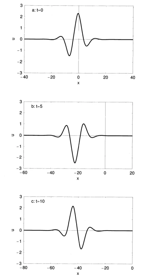
Figure 4a-c shows

a

typical profile of $v\equiv u_{x}$ for three different times. We

see

that the soliton overtakes the breather whereby it suffers

a

phase shift. Actually,

one has for $p_{3}^{2}<a^{2}+b^{2}$

$\Delta=\frac{2}{p_{3}}\ln\frac{(p_{3}+a)^{2}+b^{2}}{(p_{3}-a)^{2}+b^{2}}+4\tan^{-1}\frac{2a}{1-a^{2}-b^{2}}$, $(3.16a)$

and for $a^{2}+b^{2}<p_{3}^{2}$

$\triangle=-\frac{2}{p_{3}}\ln\frac{(p_{3}+a)^{2}+b^{2}}{(p_{3}-a)^{2}+b^{2}}-4\tan^{-1}\frac{2a}{1-a^{2}-b^{2}}$

.

$(3.16b)$

In the present example, formula (3.16a) gives $\triangle=7.7$

.

$-50$ $0$ 50 100 150

$-200$ $-150$ $-100$ $-50$ $0$

$x$

$-300$ $-250$

$-200x$ $-150$ $-100$

Figure 4

a-c

Theprofile of$v\equiv u_{x}$ forthree differenttimes which representsthe

interaction between

a

soliton and

a

breather,

a:

$t=$ O, b: $t=15,$ $c:t=30$

.

The

parameters are chosen

as

$p_{1}=0.2+0.4i,$ $p_{2}=p_{1}^{*}=0.2-0.4i,$ $p_{3}=0.3,$ $\xi_{10}=$

$\xi_{20}=0,$ $\xi_{30}=-30$

.

3.3.4

Breather-breather solution

The breather-breather (or 2-breather) solution isreduced from

a

4-soliton solution.

Figure 5a-c shows

a

typical profile of $u$ for three different times. It represents

a

typical feature

common

to the interaction of solitons, i.e., each breather

recovers

2 1 コ $0$ $-1$ $-2-100$ $0$ 100 $–$ $—200^{---}300$ $x$ 2 $—————————$ 1 コ $0$ $-1$ $-2-400$ $-300$ -200 $x$ $–100$ $—0$ $-600$ $-500$ -400 $x$ $-300$ $-200$

Figure $5a-c$The profile of

a

breather-breather solution $u$for threedifferent times,

a:

$t=$ O, b: $t=15,$ $c:t=30$

.

The parameters

are

chosen

as

$p_{1}=0.1+0.2i,p_{2}=$

$p_{1}^{*}=0.1-0.2i,p_{3}=0.15+0.3i,$ $p_{4}=p_{3}^{*}=0.15-0.3i,$ $\xi_{10}=\xi_{20}^{*}=-15,$ $\xi_{30}=$

4. Reduction to the short pulse and $sG$ equations

We write the short pulse equation in the form

$u_{tx}=u- \frac{\nu}{6}(u^{3})_{xx}$, (4.1)

where $u=u(x, t)$ represents the magnitude of the electric field and $\nu$ is a real

constant. The short pulse equation (4.1) with $\nu=-1$ was _proposed

as

a _model

nonlinear equationdescribing the propagation of ultra-short optical pulses in

non-linear media [5]. Quite recently, equation (4.1) with $\nu=1$

$u_{tx}=u- \frac{1}{6}(u^{3})_{xx}$, (4.2)

was

shown to modeltheevolution of ultra-short pulses inthe band gap of nonlinear

metamaterials [6]. See [7] for

a

review

on

exactsolutions oftheshortpulseequation

and related topics.

4.1.

Reduction to the short pulse equation

4.1.1.

Scaling limit

_of

the genemlized $sG$ equation

Let

us

first introduce

new

variables with bar according to the relations

$\overline{u}=\frac{u}{\epsilon}$, $\overline{x}=\frac{1}{\epsilon}(x+t)$, $\overline{y}=\frac{y}{\epsilon}$ $\overline{y}_{0}=\frac{y_{0}}{\epsilon}$, $\overline{t}=\epsilon t$, $\overline{\tau}=\epsilon\tau$,

$\overline{p}_{j}=\epsilon p_{j}$, $\overline{\xi}_{j0}=\mathscr{F}0$, $(j=1,2, \ldots, N)$, (4.3)

where $\epsilon$ is

a

small parameter and the quantities with bar are assumed to be order

1. Rewriting equation (1.2) in terms of the

new

variables and expanding$\sin\epsilon\overline{u}$ in

an infinite series with respect to $\epsilon$ and comparing terms oforder $\epsilon$ on both sides,

we

obtain equation (4.2) written by the

new

variables.

Under the scaling (4.3), expression (2.7) is invariant and hence

we

put $\overline{\phi}=\phi$ to

give

$\overline{u}_{\overline{y}}=\sinh\overline{\phi}$. (4.4)

Equation (2.9) then reduces to

$\overline{\phi}_{\overline{\tau}}=\overline{u}$

.

(4.5)

Equations (2.10) and (2.11) now become

$\frac{\overline{u}_{\overline{\tau y}}}{\sqrt{1+\overline{u}_{y}^{2}}}=\overline{u}$ (4.6)

$\overline{\phi}_{\overline{\tau y}}=\sinh\overline{\phi}$, (4.7)

4.1.2.

Scaling limit

_of

the N-soliton solution

The expansion ofthe tau function $f$ is given by

$f= \sum_{\mu=0,1}(1-i\epsilon\sum_{j=1}^{N}\frac{\mu_{j}}{\overline{p}_{j}})\exp[\sum_{j=1}^{N}\mu_{j}(\overline{\mathscr{F}}+\pi i)+\sum_{1\leq j<k\leq N}\mu_{j}\mu_{k}\overline{\gamma}_{jk}]+O(\epsilon^{2})$

$=\overline{f}-i\epsilon\overline{f}_{\overline{\tau}}+O(\epsilon^{2})$, (4.8a)

where

$\overline{f}=\sum_{\mu=0,1}\exp[\sum_{j=1}^{N}\mu_{j}(\overline{\mathscr{F}}+\pi i)+\sum_{1\leq j<k\leq N}\mu_{j}\mu_{k}\overline{\gamma}_{jk}]$ , $(4.8b)$

$\overline{\mathscr{F}}=\overline{p}_{j}\overline{y}+\frac{\overline{\tau}}{\overline{p}_{j}}+\overline{\xi}_{j0}$, $(j=1,2, \ldots, N)$, $(4.8c)$

$e^{\overline{\gamma}_{jk}}=(\frac{\overline{p}_{j}-\overline{p}_{k}}{\overline{p}_{j}+\overline{p}_{k}})$ , $(j, k=1,2, \ldots, N;j\neq k)$

.

$(4.8d)$

Similarly

$f’=\overline{g}-i\epsilon\overline{g}_{\overline{\tau}}+O(\epsilon^{2})$, $g=\overline{g}+i\epsilon\overline{g}_{\overline{\tau}}+O(\epsilon^{2})$, $g’=\overline{f}+i\epsilon\overline{f}_{\overline{\tau}}+O(\epsilon^{2}),$ $(4.9a, b, c)$

with

$\overline{g}=\sum_{\mu=0,1}\exp[\sum_{j=1}^{N}\mu_{j}\overline{\xi}_{j}+\sum_{1\leq j<k\leq N}\mu_{j}\mu_{k}\overline{\gamma}_{jk}]$. $(4.9d)$

The parametric solution of the short pulse equation (4.2) in terms of the tau

functions $\overline{f}$ and

$\overline{g}$ is given

as

follows:

$\overline{u}=2(\ln\frac{\overline{g}}{\frac{}{f}})_{\overline{\tau}}$ , $\overline{x}=\overline{y}-2(\ln\overline{f}\overline{g})_{\overline{\tau}}+\overline{y}_{0}$

.

$(4.10a, b)$

4.2.

Reduction

to

the $sG$ equation

If

we

introduce the following

new

scaled variables

$\overline{u}=u$, $\overline{x}=\epsilon x$, $\overline{y}=\epsilon y$, $\overline{t}=\frac{t}{\epsilon}$, $\overline{\tau}=\frac{\tau}{\epsilon}$,

$\overline{p}_{j}=\frac{p_{j}}{\epsilon}$, $\overline{\xi}_{j0}=\xi_{j0},$ $(j=1,2, \ldots, N)$, (4.11)

then in the limit of $\epsilonarrow 0$,

we can

deduce the generalized _$sG$ equation (1.2) to the

$sG$ equation

The

scaling

limit

of (2.27b)

now

leads to the expression $\overline{y}=\overline{x}$ which, combined

with the obvious relation $\overline{\tau}=\overline{t}$, yields the limitingform ofthetau functions

(2.29)

and (2.30)

$f=\overline{f}$, $f’=\overline{f}’$, $g=\overline{f}$, $g’=\overline{f}’$, _$(4.13a)$

where

$\overline{f}=\sum_{\mu=0,1}\exp[\sum_{j=1}^{N}\mu_{j}(\overline{\xi}_{j}+\frac{\pi}{2}i)+\sum_{1\leq j<k\leq N}\mu_{j}\mu_{k}\overline{\gamma}_{jk}]$ , $(4.13b)$

$\overline{f}’=\sum_{\mu=0,1}\exp[\sum_{j=1}^{N}\mu_{j}(\overline{\xi}_{j}-\frac{\pi}{2}i)+\sum_{1\leq j<k\leq N}\mu_{j}\mu_{k}\overline{\gamma}_{jk}]$ , $(4.13c)$

$\overline{\xi}_{j}=\overline{p}_{j}\overline{x}+\frac{\overline{t}}{\overline{p}_{j}}+\overline{\xi}_{j0}$, $(j=1,2, \ldots, N)$, $(4.13d)$

$e^{\overline{\gamma}_{jk}}=(\frac{\overline{p}_{j}-\overline{p}_{k}}{\overline{p}_{j}+\overline{p}_{k}})^{2}$, $(j, k=1,2, \ldots, N;j\neq k)$

.

$(4.13e)$

The parametric _{solution (2.27) with the tau functions (2.29) and (2.30) reduces to}

the usual form of the N-soliton solution of the $sG$ equation i.e.,

$\overline{u}(\overline{x},\overline{t})=2i\ln\frac{\overline{f}’}{\overline{f}}$. (414)

5. Conservation laws

First, let

$\sigma=u-i\sinh^{-1}u_{y}$. (5.1)

By direct substitution,

we

find the relation

$\sigma_{\tau y}-\sin\sigma=\{(1+u_{y}^{2})^{\frac{1}{2}}-i\frac{\partial}{\partial y}\}\{\frac{u_{\tau y}}{(1+u_{y}^{2})^{\frac{1}{2}}}-\sin u\}$ . (5.2)

Thus, if $u$ is

a

solution of equation (2.10), then $\sigma$ given by (5.1) satisfies the $sG$

equation (2.13a). First, note that the $sG$ equation (2.13a) admits local

conserva-tion laws of the form

$P_{n,\tau}=Q_{n,y}$, $(n=0,1,2, \ldots)$, (5.3)

where $P_{n}$ and$Q_{n}$ arepolynomialsof$\sigma$and itsy-derivatives. Rewriting thisrelation

in terms oftheoriginal variables $x$ and $t$ by (2.4) and using equation (2.2),

we

can

recast (5.3) to the form

The quantities

$I_{n}= \int_{-\infty}^{\infty}rP_{n}dx$, $(n=0,1,2, \ldots)$, (5.5)

then become the conservation laws of equation (1.2) upon substitution of (5.1).

We present the first threeofthem. The corresponding $P_{n}$ for the$sG$ equation may

be written

as

$P_{0}=1-\cos\sigma$, $P_{1}.=_{\overline{2}}\sigma_{y}$

12

, $P_{2}=_{\overline{4}}\sigma_{y}-\sigma_{yy}^{2}$

.

(5.6)

1 ₄

It follows from (5.5), (5.6) and the relations $r_{x}=-u_{x}u_{xx}/r,$$(u_{x}/r)_{x}=u_{xx}/r^{3}$

which stem from (2.1) that

$I_{0}= \int_{-\infty}^{\infty}(r-\cos u)dx$, $(5.7a)$

$I_{1}= \frac{1}{2}\int_{-\infty}^{\infty}$ $( \frac{u_{x}^{2}}{r}$ 一 $\frac{u_{xx}^{2}}{r^{5}})dx$, $(5.7b)$ $I_{2}= \int_{-\infty}^{\infty}[\frac{1}{4}\frac{u_{x}^{4}}{r^{3}}+\frac{3}{2}\frac{u_{xx}^{2}}{r^{5}}+\frac{1}{r^{7}}(u_{xxx}^{2}-\frac{5}{2}u_{xx}^{2})+\frac{7u_{xx}^{4}}{r^{9}}-\frac{35}{4}\frac{u_{xx}^{4}}{r^{11}}]dx$

.

$(5.7c)$

The conservation laws generated by the procedure outlined above reduce to

those ofthe short pulse and $sG$ equations in the scaling limits described in section

4. In particular, the

first

threeconservation laws of

the short

pulse equation (4.2)

read

$I_{0}= \int_{-\infty}^{\infty}(r-1)dx$, $(5.8a)$

$I_{1}=- \frac{1}{2}\int_{-\infty}^{\infty}\frac{u_{xx}^{2}}{r^{5}}dx$, $(5.8b)$

$I_{2}= \int_{-\infty}^{\infty}(\frac{u_{xxx}^{2}}{r^{7}}+\frac{7u_{xx}^{4}}{r^{9}}-\frac{35}{4}\frac{u_{xx}^{4}}{r^{11}})dx$ . $(5.8c)$

6. Conclusion

1. We have developed a systematic procedure for solving the generalized$sG$

equa-tion (1.2). The structure of solutions

was

found to differ substantially from that

of the generalized $sG$ equation (1.1) with $\nu=-1$

2. We have obtainedthreetypes ofsolutions, i.e., kink, breather and kink-breather

solutions and investigated their properties.

3. We have shown that thegeneralized $sG$ equation reduces to the short pulse and

4. We have obtained

an

infinite number of conservation laws by using

a

novel

B\"acklund

_{transformation}

_{connecting solutions of the} $sG$ and generalized $sG$

equa-tions.

Acknowledgement

This work

was

partially supported by the Grant-in-Aid for Scientific Research (C)

No.

22540228

from Japan Society for the Promotion of Science.

References

[1] Fokas AS

1995

On a class ofphysically important integrable equations Phys.

$D87145$

[2] Lenells $J$ and Fokas AS

2010

On a novel integrable generalization of the

sine-Gordon equation J. Math. Phys.

51023519

[3] Matsuno $Y$

2010

A direct method for solving the generalized sine-Gordon

equation J. Phys. $A$: Math. Theor.

43105204

_$(28pp)$

[4] Matsuno $Y$

2010

A direct method for solving the generalized sine-Gordon

equation II J. Phys. $A$: Math. Theor.

43375201

_$(24pp)$

[5] Sh\"affer $T$ and Wayne CE

2004

Propagation of ultra-short optical pulses in

cubic nonlinear media Phys. $D19690$

[6] Tsitsas NL, Horikis TP, Shen$Y$, Kevrekidis PG, Whitaker $N$and Frantzeskakis

DJ 2010 Short pulse equations and localized structures infrequency band gaps

of nonlinearmetamaterials Phys. Lett. A

3741384

[7] Matsuno $Y$2009 Soliton and periodic solutions of the short pulse model

equa-tion in Handbook

_of

Solitons: Research, Technology and Applications ed SP