ON THE REIDEMEISTER-TURAEV TORSION OF STANDARD SPIN$^C$ STRUCTURES ON SEIFERT FIBERED 3-MANIFOLDS (Twisted topological invariants and topology of low-dimensional manifolds)

ON THE

REIDEMEISTER-TURAEV

TORSION OF STANDARD SPINC

STRUCTURES ON SEIFERT FIBERED 3-MANIFOLDS

YUYA KODA

ABSTRACT. The Reidemeister-Turaev torsion is an invariant of 3-manifolds equipped

with Spi$n$ structures. Here, a $Spin^{c}$ structure ofa 3-manifold is a homology class of

non-singular vector fields on it. Each Seifert fibered 3-manifold has a standard $Spin^{c}$

structure,which isrepresented as anon-singularvectorfield thesetof whose orbits givesa

Seifertfibration. This shortnoteprovidesan algorithm for computing the

Reidemeister-Turaev torsion of the standard $Spin^{c}$ structure on a Seifert fibered 3-manifold. The

machinery used to computethe torsion is that ofpunctured Heegaard diagrams.

INTRODUCTION

Reidemeister-Turaev

torsion is an invariant of3-manifolds equipped with Spi$n$

struc-tures. This invariant is defined by Turaev [12] as a refinement ofthe Reidemeister torsion, which is one of the most well-known classical invariant of 3-manifolds. A Spi$n$ structure

can be represented as a homology class of non-singular vector fields on the ambient 3-manifold. On the other hand, a branched standard spine ofa 3-manifold carries a

non-singular vectorfield. The computation of theReidemeister-Turaev torsion usingbranched

standard spines is first introduced in [3] for the casewith non-empty boundary and then

in [1] for the closed case. In [6], the author developed the method via Heegaard splittings

compatible with thebranched standard spines. In [7], the author introduced a

Heegaard-type diagram, which we call a punctured Heegaard diagram, to present a branched spine

and this diagram allows to compute the Reidemeister-Turaev torsion quite easily. In the

case

of closed 3-manifolds, a punctured Heegaard diagram is exactly a Heegaard diagram

with a fixed complementary region ofslopes satisfying a special condition, see Section 1.5. In the present paper, we introduce the method for constructing punctured Heegaard

diagrams ofSeifert fibered 3-manifolds equipped with standard Spi$n$ structures

as

a

par-allel construction of [11] and then explain how to compute its Reidemeister-Turaev

tor-sion. Each Seifert fibered 3-manifoldhas a standardSpi$n$ structure, which is represented

as non-singular vector fields everywhere tangent to its Seifert fibration. Recall that most

Seifertfibered 3-manifolds admits auniqueSeifert fibration, see Section 1. ForsuchSeifert

fibered 3-manifolds, the Reidemeister-Turaev torsion of the standard Spi$n$ structure can

be regarded as the principal values of the Reidemeister torsion of the manifold. Note

that a general algorithm for computing Reidemeister-TMraev torsions of any 3-manifold

equipped with any $Spin^{c}$ structure has already been described by Turaev ([16, 17]) by

means

ofsurgery presentations on links in $S^{3}$.

In the final section, we observe that the Reidemeister-Turaev torsions of the standard

Spi$n$ structures ofa Seifert fibered 3-manifold have standard values among the set ofthe

Reidemeister-Turaev torsions of all Spi$n$ structures on the manifold.

Notation 0.1. Let $X$ be

a

subset of agiven topological spaceor a manifold $Y$. Through-out this paper, we will denote the interior of$X$ by Int$X$, the closure of $X$ by$\overline{X}$

and the number ofcomponents of $X$ by $\# X$. We will use $\eta(X;Y)$ to denote

a

regular

neighbor-hood of $X$ in $Y$. If the ambient space $Y$ is clear from the context, we simply denote it

by $\eta(X)$. By 3-manifold, we always mean a connected, compact and oriented one, with

or without boundary, unless otherwise mentioned.

1. PRELIMINARIES

1.1. Spi$n^{}$ structures. Let $M$ be a closed smooth 3-manifold. Two non-singular vector

fields$\mathcal{V}_{1}$ and$\mathcal{V}_{2}$ on $M$ aresaidto be homologous if thereexists aclosed 3-ball $B\subset M$such

that therestrictions of$\mathcal{V}_{1}$ and $\mathcal{V}_{2}$ to $M\backslash$Int$B$ arehomotopic as non-singular vectorfields.

A Spi$n^{}$ structure is a homology class [V] of non-singular vector fields

$\mathcal{V}$. We denote by

Spi$n^{}$ $(M)$ the set of Spi$n^{}$ structure on $M$. The action of $H_{1}(M)$ to Spi$n^{}$ $(M)$ is defined

through Reeb surgery,

see

[17, 9] for details.

1.2. Review of the Reidemeister-Turaev torsion. Let $F$ be a field and let $E$ be

an n-dimensional vector space over $F$. For two ordered bases $b=(b_{1}, \ldots, b_{n})$ and _$c=$

$(c_{1}, \ldots, c_{n})$ of $E$,

we

write $[b/c]=\det(a_{ij})\in F^{\cross}$, where $b_{i}= \sum_{j=1}^{n}a_{ij}c_{j}$. The bases $b$ and

$c$

are

said to be equivalent if $[b/c]=1$

.

Let $C=(0arrow C_{m}\partial_{m}arrow C_{m-1}\partial_{m-1}arrow\cdotsarrow C_{1}arrow C_{0}aarrow 0)\partial_{-1}$ beafinitedimensional chain

complex over $F$

.

For each $0\leq i\leq m$, set $B_{i}={\rm Im}\partial_{i},$ $Z_{i}=Ker\partial_{i-1}$ and $H_{i}=Z_{i}/B_{i}$

.

The

chain complex is said to be acyclic if $H_{i}=0$ for all $i$. Suppose that $C$ is acyclic and $C_{i}$ is

endowed with a distinguished basis $c_{\eta}$ foreach

$i$

.

Choose an ordered set of vectors $b_{i}$ in$C_{i}$

for each : $0\leq i\leq m$ such that $\partial_{i-1}(b_{i})$ forms a basis of $B_{i-1}$. By the above construction,

$\partial_{i}(b_{i+1})$ and $b_{i}$

are

combined to be

a new

basis $\partial_{i}(b_{i+1})b_{i}$ of $C_{i}$. With this notation, the

torsion of$C$ is defined by

$\tau(C):=\prod_{i=0}^{m}[\partial_{i}(b_{i+1})b_{i}/c_{i}]^{(-1)^{i+1}}\in F^{\cross}$.

Let $M$ be

a

compact connected orientable smooth manifold of an arbitrary dimension.

Let $X$ be a CW-decomposition of $M,\hat{X}arrow X$ be its maximal abelian covering and $F$ be

a field. We canequip $\hat{X}$

with the CW-structure naturallyinduced bythat of$X$, and then

we regard $C_{*}(\hat{X})$

as

a left $\mathbb{Z}[\pi_{1}(X, *)]$-module via the monodromy. Let $\{e_{i}^{k}\}$ be the set

of all oriented k-cells in $X$, and $\{\hat{e}_{i}^{k}\}$ be a family oftheir lifts to

$\hat{X}$. Give

an

orientation

with each of these cells and order the cells $\{\hat{e}_{i}^{k}\}$, for each $k$, in an arbitrary way. Then

this family gives

an

ordered $\mathbb{Z}[H_{1}(X)]$-basis of $C_{k}(\hat{X})$. In this way, we can regard $C_{*}(\hat{X})$

as

an

ordered, based chain complex.

Let $\varphi:\mathbb{Z}[H_{1}(X)]arrow F$be a ring homomorphism. Ifthe based chaincomplex C’(X) $=$

$F\otimes_{\varphi}C_{*}(\hat{X})$ over $F$ is acyclic, the ($\varphi$-twisted) Reidemeister torsion of $M$ is defined as

$\tau^{\varphi}(M):=\tau(C_{*}^{\varphi}(X))\in F^{\cross}/\pm\varphi(H_{1}(M))$

.

Otherwise, set $\tau^{\varphi}(M)$ $:=0\in F$.

Let $M$ be a smooth 3-manifold and let $X$ be its CW-decomposition. A family of cells

of $\hat{X}$

is said to be

_fundamental

if

over

each cell of $X$ exactly

$\wedge$

one cell of this family lies. When we choose a fundamental family $\{\hat{e}_{i}^{k}\}$ of cells of $X$ and orient and order

these cells in arbitrary way, this family becomes a free $\mathbb{Z}[H_{1}(X)]$-basis of $C_{k}(\hat{X})$. (i.e.

$C_{k}(\hat{X})=\oplus_{i}\mathbb{Z}[H_{1}(X)]\hat{e}_{i}^{k})$. In this way, we can regard _{$C_{*}(\hat{X})$} as a

chain complex with

basis.

A Spi$n^{}$ structure [V] on $M$ instructs to obtain a fundamental family of cells of$\hat{X}$

, and

hence the Reidemeister torsion is refined to be an invariant $\tau^{\varphi}(M, [\mathcal{V}])\in F/\pm 1$ of$Spin^{c}$

structureson $M$, see [12, 13, 15, 17]. In [1, 3], this construction isdescribed _{viathe notion}

of bmnched standard spine.

Let $M$ be a Seifert fibered 3-manifold. In this paper, all Seifert _{fibered 3-manifolds are}

as

sumed to be closed orientable

ones

havingorientable base surfaces. Recall that a Seifert

fibered 3-manifold issaid to be large if its base surface is different from a spherewith less

than four singular points.

We call a non-singular vector field (a Spin structure, respectively) on a Seifert fibered 3-manifold is standard if it is everywhere tangential to a Seifert fibration. In [11],

Taniguchi, Tsuboi and Yamashita introduced an algorithm to obtain a bmnched spine of a standard vector field on an arbitrary closed Seifert fibered 3-manifold in term of

the Seifert invariants $S(g;b;(p_{1}, q_{1}), (p_{2}, q_{2}), \ldots, (p_{r}, q_{r}))$, where _$g$ is the genus ofthe base

surface, $b$ is its obstruction class, and _{$(p_{i}, q_{i}),$} $i=1,2,$

$\ldots,$$r$, are the types of its

singu-lar fibers. It is well-known (see e.g. [5]) that a large Seifert fibered 3-manifold except

$S(O;4;(2,1), (2,1), (2, -1), (2, -1))$ has a unique (up to isotopy) Seifert fibration.

1.3. Branched spines. Let $N$ be a compact orientable 3-manifold. A branched surface

$P\subset N$ is a union of finitely many compact smooth surfaces glued together _to form a

compact subspace locally modeled onone ofthe three possibilities in Figure 1. Note that

FIGURE 1. Local pictures of a branched surface.

the general definition of branched surface allows more sheets than just two on one side

and one onthe other side, but weonlyconsiderthis situation (which is generic and stable,

i.e. corresponds to an open dense set in the space of branched surfaces).

The branch locus $S(P)$ of $P$ is the set of points none of whose neighborhoods (in $P$)

is a disk. $S(P)$ is a collection of smooth immersed curves _in $P$. Let _$V(P)$ be the set of

doublepoints of$S(P)$. We associatewith everycomponent of$S(P)\backslash V(P)$ avector (in $P$)

pointing in the locally one-sheeted direction, as shown in Figure 1. We call a component

of$P\backslash S(P)$ a sector of$P$. Let $R$ be a sector of $P$. Ifall branch directions along $\partial\overline{R}$ point

out from $R$, then $P\backslash R$ is still a branched surface, see Figure 2 (i). One can regard $\eta(P)$

as an interval bundle over $P$ as drawn in Figure 2 (ii). The boundary $\partial\eta(P)$ decomposes

into two parts: the endpoints of the fibers, $\partial_{h}\eta(P)$, and the rest, $\partial_{v}\eta(P)$. In this paper,

all branched surfaces are assumed to be tmnsversely oriented, that is, $P$ is equipped with

a

global orientation on the l-foliation of $\eta(P)$ whose leaves are fibers of $\eta(B)$. Refer to

[4, 10] for

more

details about branched surfaces.

A branched surface $P\subset N$ is called a bmnched spine (of$N$) if$N$ collapses onto $P$

.

A branchedspine $P$ is naturallystratified as $V(P)\subset S(P)\subset P$. A branched spine$P$ issaid

(i) (ii)

FIGURE 2. (i) Removable sector; (ii) A regular neighborhood of

a

branched surface.

to be standard if this stratification induces a CW decomposition of $P$, namely, there is

no loop in $S(P)$ and sectors are disks. See [2] for a precise definition. If$P$ is abranched

spine ofa compact 3-manifold $N$ with $\partial N=S^{2}$, then $P$ is also called

a

branched spine

ofthe closed 3-manifold $M$ obtained from $N$ by attaching a3-ball to the unique 2-sphere

boundary. A branched spine of a closed 3-manifold is called a flow-spine if$\partial_{v}\eta(P)$ is

an

annulus.

In [2], BenedettiandPetronio proved that every orientable3-manifoldadmits

a

branched

(standard) spine and it naturally encodes a well-defined homotopy class of vector fields,

which is called the

concave

tmversing field,

on

the ambient manifold. We requirethat the

flow intersects $P$ in the

same

direction

as

the fixed transverse orientation. In the

case

where $P$ is a flow-spine of a closed oriented 3-manifold $M$,

one can

extend the

concave

traversing field, whose orbits arethe I-fibers ofthe regular neighborhood ofthe spine, to

the whole of $M$.

1.4. Oriented, based Heegaard diagrams. Throughout the paper, we only consider

closed orientable 3-manifolds.

By a Heegaard diagmm

we means a

triple $(S_{g};\alpha, \beta)$ where

(1) $S_{g}$ is a closed, connected, orientable surface of genus $g\in N$; and

(2) $\alpha=\bigcup_{i=1}^{g}\alpha_{i}$ and $\beta=\bigcup_{i=1}^{g}\beta_{i}$ are compact, mutually transverse l-manifolds with

$g$ components

on

$S_{g}$.

(3) $\overline{S_{g}\backslash \eta(\bigcup_{i}^{g}\alpha_{i};S_{g})}\cong\overline{S_{g}\backslash \eta(\bigcup_{i}^{g}\beta_{i};S_{g})}\cong$ (_$2g$-th punctured sphere)

A Heegaard diagram gives rise to a closed 3-manifold $M_{(S_{9};\alpha,\beta)}$ by adding 2-handles

$H_{\alpha_{1}},$

$\ldots,$ $H_{\alpha_{9}}$ and

$H_{\beta_{1}},$

$\ldots,$$H_{\beta_{9}}$ to $S_{g}\cross[-1,1]$ along the

curves

$\alpha_{1}\cross\{-1\},$

$\ldots,$$\alpha_{g}\cross\{-1\}$

and $\beta_{1}\cross\{1\},$

$\ldots,$$\beta_{g}\cross\{1\}$, respectively, and then adding 3-handles along the resulting

2-sphere boundary components. We will denote the core disk of $H_{\alpha}:$ ($H_{\beta}.$, respectively)

(fairly extended so that its boundary is on $S_{g}$) by $D_{\alpha}$

.

($D_{\beta_{1}}$, respectively) for $1\leq i\leq g$

.

When we consider (and draw in $\mathbb{R}^{3}$) a Heegaard diagram, we always equip thesurface _{$S_{g}$}

with the positive normal $w_{p}(x\in S_{g})$ pointingtoward the $\alpha$side, and with the orientation

$(u_{p}, v_{p}),$ $u_{p},$$v_{p}\in T_{p}S_{g}$, such that $(u_{p}, v_{p}, w_{p})$ gives the right-hand orientation on

$\mathbb{R}^{3}$.

A Heegaard diagram is said to be oriented if the l-manifolds $\alpha$ and $\beta$

are

oriented.

A Heegaard diagram $(S_{g};\alpha, \beta)$ with a fixed point $b_{i}\in\beta_{i}\backslash \alpha$ for each $\beta_{i}$ is said to be

based. A Heegaard diagram $(S_{g};\alpha, \beta)$ is said to be standard if everyconnected component

of $S_{g}\backslash (\alpha\cup\beta)$ is

an

open ball. It is clear that we

can

make any Heegaard diagram

standard up to isotopy of $\beta$. We often denote an oriented, based Heegaard diagram by

$(S_{g};\vec{\alpha},\vec{\beta}, \{b_{k}\}_{k=1}^{g})$. A system of pairwise disjoint, simple, closed, oriented

curves

$\gamma=$ $\bigcup_{i=1}^{g}\gamma_{i}$

on

$S_{g}$ is called a dual system of $\beta$ ifeach $\gamma_{i}$ intersects $\beta_{i}$ transversely

once

at the

point $b_{i}$ in the positive direction shown in Figure 3, where _{$(u_{x}, v_{x})$} is compatible with the fixed orientation of$S_{g}$, and $\gamma_{i}\cap\beta_{j}=\emptyset$ when $i\neq j$.

FIGURE 3. The positive intersection with a dual loop.

1.5. Punctured Heegaard diagrams. Given a genus $g$ Heegaard diagram $(S_{g};\alpha, \beta)$,

let $D$ be a disk component of $S_{g}\backslash (\alpha\cup\beta)$. Then $D$ is said to be joining if it satisfies the following: i) $\partial\overline{D}$

is asimple loop, where the closure is taken in the surface $S_{g}$; and ii)

$\partial\overline{D}\cap\alpha_{i}$ ($\partial\overline{D}\cap\beta_{i}$, respectively) is a single

connected

arc

for all $1\leq j\leq g$. See Figure 4.

We call a Heegaard diagram $(S_{g};\alpha, \beta)$ withjoining disk $D$ a punctured Heegaard diagmm

$\alpha_{1}$ $\alpha_{2}$

FIGURE 4. A punctured Heegaard diagram of genus 3.

and denote it by $(S_{g};\alpha, \beta;D)$

.

Given a punctured Heegaard diagram $(S_{g};\alpha, \beta;D)$, we

may equip the polyhedron

$P_{(S_{g};\alpha,\beta;D)}$ $:=(S_{g} \cup(\bigcup_{i=1}^{g}D_{\alpha i})\cup(\bigcup_{i=1}^{g}D_{\beta_{i}}))\backslash$Int$D\subset M_{(S_{9};\alpha,\beta)}$

with a structure ofan transversely-oriented flow-spine. We denote by $\mathcal{V}_{P_{(S_{9},\alpha,\beta,D)}}$ avector

field on $M_{(S_{g};\alpha,\beta;D)}$ obtained by extending the concave traversing field on a regular

neigh-borhood of$P_{(S_{g};\alpha,\beta;D)}$, see Section 1.3. Note that such avector field $\mathcal{V}_{P_{(S_{g},\alpha,\beta,D)}}$ is uniquely

defined up to homotopy.

Each punctured Heegaard diagram $(S_{g};\alpha, \beta)$ defines an oriented, based Heegaard

dia-gram

as

in the following way:

$\bullet$ Since each of the slopes $\alpha$ and $\beta$ appears on $\partial\overline{D}$ exactly as a

single arc, the

orientation of$\partial\overline{D}$

determines orientations ofall ofthese slopes. Here, we consider

that $D$ inherits the orientation from $S_{g}$ and weuse “outernomal first” convention.

$\bullet$ For each $1\leq i\leq g$, take a base point $b_{i}$ on the interior of the arc $\beta_{i}\cap\partial\overline{D}$.

Let $(S_{g};\vec{\alpha},\vec{\beta};\{b_{k}\}_{k=1}^{g})$ be an oriented, based Heegaard diagram and set _$M$

$:=M_{(S_{g};\alpha,\beta)}$

.

Let $p$ be a point on $\alpha_{i}$. Then we define the normal vector $n_{p}\in T_{p}S_{g}$ of $\alpha_{i}$ at $p$ in such

a

way that $(n_{p}, a_{p})$ is coherent to the fixed orientation of $S_{g}$, where $a_{p}\in T_{p}\alpha_{i}$ is coherent

$r_{j}=r_{j}(x_{1}, \ldots, x_{g})\in\pi_{1}(M, *)$ starting at the point $b_{j}$ and following the oriented loop $\beta_{j}$, for each $i,j=1,$$\ldots,$ $g$. Namely,

we use

the convention such that at eachpoint

$p\in\alpha_{i}\cap\beta_{j}$

we read $x_{i}$ ($x_{i}^{-1}$, respectively) when the normal vector $n_{p}\in T_{p}S_{g}$ of $\alpha_{i}$ at $p$ is coherent

(not coherent, respectively) to the orientation of$\beta_{j}$ at_$p$.

Moreover, if we choose a dual system $\gamma=\bigcup_{i=1}^{g}\gamma_{i}$ of $\beta,$

$\gamma_{i}$ determines $y_{j}\in\pi_{1}(M, *)$

in the same manner. Let $p:\mathbb{Z}[\pi_{1}(M, *)]arrow \mathbb{Z}[H_{1}(M)]$ be the canonical projection and

denote $[z]=p(z)$ for $z\in\pi_{1}(M, *)$. The following is immediate from the above setting

and definition of the Reidemeister-Turaev torsion.

Corollary 1.1. Let$(S_{g}, \alpha, \beta)$ be apunctured Heegaard diagmmand set$M=M((S_{g}, \alpha, \beta))$

.

Let $(S_{g};\vec{\alpha},\vec{\beta};\{b_{j}\})$ be an oriented, based Heegaard diagmm

defined

by $(S_{g}, \alpha, \beta)$

.

Let the

twisted chain complex $C_{*}^{\varphi}(M)$ be acyclic. Then there exist two integers $k,$$l\in\{1, \ldots, n\}$

such that

$\tau^{\varphi}(M, [\mathcal{V}_{(S_{9};\alpha,\beta;D)}])=\frac{\det B_{k,l}}{(\varphi([x_{k}])-1)(\varphi([y_{l}])-1)}\in F^{x}/\pm 1$,

where $B_{k,l}$ is the$(k, l)$-minor

of

the matm $( \varphi([\frac{\partial r}{\partial x}L]))_{1\leq i,j<g^{f}}$ namelythe $mat\dot{m}$obtained

by removing k-th row and l-th column

_from

the matrix $( \varphi-([\frac{\partial}{\partial}x_{i}\lrcorner^{r}]))_{1\leq i,j\leq g}$ Here, $\frac{\partial}{\partial x_{j}}$

denotes the $Fox^{f}s$

free differential

calculus, and

if

$B_{k,l}=\emptyset$, we set _{$\det B_{k,l}=1$}

.

1.6. BW-decompositions and DS-diagrams. Let $P$ be a flow-spine of a closed

3-manifold $M$. Let $N$ be a regular neighborhood of $P$. Recall that $\partial N\cong S^{2}$. Then

the collapsing $N\searrow P$ induced a retraction $\pi$ such that $N$ is the mapping cylinder of

$\pi|_{\partial N}:\partial Narrow P$. This map satisfies the following:

(1) $\pi^{-1}(S(P))\cap\partial N$ is

a

trivalent graph;

(2) For $x\in P,$ $\phi^{-1}(x)$ consists of 2, 3 or 4 points according

as

$x\in P\backslash S(P),$ $x\in$

$S(P)\backslash V(P)$

or

_{$x\in V(P)$}; and

(3) There exists a circle $e$ in $\pi^{-1}(S(P))\cap\partial N$ such that

(a) $\partial N\backslash e$ is the disjoint union of$B$ and $W$ (this is called a Black and White (or

simply B-W) decomposition);

(b) Every component of $e$ has $B$ on one side and $W$ on the other side;

(c) $\pi$ maps $e\backslash \pi^{-1}(V(P))$ bijectively onto $S(P)\backslash V(P)$; and

(d) $\pi$ maps $B$ ($W$, respectively) bijectively onto $P$.

The left-hand side of Figure 5 depicts the B-W decomposition of$\partial N$. In the figure, the

arrows show the concave traversing field on $N$ defined by the branched spine $P$

.

Remark

that the

curve

$e$ consists of the

concave

points on the boundary. The right-hand side

shows the trivalent graph $\pi^{-1}(S(P))\cap\partial N$. In the figure, the

arrows

shows the retraction

$\pi$ induced by the collapsing,

see

[2, Section 3.3] for

more

details

on

B-W decomposition.

The above description provides away to present the flow-spine $P$ by a 3-regular graph

$G:=\pi^{-1}(S(P))\cap\partial N\subset\partial N\cong S^{2}$ and the pairing on $S^{2}$ given by $\pi$. This presentation

is called a DS-diagmm.

2. THE REIDEMEISTER-TUREAV TORSIONS OF THE STANDARD $SPIN^{c}$ STRUCTURES In this section, we introduce an algorithmic method for constructing punctured

Thcconcavetraversingfield

FIGURE 5. The B-W decomposition of$\partial N$.

2.1. Constructionofpunctured Heegaard diagrams of the standard Spi$n^{}$

struc-tures. It is easyto see that each Seifert fibered 3-manifold decomposes into finite copies

of the pieces (trice-punctured sphere) $\cross S^{1}$, (once-punctured torus) $\cross S^{1}$ and a fibered

torus, where $D_{1},$ $D_{2}$ and $D_{3}$ are mutually disjoint closed disks in $S^{2}$ and $D’$ is a closed

disk in $S^{1}\cross S^{1}$, by cutting along tori on which the fibers are tangential. Our

construc-tion of a punctured Heegaard diagram of a Standard Spi$n^{}$ structure of a Seifert fibered

3-manifold is based on this decomposition.

Let $H_{R},$ $H_{L},$ $H_{\overline{R}},$ $H_{\overline{L}}$ and $H_{C}$ be the pieces of a punctured Heegaard diagram shown in

Figure 6. In the figure, the curves $\alpha$ are bold and the curves $\beta$ are thin. For $H_{R}$ or $H_{L}$,

thedisks $D^{-}$ and $D^{+}$ are identified to be ameridian disk $D$ of genus 1 compact orientable surface with two boundary components.

$\oplus$

$H_{L}$ $H_{Jt}$ $H_{C}$

$H_{\overline{L}}$ $H_{\overline{It}}$

We use the following notation for a continued fraction:

$[a_{1}, a_{2}, \ldots, a_{n}]:=\frac{1}{a_{1}+\frac{1}{a_{2+}\underline{1}}}$.

$+ \frac{1}{a_{n}}$

For a pair ofmutually coprime natural numbers$p,$$q$ such that$p>q$, we define a word

$w(p, q)$ of the letters $L$ and $R$ as follows:

$w(p, q):=\{\begin{array}{l}L^{a_{1}}R^{a_{2}}L^{a_{3}}\cdots L^{a_{\mathfrak{n}-2}}R^{a_{n1}}L^{a_{n}} (if n is odd)L^{a_{1}}R^{a_{2}}L^{a_{3}}\cdots R^{a_{n-2}}L^{a_{n-1}}R^{a_{n}} (if n is even),\end{array}$

where $a_{1},$ $a_{2},$_$\ldots,$$a_{n}$ are natural numbers with $q/p=[a_{1}, a_{2}, \ldots, a_{n}, 1]$.

Given aword $w(p, q)$, where $q/p=[a_{1}, a_{2}, \ldots, a_{n}, 1]$, we construct apiece ofpunctured

Heegaard diagram $H_{(p,q)}$, which corresponds to a fibered solid torus oftype $(p, q)$, in the

following way. Take $a_{1}$ copies of the diagram $H_{L}$

.

Then attach the boundary

$\partial E$ ofthe

i-th diagram $H_{L}$ and the disk $\partial I$ of the $(i+1)-$th one along their boundaries following

the numbers 1, 2, 3, 4, for each $i=1,2,$$\ldots,$$a_{1}-1$. For the disk

$I$ of the first diagram $H_{L}$,

attach the disk $E$ of the diagram $H_{C}$. Next, take $a_{2}$ copies of the diagrams $H_{R}$. Then

attach the boundary $\partial E$ of the j-th diagram $H_{R}$ and the boundary $\partial I$ ofthe$j+1-$th

one

along their boundaries so that the numbers 1, 2, 3,4 on the both boundary circles match,

for each $j=1,2,$$\ldots,$$a_{2}-1$. For the disk

$I$ ofthe first diagram $H_{R}$, attach the boundary $\partial E$ of the

$a_{1^{-}}$th diagram $H_{L}$. Continuing this process, we finally get a diagram by gluing $1+ \sum_{i=1}^{n}a_{i}$ pieces of $H_{L},$ $H_{R}$ and $H_{C},$ , see Figure 7. We denote the resulting piece ofa

$H_{C}$ $H_{L}$ $H_{R}$ $H_{L}$ $a_{1}$ copies of$H_{L}$ $H_{R}$ $a_{2}$ copies of$H_{R}$

FIGURE 7. Gluing $H_{C}$ and $a_{1}$ copies of$H_{L}$ makes alarger piece of

a

punc-tured Heegaard diagram.

We define $H_{b}(b\in \mathbb{Z})$ to be another piece ofa punctured Heegaard diagram constructed

following the same argument using the word $LR^{b}\overline{L}$ when $b$ is non-negative and $L\overline{R}^{-b}\overline{L}$

otherwise.

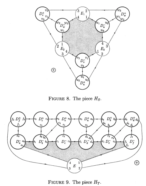
Let $H_{S}$ and $H_{T}$ be the pieces of a punctured Heegaard diagram shown in Figure 8

and 9, respectively. These pieces correspond to either (trice-punctured sphere) $\cross S^{1}$ and

(once-punctured torus) $\cross S^{1}$, respectively. Again, we consider that the curves $\alpha$

are

bold

and the

curves

$\beta$

are

thin in the figure.

FIGURE 8. The piece $H_{S}$.

FIGURE 9. The piece $H_{T}$.

Let $g$ be a non-negative integer and $b$ be an integer. Let $(p_{1}, q_{1}),$ $(p_{2}, q_{2}),$ _$\ldots,$$(p_{r}, q_{r})$ be

Assume that $g+r\geq 2$. Prepare $g+r-1$ copies $H_{s}^{1},$$H_{s}^{2},$

$\ldots,$$H_{s}^{g+r-2}$ of the piece $H_{S}$

and $g$ copies $H_{T}^{1},$$H_{T}^{2},$ $\ldots,$$H_{T}^{g}$ ofthe piece $H_{T}$. First, attach the boundary

$E$of the piece

$H_{b}$ of punctured Heegaard diagram to the boundary $\partial E_{1}$ of the piece $H_{S}^{1}$ so that the

numbers 1, 2, 3, 4 on the both boundary circles match. For odd $k$ with $1\leq k\leq r$, attach

the boundary $I$ ofthe piece $H_{(p_{k},q_{k})}$ ofpiece to the boundary $\partial E_{2}$ of the piece $H_{S}^{k}$ in the

same manner as above. For even $k$ with $1\leq k\leq r$, attach the boundary $E$ of the piece

$H_{(p_{k},p_{k}-q_{k})}$ of

a

punctured Heegaard diagram to the boundary $\partial E_{2}$ of the piece $H_{S}^{k}$ in the

same

manner

as

above. For $1\leq k\leq g-1$, attach the boundary $E$ of the piece $H_{T}^{k}$ to the

boundary $\partial E_{2}$ of the piece $H_{s}^{r+k}$ in the

same manner as

above. Attach the boundary $E$

of the piece $H_{T}^{g}$ to the boundary $\partial E_{3}$ of the piece $H_{s}^{g+r-1}$ in the

same

manner as

above.

Note that

now we

have $g+r-1$ components ofpieces $W_{1},$ $W_{2},$

$\ldots,$$W_{g+r-1}$ ofapunctured

Heegaard diagram such that

$\bullet$ $W_{1}$ contains both $H_{b}$ and $H_{s}^{1}$; $\bullet$ $W_{k}$ contains $H_{S}^{k}$ for $2\leq k\leq r$;

$\bullet$ $W_{k}$ contains $H_{T}^{k}$ for $r<k\leq g+r-2$; and $\bullet$ $W_{g+r-1}$ contains both $H_{T}^{g+r-1}$ and $H_{T}^{g+r}$.

For each even $k$ with $1\leq k\leq g+r-2$, change the fixed normal direction ofthe diagram

$W_{k}$ and

Now

we

get

a

punctured Heegaard diagram by attaching the boundary $\partial E_{3}$ of the

diagram $W_{k}$ to the boundary $\partial E_{1}$ of the diagram _{$W_{k+1}$} for $1\leq k\leq g+r-2$. We denote

it by $H_{(g;b;(p_{1},q_{1}),(p_{2},q_{2}),\ldots,(p,,q,))}$.

If $g+r\leq 2$, attach the piece $H_{b}$ of a punctured diagram to the boundary $\partial E_{1}$ of the

piece $H_{S}^{1}$. Moreover, attach the rest ofthe pieces $H_{(p_{i},q_{i})}$ and copies of $H_{T}$, if any, to the

boundaries $E_{2}$ and $E_{3}$. In particular, if $g+r<2$, attach the copies of $H_{C}$ to all the

remaining boundary components of $H_{s}^{1}$.

Theorem 2.1. The punctured Heegaard diagmm $H_{(g;b;(p_{1},q_{1}),(p_{2},q_{2}),\ldots,(p_{r},q_{f}))}$ corresponds to

the

_{Seifert fibered}

_3-manifold

$S(g;b;(p_{1}, q_{1}), (p_{2}, q_{2}), \ldots, (p_{r}, q_{r}))$ with a standard $Spin^{c}$

structure.

Pmof.

The idea ofthe proof isto construct the pieces ofthepunctured Heegaarddiagram

corresponding to the pieces of the DS-diagram constructed in [11] following the proof of Theorem 5.5.

Let $\pi,$ $B,$ $W$ and $e$ be

as

described in Section 1.6. Set $A:=\eta(e;\partial\eta(P))$. Recall that $e$

has the $B$ part

on

one side and the $W$

one on

the other side. The key idea is to draw

a

simple closed curve $C$ in $A$ such that

(1) $C$ is isotopic to $e$ in $A$;

(2) $C\cap e\neq\emptyset$ and $C$ intersects $e$ transversely; and

(3) $C\cap\pi^{-1}(S(P))\subset e\backslash \pi^{-1}(V(P))$.

Let $\mathcal{H}_{L}$ beapieceofDS-diagram (onthe annulus) showninFigure 10 (i). Thisdiagram

was

constructed in [11]. The curve $e$ lies horizontally in the middle part of the diagram

and it separates the diagram into B-part, on the upper side, and W-part, on the lower

side. Then the intersection $C\cap \mathcal{H}_{R}$is depicted bythe bold linesin Figure 10 (ii). The two

curves $C\cap \mathcal{H}_{R}$cut the annulus intotwodisks, the under pieceof which correspondsto the

joining disk. Note that the disk $D^{-}$ shown in the figure is identified via the projection $\pi$

3 2

く i

$(\mathfrak{i})$ $\{\dot{t}i)$ $(\mathfrak{i}ii)$

FIGURE 10. From $\mathcal{H}\iota$ to $H_{L}$

.

$\oplus$

FIGURE 11. The pie く ce $H_{L}$ ofapunctured Heegaard diagram.

For the other pieces shown in [11],

we

can

apply the

same

argument. Cnsequently, $weD$

get the assertion.

Remark2.2. Forgetting thejoiningdiskofthediagram $II_{(g;b;(p_{1},q\iota)_{)}\infty,\varphi),\ldots,(p_{r},q,))}$,

one

has

a

Heegaard diagram of theSeifert fibered manifold$S(g;b, (p_{1}, q_{1}), (p_{2}, q_{2}), \ldots, (p_{r}, q_{r}))$

.

For

es&

pieceoftheHeegaard diagram corresponding to

a

singularfiberobtained in the above

construction, thediagram

can

bedestabilized

so

thatit is

a

diagramon aonce-punctured

torus.

2.2. Algorithm. Let $M$bea Seifert fibered 3-manifold$S(g;b;(p_{1}, q_{1}),$$(p_{2}, q_{2}),$

$\ldots$ ,$(p_{r}, q_{r})$

.

Let $fI_{\text{く}S(g;b;\phi,q_{1}),\infty,\alpha),.,.,\phi_{Y},q_{r}))}=(S_{g};\alpha, \beta, D)$ be the punctured Heegaard diagram

con-structed

as above.

Recall that

once

given

a

punctured Heegaard diagram, the Heegaard

surface$S_{9}$ assumed tobenaturallyoriented

as

explainedin Section1. Let $F$ be afield and $\varphi:\mathbb{Z}[H_{1}$く$M_{(S_{1}\alpha,\beta;D)})]arrow F$ be

a

ring homomorphism. We

can

calculate the

Reidemeister-Turaev torsion of the standard Spin’ structure of $M$, i.e. the principal Reidemeister

torsion $7^{\tau\varphi}(M)$, in the following algorithmic way (cf. [7]):

Step 1: Orient a and $\beta$, and take base points of$\beta$ following the rule prescribed in

Section 1.

Step 2: Get apresentation $\langle x_{\lambda},$

$\ldots$,$x_{g}|r_{1},$ $\ldots,$

$r_{g}\rangle$ of $\pi_{1}(M, *)$ using the punctured Heegaard diagram $(S;\alpha,\beta_{2}\cdot D)$

as

inthe rule of Section 1.5.

Step 3: Find

an

arbitrarydualsystem $\gamma$ of$\beta$ in the diagram $(S;\alpha, \beta;D)$ and relate

Step 4: Ifthereexist twointegers $k,$$l\in\{1, \ldots, g\}$such that all of$\det B_{k,l},$ $\varphi([y_{l}])-1$

and $\varphi([y_{l}])-1$ are nonzero, then wehave

$\tau^{\varphi}(M, \mathcal{V}_{st})=\pm\frac{\det B_{k,l}}{(\varphi([x_{k}])-1)(\varphi([y_{l}])-1)}\in F^{\cross}/\pm 1$ ,

where $B_{k,l}$ is the $(k, l)$-minor of the matrix $( \varphi([\frac{\partial r_{j}}{\partial x_{i}}]))_{1<i,j\leq g}$. If there are not

such integers $k$ and $l$, then it turns out that the twisted chain complex $C^{\varphi}(M)$ is

not acyclic, hence we have $\tau^{\varphi}(M, V_{st})=0$ by definition.

Remark that due to [8] and [14], the above alsogives

an

purely combinatorial algorithm

to compute the Seiberg-Witten invariant of standard $Spin^{c}$ structure when the given

Seifert fibered 3-manifold has the first homology group of infinite order. 3. EXAMPLES AND OBSERVATIONS

3.1. Lens spaces. Using the algorithm in Section 2.2 for a lens space $L(p, q)$_, we get a

Spi$n^{}$ structure on $L(p, q)$ and a presentation of $\pi_{1}(L(p, q))$ corresponding to the $Spin^{c}$ structure can be written

as

$\pi_{1}(L(p, q))=\langle x|x^{p}\rangle$ after simplifying the generators and

relators. Then for a representation $\varphi$ : $H_{1}(L(p, q))arrow F^{\cross}$, we have a well-known result

$\tau^{\varphi}(L(p, q), [V_{st}])=\pm 1/(\zeta-1)(\zeta^{r}-1)$, where $\zeta=\varphi([x])$.

Let

us

focus

on

the lens space$L(11,1)$

.

Thesetof the values of the Reidemeister-Turaev

torsions ofthe Spi$n^{}$ structures of $L(11,1)$ is:

$\{\tau^{\varphi}(L(11,1), [\mathcal{V}])|[\mathcal{V}]\in Spin^{c}(L(11,1))\}=\{\pm\frac{(^{i}}{(\zeta-1)^{2}}\in F^{\cross}/\pm 1$ $0\leq i<11\}$ . In this set, only the two values $\pm 1/(\zeta-1)^{2}$ and $\pm\zeta^{2}/(\zeta-1)^{2}$ can be modified so that the

numerator is $\pm 1$ and the denominator are the form of $(\zeta^{a}-1)(\zeta^{b}-1)$ for some $a,$$b\in \mathbb{Z}$.

In fact, we have $\pm\zeta^{2}/(\zeta-1)^{2}=\pm 1/(\zeta^{10}-1)^{2}$. Note that the value $\pm 1/((-1)^{2}$ is the

torsionof the Spi$n^{}$ structurederived from thestandard Seifert fibration of $(L(11,1))$ and

$\pm\zeta^{2}/(\zeta-1)^{2}$ is that ofthe Spi$n^{}$ structure derived from the standard Seifert fibration of

$(L(11,10))$. $(^{6}/(\zeta-1)^{2}$ $\zeta^{5}/(\zeta-1)^{2}$ $\zeta^{7}/((-1)^{2}\cdot$ $\zeta^{8}/(\zeta-1)^{2}$

.

$\zeta^{9}/(\zeta-1)^{2}$

.

$\zeta^{10}/(\zeta-1)^{2}$

.

$1/(\zeta-1)^{2}0$ $\zeta^{4}/(\zeta-1)^{l}$ $\zeta^{3}/(\zeta-1)^{2}$ $o(^{2}/(\zeta-1)^{2}=1/(\zeta^{10}-1)^{2}$ $\zeta/(\zeta-1)^{2}$

FIGURE 12. The set ofSpi$n^{}$ structureson $L(11,1)$ and their Reidemeister-Turaev torsions (the signs $\pm$

are

omitted). The white dots

are

the standard

Spi$n^{}$ structures.

Next, consider the lens space $L(11,2)$. For this manifold, the set of the values of the

$\{\tau^{\varphi}(L(11,2), [\mathcal{V}])|[V]\in Spin^{c}(L(11,2))\}=\{\pm\frac{\zeta^{i}}{(\zeta-1)(\zeta^{6}-1)}\in F^{\cross}/\pm 1$ _{$0\leq i<11\}$}

In this set, exactly the four values $\pm 1/(\zeta-1)(\zeta^{6}-1),$ $\pm\zeta/(\zeta-1)(\zeta^{6}-1),$ $\pm(^{6}/(\zeta-$

$1)(\zeta^{6}-1)$ and $\pm\zeta^{7}/(\zeta-1)(\zeta^{6}-1)$ can be modified so that the numerator is $\pm 1$ and

the denominator are the form of $(\zeta^{a}-1)(\zeta^{b}-1)$ for some $a,$$b\in \mathbb{Z}$. In fact, we have

$\pm\zeta/(\zeta-1)(\zeta^{6}-1)=\pm 1/(\zeta^{6}-1)(\zeta^{10}-1),$ $\pm\zeta^{6}/(\zeta-1)(\zeta^{6}-1)=\pm 1/(\zeta-1)(\zeta^{5}-1)$ and

$\pm\zeta^{7}/(\zeta-I)(\zeta^{6}-1)=\pm 1/(\zeta^{5}-1)(\zeta^{10}-1)$.

$\zeta^{0}/(\zeta-1)(\zeta^{6}-1)=1/(\zeta-1)(\zeta’\sigma-1)0$ $\zeta^{6}/(\zeta-1)(_{\backslash }^{\Gamma 6}-1)$

$\zeta^{-}/(\zeta-1)(\zeta^{6}-1)=1/(\zeta^{10}-l)(\zeta^{5}-1)0$ $\zeta^{4}/(\zeta-1)(\zeta^{6}-1)$

$\zeta^{8}/(\zeta-1)(\zeta^{6}-1)$

.

$\zeta^{3}/(\zeta-1)(\zeta^{6}-1)$ $\zeta^{9}/(\zeta-1)(\sigma^{6}-1)$

.

$\zeta^{2}/(\zeta-1)(\zeta^{6}-1)$

$\zeta^{10}/(\zeta-1)(\zeta^{6}-1)$

.

$\circ(/(\zeta-1)(C^{6}-1)=1/(\zeta^{10}-1)(\overline{t}^{6}-1)$ $1/(\zeta-1)(\zeta^{6}-1)0$

FIGURE 13. Theset ofSpi$n^{}$ structures on$L(11,2)$ and their Reidemeister-Turaev torsions (the signs $\pm$ are omitted). The white dots are the standard

Spi$n^{}$ structures.

Observation 3.1. The Reidemeister- Tumev torsion

_of

a Spi$n^{}$ structure

of

a lens space

is

_of

the$fom\pm 1/(\zeta^{a}-1)(\zeta^{b}-1)$

for

some $a,$ $b\in \mathbb{Z}$

if

and only

if

the Spi$n^{}$ structure is standard.

3.2. $S_{g}\cross S^{1}$

.

Let $S_{g}$ be a closed orientable surface of genus $g>1$ and consider the Seifert

fibered 3-manifold $S_{g}\cross S^{1}$. Using the algorithm in Section 2.2 for $S_{g}\cross S^{1}$, we get a $Spin^{c}$

structure $V_{st}$ on $S_{g}\cross S^{1}$ and a presentation of $\pi_{1}(S_{g}\cross S^{1})$ corresponding to the $Spin^{c}$

structure can be written as

$\pi_{1}(S_{g}\cross S^{1})=\langle x_{1},$$x_{2},$ _{$\ldots,$ $x_{2g},$}$y|x_{i}yx_{i}^{-1}y^{-1},$$i=1,2,$

$\ldots,$$2g,$$\prod_{i=1}^{g}(x_{2i-1}x_{2i}x_{2i-1^{-1}}x_{2i^{-1}})\rangle$,

and its abelianization is:

$H_{1}(S_{g} \cross S^{1}):=(\bigoplus_{i=1}^{2g}\mathbb{Z}\langle[x_{i}]\rangle)\oplus \mathbb{Z}\langle[y]\rangle$.

Let $\varphi:\mathbb{Z}[H_{1}(S_{g}\cross S^{1};\mathbb{Z})]arrow F$be aring homomorphism to a field $F$ such that each of

$\zeta_{i}=\varphi([x_{i}])$ and $\zeta=\varphi([y])$ has an infinite order. Then we have

The set of the values of the Reidemeister-Turaev torsions of the Spi$n^{}$ structures of

$S_{g}\cross S^{1}$ is:

$\{\tau^{\varphi}(S_{g}\cross S^{1}, [V])|[V]\in Spin^{c}(S_{g}\cross S^{1})\}$

$=$ $\{\pm\zeta_{1}^{i_{1}}\cdots\zeta_{2g}^{i_{2g}}\zeta^{i}(\zeta-1)^{2g-2}\in F^{\cross}/\pm 1|i_{1},$

$\ldots,$$i_{2g},$ $i\in \mathbb{Z}\}$

...

$\bullet$ $\bullet$

$\bullet\zeta^{-1}(\zeta-1)^{\underline{?}_{g-2}}$

:

_: $:$ :

:

:

...

$\bullet\bullet\bullet$ $\zeta(\zeta-1)^{2g-2}$ $\bullet\bullet$

...

...

$\bullet$ $\bullet$ $o(\zeta-1)^{2g-2}$ $\bullet$ $\bullet$

.. .

$\bullet$ $\bullet$

...

$:$ :

:

: : :

...

$\bullet$ $\bullet$ $\bullet(\zeta-1)^{g-1}(\zeta^{-1}-1)^{g-1}$ $\bullet$ $\bullet$

$arrow a$ Spi$n^{}$ structure derivedfromaSpin structure

:

:

_.

:

_:

:

_.

:

...

$\bullet$ $\bullet$ $\bullet$ $\bullet$ $\bullet$

...

$\bullet$ $\bullet$ $o\zeta^{-(2g-2)}(\zeta-1)^{2g-2}=(\zeta^{-1}-1)^{2g-2}$

...

$\bullet$ $\bullet$ $\bullet$ $\bullet$ $\bullet$

...

: : :

:.

:

:

FIGURE 14. The set ofSpi$n^{}$ structures on $S_{g}\cross S^{1}$ and their Reidemeister-Turaev torsions (the signs $\pm$

are

omitted). The white dots

are

the standard

Spi$n^{}$ structures.

Observation 3.2. The Reidemeister- Tumev torsion

_of

a Spi$n^{}$ structure

of

$S_{g}\cross S^{1}$ is

of

the$fom\pm(\zeta^{a}-1)^{2g-2}$

for

some

$a\in \mathbb{Z}$

if

and only

if

the Spi$n^{}$ structure is standard. 3.3. Brieskorn 3-manifolds. The Brieskom manifold $\Sigma(p, q, r)$ of type $(p,q, r)$ is a

closed 3-manifold defined by:

$\Sigma(p, q, r):=\{(x, y, z)\in \mathbb{C}^{3}||x|^{2}+|y|^{2}+|z|^{2}=1, x^{p}+y^{q}+z^{r}=0\}$,

where$p,$$q$ and $r$ are integers greater than 1.

$\Sigma(p, q, r)$ is the r-fold branchedcovering ofthe 3-sphere$S^{3}$ branched alonga torusknot

or link oftype $(p, q)$. The first integral homology groups of the Brieskom manifolds is

$H_{1}(\Sigma(p, q, r);\mathbb{Z})=\{\begin{array}{ll}1 n=\pm 1(mod 6)\mathbb{Z}/3\mathbb{Z} n=\pm 2(mod 6)\mathbb{Z}2\mathbb{Z}\oplus \mathbb{Z}/2\mathbb{Z} n=3(mod 6)\mathbb{Z}\oplus \mathbb{Z} n=0(mod 6)\end{array}$

Usingthe algorithm inSection2.2for $\Sigma(2,3,6n)$, wegetaSpi$n^{}$ structure$V_{st}$ on$\Sigma(2,3,6n)$

as

$\pi_{1}(\Sigma(2,3,6n))=\langle x_{1},$$x_{2},$

$\ldots,$$x_{6n}|x_{i}x_{i+6n-1^{-1}}x_{i+1^{-1}},1\leq i\leq 6n\rangle$

and its abelianization is:

$H_{1}(\Sigma(2,3,6n);\mathbb{Z})$ $:=\mathbb{Z}\langle[x_{1}]\rangle\oplus \mathbb{Z}\langle[x_{2}]\rangle$

.

Let $\varphi$: $\mathbb{Z}[H_{1}(\Sigma(2,3,6n);\mathbb{Z})]arrow F$ be a ringhomomorphism to a field $F$ such that each of

$\zeta_{1}=\varphi([x_{1}])$ and $\zeta_{2}=\varphi([x_{2}])$ has an infinite order. Then we have

$\tau^{\varphi}(\Sigma(2,3,6n), [V_{st}])=\pm\frac{\det(\varphi([\frac{\partial x_{i}x_{i+6n-1^{-1-1}}x_{i+1}}{\partial x_{j}}]))_{1,1}}{(\zeta_{1}^{-1}-1)(\zeta_{1}-1)}=\pm n$

.

Theset ofthe values ofthe Reidemeister-Turaevtorsions of the Spi$n^{}$ structuresof$S_{g}\cross S^{1}$

is:

$\{\tau^{\varphi}(\Sigma(2,3,6n), [\mathcal{V}])|[\mathcal{V}]\in Spin^{c}(\Sigma(2,3,6n))\}=\{\pm n(_{1}^{i_{1}}\zeta_{2}^{i_{2}}\in F^{\cross}/\pm 1|i_{1},$$i_{2}\in \mathbb{Z}\}$

.

.

_.

_.

.

.

.

...

$n\zeta_{1}^{-2}\zeta_{2}^{2}$ $n\zeta_{1}^{-1}\zeta_{2}^{2}$ $n\zeta_{2}^{2}$ $n\zeta_{1}\zeta_{2}^{2}$

’

$n\zeta_{1}^{2}\zeta_{2}^{2}$

..

.

...

$n\zeta_{1}^{-2}\zeta_{2}$ $n\zeta_{1}^{-1}\zeta_{2}$ $n\zeta_{2}$ $n\zeta_{1}\zeta_{2}$’ $n\zeta_{1}^{2}\zeta_{2}$

...

.

. .

$n\zeta_{1}^{-2}$ $n\zeta_{1}^{-1}$ _$n$ $n\zeta_{1}$ $n\zeta_{1}^{2}$

$0arrow_{aSpiri^{c}}$

struct$\iota irederii\cdot edf_{I}om$aSpin structurc

.

.

. $n\zeta_{1}^{-2}\zeta_{2}^{-1}$ _$il$$\zeta_{1}^{-1}(_{2}^{-1}$ $n\zeta_{2}^{-1}$ $n(\iota\zeta_{2}^{-1}$ $n\zeta_{1}^{2}\zeta_{2}^{-1}$

.

. .

. . .

$n\zeta_{1}^{-2}\zeta_{2}^{-2}$ $n\zeta_{1}^{-1}\zeta_{2}^{-2}$ $n\zeta_{2}^{-2}$ $n\zeta_{1}\zeta_{2}^{-2}$ $n\zeta_{1}^{2}\zeta_{2}^{-2}$

. .

.

:

:

:

_.

:

_.

.

FIGURE 15. The set of $Spin^{c}$ structures on $\Sigma(2,3,6n)$ and their

Reidemeister-Turaev torsions (the signs $\pm$ are omitted). The white dot

is the standard Spi$n^{}$ structure.

Observation 3.3. The Reidemeister- Tumev torsion

_of

a Spi$n^{}$ structure

of

the Brieskom

3-manifolds

$\Sigma(2,3,6n)(n\in \mathbb{N})$ is

of

the $form\pm a$

for

some $a\in \mathbb{Z}$

if

and only

if

the $Spin^{c}$ structure is standard.

From the aboveobservations, wemayroughlysay that the Reidemeister-Turaev torsions of the standardSpi$n^{}$ structures of a Seifert fibered 3-manifoldhave standardvaluesamong the set ofthe Reidemeister-Turaev torsions of all Spi$n^{}$ structures on the manifold.

Acknowledgements. The author is supported by Grant-in-Aid forYoung Scientists (B)

REFERENCES

[1] G. Amendola, R. Benedetti, F. Costantino, C. Petronio, Branched spines _{of 3-manifolds} and

torsion _ofEulerstructures, Rend. Ist. Mat. Univ. TYieste 32 (2001), 1-33.

[2] R. Benedetti, C. Petronio, Bmnched Standard Spines _of3-manifolds, Lecture Notes in Math.

1653, Springer-Verlag, Berlin-Heiderberg-New York, 1997.

[3] R. Benedetti, C. Petronio, Reidemeister-hmev torsion _of3-dimensional Euler structures with

simple boundary tangency and$pseudo-Legend\dot{m}an$ knots, Manuscripta Math. 106 (2001), 13-74.

[4] W. Floyd, U.Oertel, Incompressible_surfacesviabmnchedsurfaces, Topology23 (1984), 117-125.

[5] A. Fomenko, S. Matveev, Algorithmic and Computer Methods_for Three-Manifolds, Mathematics

and its Applications425, Kluwer Academic Publishers, Dordrecht, 1997.

[6] Y. Koda, Spines, Heegaard splittings and the Reidemeaster-Turaev torsion _of Euler structure,

Tokyo J. Math. 30 (2007), 417-439.

[7] Y. Koda, A Heegaard-type presentation _ofbmnched spines and the Reidemeister-Tumev torsion,

Math. Z. 260 (2008), 203-228.

[8] G. Mengand C. H. Taubes, $\underline{SW}=$ Milnortorsion, Math. Res. Lett. 3 (1996), 137-147.

[9] L. I. Nicolaescu, The Reidemeister Torsion _of 3-Manifolds, de Gruyter Stud. Math. 30, de

Gruyter, Berlin, 2003.

[10] U. Oertel, Incompressible bmnchedsurfaces, Invent. Math. 76 (1984), 385-410.

[11] T. Taniguchi, K. Tsuboi, M. Yamashita, Systematic singular triangulations for all Seifert

mani-folds, TokyoJ. Math. 28 (2005), 539-561.

[12] V. Turaev, Euler $str\tau\iota cture$, nonsingular vector flows, and Reidemeister-type torsions, Math.

USSR-Izv. 34 (1990), 627-662.

[13] V. Turaev, Torsion invariants _of Spi$n^{}$ -structures on 3-manifolds, Math. Res. Lett. 4 (1997),

679-695.

[14] V. Turaev, A combinatorial_{fomulation for}the Seiberg-Witten invariants _of3-manifolds, Math.

Res. Lett. 5 (1998), 583-598.

[15] V. Turaev, Introduction to combinatorial torsions, Lectures in Mathematics ETH Z\"urich,

Birkh\"auserVerlag, Basel-Boston-Berlin, 2001.

[16] V. Turaev, Surgery _{fomula for} torsions and Seiberg-Witten invariants _of 3-manifolds,

$arXiv:math.GT/0101108$.

$[17|$ V. Turaev, Torsions

of

3-dimensional Manifolds, Progress in Math. 208, Birkh\"auser Verlag,

Basel-Boston-Berlin, 2002.

MATHEMATICAL INSTITUTE, TOHOKU UNIVERSITY, SENDAI, 980-8578, JAPAN