On numerical methods for analysis of
chaotic phenomena
in
free boundary problems
Hitoshi IMAI
(
今井 仁司
)
and Toshiki
TAKEUCHI
(竹内
敏己
)
Department
of Applied Physics and
Mathematics,
Faculty
of Engineering,
University
of
Tokushima,
Tokushima 770-8506, Japan.
(
徳島大学 工学部
)
1Introduction
The free boundary problems
are
very
important,
because they
often
arise
from the
practical
situations. They
are
nonlinear,
so
they easily involve chaotic phenomena. Thus investigation
of chaotic phenomena in
free
boundary problems is
very
important.
The investigation is carried out via analysis
of bifurcation and
attractors[18].
In the
pre-vious work
bifurcation
phenomena in afree boundary problem
related
to natural
convection
were
analyzed numerically[20].
Attractors
in
free
boundary problems
were
analyzed
the0-retically.
Attractors
or
inertial
sets
for
the phase
field
model
were
analyzed in [3],
$[8]-[14]$
.
Attractors for the problem in which the motion
of
the
free
boundary is given explicitly
were
analyzed in [1].
However,
in
these
papers concrete
analysis
of attractors
was
not
carried
out,
because their analysis
was
based
on
PDE systems.
Attractors of
the
ODE
system play
avery
important
role. This is because they
are
useful
for concrete analysis[5, 6, 15].
For
autonomous
ODE
systems
numerical
computation
of Lyapunov exponents is easily
carried
out.
If
there
exist
positive Lyapunov exponents,
chaotic phenomena exist. However, it is
difficult
to
derive the autonomous
ODE
system
which approximates the
PDE
system describing
afree
boundary problem.
In the
paper amethod for numerical
computation
of attractors
in
free
boundary problems
and Lyapunov exponents is presented. To
see
the procedure
of
the
method
afree boundary
problem
with
some
parameters
is
considered. It
is
of
the type
of
atw0-phase
Stefan
problem.
The
method consists
of
SCM(Spectral
Collocation
Method)
[4],
the fixed
domain method[ll]
and
transformation from
the
nonautonomous
system
into the
autonomous
one[2].
2Test
problem
We consider the following
one-dimensional
free boundary problem with
some
parameters
数理解析研究所講究録 1210 巻 2001 年 115-128
Problem
1. For
parameters
lcr”l
$|_{\ovalbox{\tt\small REJECT}}\mathrm{d}1|s_{0}|<1,0\ovalbox{\tt\small REJECT}$r
$\ovalbox{\tt\small REJECT}$1,
q
$\mathrm{a}\mathrm{n}\mathrm{d},\ovalbox{\tt\small REJECT}^{-\mathrm{b}}$
,
find
$\mathrm{u}"(_{\ovalbox{\tt\small REJECT}}\mathrm{z},$
t)
and
$\ovalbox{\tt\small REJECT}(t)$such that
$u_{t}^{+}(x, t)=u_{xx}^{+}(x, t)+g^{+}(x, t)$
,
$0<t$
,
$-1<x<s(t)$
,
(2.1)
$u^{+}(-1, t)=h^{+}(t)$
,
$0\leq t$
,
(2.2)
$u^{+}(s(t), t)=0$
,
$0\leq t$
,
(2.3)
$u^{+}(x, 0)=f^{+}(x)$
,
$-1<x<s_{0}$
,
(2.4)
$u_{t}^{-}(x, t)=u_{xx}^{-}(x, t)+g^{-}(x, t)$
,
$0<t$
,
$s(t)<x<1$
,
(2.5)
$u^{-}(1, t)=h^{-}(t)$
,
$0\leq t$
,
(2.6)
$u^{-}(s(t), t)=0$
,
$0\leq t$
,
(2.7)
$u^{-}(x, 0)=f^{-}(x)$
,
$s_{0}<x<1$
,
(2.3)
$\frac{d}{dt}s(t)=-k^{+}(t)u_{x}^{+}(s(t), t)+k^{-}(t)u_{x}^{-}(s(t), t)$
,
$0<t$
,
(2.9)
$s(0)=s_{0}$
(2.10)
where
$k^{\pm}(t)=r+(1-r) \frac{1}{2}\frac{1\pm\beta\sin t}{\pm 1+\alpha^{\pm}\sin t}\beta\cos t$
,
(2. 1)
$h^{\pm}(t)=\pm 1+\alpha^{\pm}\sin(\omega^{\pm}t)$,
(2.12)
$g^{\pm}(x, t)=q( \pm\frac{(\beta-\alpha^{\pm})\cos t}{(1\pm\beta\sin t)^{2}}(x-\beta \mathrm{s}.\mathrm{n}t)\pm\frac{\pm 1+\alpha^{\pm}\sin t}{1\pm\beta\sin t}\beta\cos t)$
,
(2.1 )
$f^{+}(x)=(x-s_{0})(a(x+1)- \frac{1}{s_{0}+1})$
,
(2.14)
$f^{-}(x)$
$=(x-s_{0})(b(x-1)+ \frac{1}{s_{0}-1})$
.
(2.15)
Parameters
$a$,
$b$should be
determined such that
$f^{+}(x)\geq 0$
,
$f^{-}(x)$
$\leq 0$.
Remark 1.
For
a
$=b=s_{0}=r=0$
,
$\omega^{\pm}=1$and q
$=1$
,
there
are
exact
solutions
as
follows:
$s(t)=s_{p}(t)\equiv\beta\sin t$
,
(2.16)
$u^{\pm}(x, t)= \frac{\mp h^{\pm}(t)}{1\pm s_{p}(t)}(x-s_{p}(t))=\mp\frac{\pm 1+\alpha^{\pm}\sin t}{1\pm\beta\sin t}(x-\beta\sin t)$
.
(2.1 )
3Our
method
In this section amethod for derivation of the
ODE
system
which
approximates the PDE
system
describing
afree
boundary problem
is
presented.
It consists of the fixed
domai
$\mathrm{n}$116
method and
SCM.
For numerical
computation
of
Lyapunov exponents
transformation from
the
nonautonomous
system
into
the autonomous
one
is also
necessary.
To
see
the
procedure
the
method
is
applied
to
Problem 1.
3.1
Spectral
collocation method
The spectral
methods
are
superior
in accuracy[4]. In
particular,
the application of
SCM
is
similar
to
that
of FDM.
So,
it is
easily
applied to
nonlinear
problems.
In the paper,
SCM
using Chebyshev Polynomials
and Chebyshev-Gauss-Lobatto case’s collocation
points
are
used. In
SCM
it is easy
to
increase
the order of the
approximation by increasing
the
number
of collocation
points.
This feature is
quite
remarkable and different from other discretization
methods.
3.2
Fixed
domain method
SCM
can
not
be
applied directly
to
afree
boundary problem
due
to
the
unknown
shape
of the domain. To avoid this difficulty,
we
use
the
fixed
domain method
$[7, 11]$
.
Mapping
functions
are
introduced
for
mapping the
unknown domain
to
the fixed
rectangular
domain.
We
use
the following mapping
function
(variable transformation) :
$(x, t)arrow(\xi,\tilde{t})$such
that
$t=t(\tilde{t})=\tilde{t}$
,
$0\leq t$
,
(3.18)
$x=x(\xi,\tilde{t})=\{$
$\frac{\tilde{s}(\tilde{t})+1}{2}(\xi+1)-1$
,
$0\leq t$
,
$-1\leq x\leq s(t)$
,
$\frac{1-\tilde{s}(\tilde{t})}{2}(\xi-1)+1$,
$0\leq t$
,
$s(t)\leq x\leq 1$
.
(3.19)
Using
these mapping functions,
we
define
$\tilde{s}(\tilde{t})=s(t(\tilde{t}))$
,
(3.20)
$\tilde{u}^{+}(\xi,\tilde{t})=u^{+}(x(\xi,\tilde{t}),$$t(\overline{t}))$
,
(3.21)
$\tilde{u}^{-}(\xi,\tilde{t})=u^{-}(x(\xi,\tilde{t}),$$t(\tilde{t}))$
.
(3.22)
Then,
Problem
1is
transformed
into the
following fixed
boundary problem.
Problem 2. Find
$\tilde{u}^{\pm}(\xi,\tilde{t})$and
$\tilde{s}(\tilde{t})$such that
$\tilde{u}_{\tilde{t}}^{+}(\xi,\tilde{t})=-k^{+}(\tilde{t})\frac{2(\xi+1)}{(\tilde{s}(\tilde{t})+1)^{2}}\tilde{u}_{\xi}^{+}(1,\tilde{t})\tilde{u}_{\xi}^{+}(\xi,\tilde{t})$ $-k^{-}( \tilde{t})\frac{2(\xi+1)}{\tilde{s}(\tilde{t})^{2}-1}\tilde{u}_{\xi}^{-}(-1,\tilde{t})\tilde{u}_{\xi}^{+}(\xi,\tilde{t})+\frac{4}{(\tilde{s}(\tilde{t})+1)^{2}}\tilde{u}_{\xi\xi}^{+}(\xi,\tilde{t})$ $+q \{\frac{(\beta-\alpha^{+})\cos\tilde{t}}{(1+\beta\sin\tilde{t})^{2}}(\frac{\tilde{s}(\tilde{t})+1}{2}(\xi+1)-1-\beta\sin\tilde{t})$ $+ \frac{(1+\alpha^{+}\sin\tilde{t})\beta\cos\tilde{t}}{1+\beta\sin\tilde{t}}\}$,
$0<\tilde{t}$,
$-1<\xi<1$
,
(3.24)
$\tilde{u}^{+}(-1,\tilde{t})=1+\alpha^{+}\sin(\omega^{+}\tilde{t})$,
$0\leq\tilde{t}$,
(3.24)
$\tilde{u}^{+}(1,\tilde{t})=0$,
$0\leq\tilde{t}$,
(3.25)
$\tilde{u}^{+}(\xi, 0)=\frac{1}{4}(\xi-1)\{a(s_{0}+1)^{2}(\xi+1)-2\}$
,
$-1<\xi<1$
,
(3.24)
$\tilde{u}_{\overline{t}}^{-}(\xi,\tilde{t})=-k^{+}(\tilde{t})\frac{2(\xi-1)}{\tilde{s}(\tilde{t})^{2}-1}\tilde{u}_{\xi}^{+}(1,\tilde{t})\tilde{u}_{\xi}^{-}(\xi,\tilde{t})$$-k^{-}(t)$
$\frac{2(\xi-1)}{(\tilde{s}(t)-1)^{2}}\tilde{u}_{\xi}^{-}(-1,\tilde{t})\tilde{u}_{\xi}^{-}(\xi,\tilde{t})+\frac{4}{(\tilde{s}(\tilde{t})-1)^{2}}\tilde{u}_{\xi\xi}^{-}(\xi,\tilde{t})$ $+q \{-\frac{(\beta-\alpha^{-})\cos\tilde{t}}{(1-\beta\sin\tilde{t})^{2}}(\frac{1-\tilde{s}(\tilde{t})}{2}(\xi-1)+1-\beta\sin\tilde{t})$ $+ \frac{(1-\alpha^{-}\sin\tilde{t})\beta\cos\tilde{t}}{1-\beta\sin\tilde{t}}\}$,
$0<\tilde{t}$,
$-1<\xi<1$ ,
(3.27)
$\tilde{u}^{-}(-1,\tilde{t})=0$,
$0\leq\tilde{t}$,
(3.28)
$\tilde{u}^{-}(1,\tilde{t})=-1+\alpha^{-}\sin(\omega^{-}\tilde{t})$,
$0\leq\tilde{t}$,
(3.29)
$\tilde{u}^{-}(\xi, 0)=\frac{1}{4}(\xi+1)\{b(s_{0}-1)^{2}(\xi-1)-2\}$
,
$-1<\xi<1$
,
(3.30)
$\frac{d}{d\tilde{t}}\tilde{s}(\tilde{t})=-k^{+}(\tilde{t})\frac{2}{\tilde{s}(\tilde{t})+1}\tilde{u}_{\xi}^{+}(1,\tilde{t})-k^{-}(\tilde{t})\frac{2}{\tilde{s}(\tilde{t})-1}\tilde{u}_{\xi}^{-}(-1,\tilde{t})$
,
$0<\tilde{t}$,
(3.31)
$\tilde{s}(0)=s_{0}$
.
(3.30)
3.3
ODE
system
Numerical
computation
of attractors
can
be carried out
by
the
application
of
SCM
in
space
and time to
Problem
$2[7,16]$
.
However, this
procedure
is not
proper for
numerical
compu-tation
of
Lyapunov
exponents
which
are
computed
for the
ODE
system.
The
ODE
system
is
very
important not only
in numerical
computation
of Lyapunov
exponents
but also
in
theoretical
analysis.
For its
derivation SCM
not in
time but in space is
first
applied
By
applying
SCM
in
space
with
the
following Chebyshev-Gauss-Lobatto
points:
$\xi_{i}=\cos\frac{i\pi}{N_{x}}$
,
$i=0,1$
,
$\cdots$,
$N_{x}$(3.33)
to
Problem 2,
we
obtain the following
ODE
system
:Problem
3.
For simplicity
we
substitute
the symbol
$t$for the
symbol
$\tilde{t}$.
Problem 3. Find
$\tilde{u}_{i}^{\pm}(t)$,
$i=1,2$
,
$\cdots$,
$N_{x}-1$
and
$\tilde{s}(t)$
such
that
$\frac{d}{dt}\tilde{u}_{i}^{+}(t)=-k^{+}(t)\frac{2(\xi_{i}+1)}{(\tilde{s}(t)+1)^{2}}(\sum_{k=1}^{N_{x}-1}(D_{x})_{0,k}\tilde{u}_{k}^{+}(t)+(D_{x})_{0,N_{x}}(\alpha^{+}\sin(\omega^{+}t)+1))$
$( \sum_{k=1}^{N_{x}-1}(D_{x})_{i,k}\tilde{u}_{k}^{+}(t)+(D_{x})_{i,N_{x}}(\alpha^{+}\sin(\omega^{+}t)+1))$
$-k^{-}(t)$
$\frac{2(\xi_{i}+1)}{\tilde{s}(t)^{2}-1}(\sum_{k=1}^{N_{x}-1}(D_{x})_{N_{x},k}\tilde{u}_{k}^{-}(t)+(D_{x})_{N_{x},0}(\alpha^{-}\sin(\omega^{-}t)-1))$$( \sum_{k=1}^{N_{x}-1}(D_{x})_{i,k}\tilde{u}_{k}^{+}(t)+(D_{x})_{i,N_{x}}(\alpha^{+}\sin(\omega^{+}t)+1))$
$+ \frac{4}{(\tilde{s}(t)+1)^{2}}(\sum_{k=1}^{N_{x}-1}(D_{xx})_{i,k}\tilde{u}_{k}^{+}(t)+(D_{xx})_{i,N_{x}}(\alpha^{+}\sin(\omega^{+}t)+1))$
$+q \{\frac{(\beta-\alpha^{+})\cos t}{(1+\beta\sin t)^{2}}(\frac{\tilde{s}(t)+1}{2}(\xi_{i}+1)-1-\beta\sin t)$
$+ \frac{(1+\alpha^{+}\sin t)\beta\cos t}{1+\beta\sin t}\}$
,
$0<t$
,
(3.34)
$\frac{d}{dt}\tilde{u}_{i}^{-}(t)=-k^{+}(t)\frac{2(\xi_{i}-1)}{\tilde{s}(t)^{2}-1}(\sum_{k=1}^{N_{x}-1}(D_{x})_{0,k}\tilde{u}_{k}^{+}(t)+(D_{x})_{0,N_{x}}(\alpha^{+}\sin(\omega^{+}t)+1))$
$( \sum_{k=1}^{N_{x}-1}(D_{x})_{i,k}\tilde{u}_{k}^{-}(t)+(D_{x})_{i,0}(\alpha^{-}\sin(\omega^{-}t)-1))$
$-k^{-}(t)$
$\frac{2(\xi_{i}-1)}{(\tilde{s}(t)-1)^{2}}(\sum_{k=1}^{N_{x}-1}(D_{x})_{N_{x},k}\tilde{u}_{k}^{-}(t)+(D_{x})_{N_{x},0}(\alpha^{-}\sin(\omega^{-}t)-1))$$( \sum_{k=1}^{N_{x}-1}(D_{x})_{i,k}\tilde{u}_{k}^{-}(t)+(D_{x})_{i,0}(\alpha^{-}\sin(\omega^{-}t)-1))$
$+ \frac{4}{(\tilde{s}(t)-1)^{2}}(\sum_{k=1}^{N_{x}-1}(D_{xx})_{i,k}\tilde{u}_{k}^{-}(t)+(D_{xx})_{i,0}(\alpha^{-}\sin(\omega^{-}t)-1))$
$+q \{-\frac{(\beta-\alpha^{-})\cos t}{(1-\beta\sin t)^{2}}(\frac{1-\tilde{s}(t)}{2}(\xi_{i}-1)+1-\beta\sin t)$
$+ \frac{(1-\alpha^{-}\sin t)\beta\cos t}{1-\beta\sin t}\}$
,
$0<t$
,
(3.35)
$\frac{d}{dt}\tilde{s}(t)=-k^{+}(t)\frac{2}{\tilde{s}(t)+1}(\sum_{k=1}^{N_{x}-1}(D_{x})_{0,k}\tilde{u}_{k}^{+}(t)+(D_{x})_{0,N_{x}}(\alpha^{+}\sin(\omega^{+}t)+1))$
,
$-k^{-}(t) \frac{2}{\tilde{s}(t)-1}(\sum_{k=1}^{N_{x}-1}(D_{x})_{N_{x},k}\tilde{u}_{k}^{-}(t)+(D_{x})_{N_{x},0}(\alpha^{-}\sin(\omega^{-}t)-1))$
,
$0<t$
,
(3.36)
$\tilde{u}_{\dot{l}}^{+}(0)=(\frac{a}{4}(s_{0}+1)^{2}(\xi_{i}+1)-\frac{1}{2})(\xi:-1)$
,
(3.36)
$\tilde{u}_{\dot{l}}^{-}(0)=(\frac{b}{4}(s_{0}-1)^{2}(\xi_{i}-1)-\frac{1}{2})(\xi:+1)$,
(3.36)
$\tilde{s}(0)=s_{0}$
.
(3.39)
Of
course, it is
easy
to change
Nx.
This
means
original attractors
of the PDE
system
can
be
approximated
arbitrarily
by
the method. This feature of the method is very
important
from the theoretical view
point.
For
$N_{x}=2$
the
ODE
system
becomes
as
follows.
Problem
4.
Find
$u\sim\pm 1(t)$and
$s\sim(t)$such that
$\frac{d}{dt}\tilde{u}_{1}^{+}(t)=-\frac{k^{+}(t)}{2(\tilde{s}(t)+1)^{2}}(4\tilde{u}_{1}^{+}(t)-\alpha^{+}\sin(\omega^{+}t)-1)(\alpha^{+}\sin(\omega^{+}t)+1)$
$+ \frac{k^{-}(t)}{2(\tilde{s}(t)^{2}-1)}(4\tilde{u}_{1}^{-}(t)-\alpha^{-}\sin(\omega^{-}t)+1)(\alpha^{+}\sin(\omega^{+}t)+1)$
$- \frac{4}{(\tilde{s}(t)+1)^{2}}(2\tilde{u}_{1}^{+}(t)-\alpha^{+}\sin(\omega^{+}t)-1)$
$+q \{\frac{(\beta-\alpha^{+})\cos t}{(1+\beta\sin t)^{2}}(\frac{\tilde{s}(t)-1}{2}-\beta\sin t)$
$+ \frac{(1+\alpha^{+}\sin t)\beta\cos t}{1+\beta\sin t}\}$
,
$0<t$
,
(3.40)
$\frac{d}{dt}\tilde{u}_{1}^{-}(t)=-\frac{k^{+}(t)}{2(\tilde{s}(t)^{2}-1)}(4\tilde{u}_{1}^{+}(t)-\alpha^{+}\sin(\omega^{+}t)-1)(\alpha^{-}\sin(\omega^{-}t)-1)$
$+ \frac{k^{-}(t)}{2(\tilde{s}(t)-1)^{2}}(4\tilde{u}_{1}^{-}(t)-\alpha^{-}\sin(\omega^{-}t)+1)(\alpha^{-}\sin(\omega^{-}t)-1)$
$- \frac{4}{(\tilde{s}(t)-1)^{2}}(2\tilde{u}_{1}^{-}(t)-\alpha^{-}\sin(\omega^{-}t)+1)$
$+q \{-\frac{(\beta-\alpha^{-})\cos t}{(1-\beta\sin t)^{2}}(\frac{\tilde{s}(t)+1}{2}-\beta\sin t)$
$+ \frac{(1-\alpha^{-}\sin t)\beta\cos t}{1-\beta\sin t}\}$
,
$0<t$
,
(3.41)
$\frac{d}{dt}\tilde{s}(t)=\frac{k^{+}(t)}{\tilde{s}(t)+1}(4\overline{u}_{1}^{+}(t)-\alpha^{+}\sin(\omega^{+}t)-1)$
$- \frac{k^{-}(t)}{\tilde{s}(t)-1}(4\tilde{u}_{1}^{-}(t)-\alpha^{-}\sin(\omega^{-}t)+1)$
,
$0<t$
,
(3.42)
$\tilde{u}_{1}^{+}(0)=\frac{1}{2}-\frac{a}{4}(s_{0}+1)^{2}$
,
(3.43)
$\tilde{u}_{1}^{-}(0)=-\frac{1}{2}-\frac{b}{4}(s_{0}-1)^{2}$
,
(3.44)
$\tilde{s}(0)=s_{0}$,
$0<t$
.
(3.45)
3.4
Transformation into
the
autonomous
system
The
ODE
systems in
Problems 3and 4are
not autonomous.
So, transformation into the
autonomous system
is necessary for numerical
computation
of
Lyapunov exponents.
It
can
be done by introducing
anew
parameter
$\theta[2]$.
Problem 4is transformed
into
the
following
autonomous system.
Problem
5. Find
$\tilde{u}_{1}^{\pm}(t),\tilde{s}(t)$and
$\theta(t)$such that
$\frac{d}{dt}\tilde{u}_{1}^{+}(t)=-\frac{k^{+}(t)}{2(\tilde{s}(t)+1)^{2}}(4\overline{u}_{1}^{+}(t)-\alpha^{+}\sin\{\omega^{+}\theta(t)\}-1)(\alpha^{+}\sin\{\omega^{+}\theta(t)\}+1)$ $+ \frac{k^{-}(t)}{2(\tilde{s}(t)^{2}-1)}(4\tilde{u}_{1}^{-}(t)-\alpha^{-}\sin\{\omega^{-}\theta(t)\}+1)(\alpha^{+}\sin\{\omega^{+}\theta(t)\}+1)$ $- \frac{4}{(\tilde{s}(t)+1)^{2}}(2\tilde{u}_{1}^{+}(t)-\alpha^{+}\sin\{\omega^{+}\theta(t)\}-1)$ $+q \{\frac{(\beta-\alpha^{+})\cos\{\theta(t)\}}{(1+\beta\sin\{\theta(t)\})^{2}}(\frac{\tilde{s}(t)-1}{2}-\beta\sin\{\theta(t)\})$ $+ \frac{(1+\alpha^{+}\sin\{\theta(t)\})\beta\cos\{\theta(t)\}}{1+\beta\sin\{\theta(t)\}}\}$
,
$0<t$
,
(3.46)
$\frac{d}{dt}\tilde{u}_{1}^{-}(t)=-\frac{k^{+}(t)}{2(\tilde{s}(t)^{2}-1)}(4\tilde{u}_{1}^{+}(t)-\alpha^{+}\sin\{\omega^{+}\theta(t)\}-1)(\alpha^{-}\sin\{\omega^{-}\theta(t)\}-1)$ $+ \frac{k^{-}(t)}{2(\tilde{s}(t)-1)^{2}}(4\tilde{u}_{1}^{-}(t)-\alpha^{-}\sin\{\omega^{-}\theta(t)\}+1)(\alpha^{-}\sin\{\omega^{-}\theta(t)\}-1)$ $- \frac{4}{(\tilde{s}(t)-1)^{2}}(2\tilde{u}_{1}^{-}(t)-\alpha^{-}\sin\{\omega^{-}\theta(t)\}+1)$ $+q \{-\frac{(\beta-\alpha^{-})\cos\{\theta(t)\}}{(1-\beta\sin\{\theta(t)\})^{2}}(\frac{\tilde{s}(t)+1}{2}-\beta\sin\{\theta(t)\})$121
$+ \frac{(1-\alpha^{-}\sin\{\theta(t)\})\beta\cos\{\theta(t)\}}{1-\beta\sin\{\theta(t)\}}\}$
,
$0<t$
,
(3.47)
$\frac{d}{dt}\tilde{s}(t)=\frac{k^{+}(t)}{\tilde{s}(t)+1}(4\tilde{u}_{1}^{+}(t)-\alpha^{+}\sin\{\omega^{+}\theta(t)\}-1)$ $- \frac{k^{-}(t)}{\tilde{s}(t)-1}(4\tilde{u}_{1}^{-}(t)-\alpha^{-}\sin\{\omega^{-}\theta(t)\}+1)$,
$0<t$
,
(3.48)
$\frac{d}{dt}\theta(t)=1$,
$0<t$
,
(3.49)
$\tilde{u}_{1}^{+}(0)=\frac{1}{2}-\frac{a}{4}(s_{0}+1)^{2}$,
(3.50)
$\tilde{u}_{1}^{-}(0)=-\frac{1}{2}-\frac{b}{4}(s_{0}-1)^{2}$,
(3.51)
$\tilde{s}(0)=s_{0},0<t$
.
(3.52)
Of
course, this
procedure
is
applicable
to
the general
system
:Problem
3.
3.5
Linearized equations
Linearization of Problem 5is
necessary
for numerical
computation
of Lyapunov
exponents[17].
Problem
5can be rewritten in following general form:
$\frac{d}{dt}\tilde{u}_{1}^{+}(t)=F_{1}(\tilde{u}_{1}^{+}(t),\tilde{u}_{1}^{-}(t),\tilde{s}(t),$ $\theta(t))$
,
$0<t$
,
$\frac{d}{dt}\tilde{u}_{1}^{-}(t)=F_{2}(\tilde{u}_{1}^{+}(t),\tilde{u}_{1}^{-}(t),\tilde{s}(t),$ $\theta(t))$,
$0<t$
,
$\frac{d}{dt}\tilde{s}(t)=F_{3}(\tilde{u}_{1}^{+}(t),\tilde{u}_{1}^{-}(t),\tilde{s}(t),$ $\theta(t))$,
$0<t$
,
$\frac{d}{dt}\theta(t)=1$
,
$0<t$
.
The
linearized
problem
for this
system
is
written in following
form
$\frac{d}{dt}\delta u^{+}(t)=\frac{\partial F_{1}}{\partial\tilde{u}_{1}^{+}}\delta u^{+}(t)+\frac{\partial F_{1}}{\partial\tilde{u}_{1}^{-}}\delta u^{-}(t)+\frac{\partial F_{1}}{\partial\tilde{s}}\delta s(t)+\frac{\partial F_{1}}{\partial\theta}\delta\theta(t)$
,
$0<t$
,
$\frac{d}{dt}\delta u^{-}(t)=\frac{\partial F_{2}}{\partial\tilde{u}_{1}^{+}}\delta u^{+}(t)+\frac{\partial F_{2}}{\partial\tilde{u}_{1}^{-}}\delta u^{-}(t)+\frac{\partial F_{2}}{\partial\tilde{s}}\delta s(t)+\frac{\partial F_{2}}{\partial\theta}\delta\theta(t)$
,
$0<t$
,
$\frac{d}{dt}\delta s(t)=\frac{\partial F_{3}}{\partial\tilde{u}_{1}^{+}}\delta u^{+}(t)+\frac{\partial F_{3}}{\partial\tilde{u}_{1}^{-}}\delta u^{-}(t)+\frac{\partial F_{3}}{\partial\tilde{s}}\delta s(t)+\frac{\partial F_{3}}{\partial\theta}\delta\theta(t)$
,
$0<t$
,
$\frac{d}{dt}\delta\theta(t)=0$
,
$0<t$
where
$\tilde{u}_{1}^{+}(t+\delta t)\approx\tilde{u}_{1}^{+}(t)+\delta u^{+}(t)$
,
$\tilde{u}_{1}^{-}(t+\delta t)\approx\tilde{u}_{1}^{-}(t)+\delta u^{-}(t)$,
$\tilde{s}(t+\delta t)\approx\tilde{s}(t)+\delta s(t)$
,
$\theta(t+\delta t)\approx\theta(t)+\delta\theta(t)$.
By this
linearization,
Problem
5becomes
Problem
6.
$\frac{d}{dt}\delta u^{+}(t)=c_{11}\delta u^{+}(t)+c_{12}\delta u^{-}(t)+c_{13}\delta s(t)+c_{14}$ $60(\mathrm{t})$
,
$0<t$
,
$\frac{d}{dt}\delta u^{-}(t)$$=c_{21}\delta u^{+}(t)+c_{22}\delta u^{-}(t)+c_{23}\delta s(t)+c_{24}\delta\theta(t)$
,
$0<t$
,
$\frac{d}{dt}\delta s(t)=c_{31}\delta u^{+}(t)+c_{32}\delta u^{-}(t)+c_{33}\delta s(t)+c_{34}\delta\theta(t)$
,
$0<t$
,
$\frac{d}{dt}\delta\theta(t)=0$
,
$0<t$
where
$c_{11}=- \frac{\sin(\omega^{+}\theta(t))+10}{(\tilde{s}(t)+1)^{2}}$,
$c_{12}= \frac{\sin(\omega^{+}\theta(t))+2}{\tilde{s}(t)^{2}-1}$,
$c_{13}= \frac{1}{4(\tilde{s}(t)+1)^{3}}(8\tilde{u}_{1}^{+}(t)-\sin(\omega^{+}\theta(t))-2)(\sin(\omega^{+}\theta(t))+2)$ $- \frac{\tilde{s}(t)}{4(\tilde{s}(t)^{2}-1)^{2}}(8\tilde{u}_{1}^{-}(t)-\sin(\omega^{-}\theta(t))+2)(\sin(\omega^{+}\theta(t))+2)$123
$+ \frac{4}{(\tilde{s}(t)+1)^{3}}(4\tilde{u}_{1}^{+}(t)-\sin(\omega^{+}\theta(t))-2)$
,
$c_{14}=- \frac{\omega^{+}\cos(\omega^{+}\theta(t))}{4(\tilde{s}(t)+1)^{2}}(4\tilde{u}_{1}^{+}(t)-\sin(\omega^{+}\theta(t))-2)$ $+ \frac{\omega^{+}\cos(\omega^{+}\theta(t))}{8(\tilde{s}(t)^{2}-1)}(8\tilde{u}_{1}^{-}(t)-\sin(\omega^{-}\theta(t))+2)$ $- \frac{\omega^{-}\cos(\omega^{-}\theta(t))}{8(\tilde{s}(t)^{2}-1)}(\sin(\omega^{+}\theta(t))+2)+\frac{2\omega^{+}\cos(\omega^{+}\theta(t))}{(\tilde{s}(t)+1)^{2}}$,
$c_{21}=- \frac{\sin(\omega^{-}\theta(t))-2}{\tilde{s}(t)^{2}-1}$,
$c_{22}= \frac{\sin(\omega^{-}\theta(t))-10}{(\tilde{s}(t)-1)^{2}}$,
$c_{23}= \frac{\tilde{s}(t)}{4(\tilde{s}(t)^{2}-1)^{2}}(8\tilde{u}_{1}^{+}(t)-\sin(\omega^{+}\theta(t))-2)(\sin(\omega^{-}\theta(t))-2)$ $- \frac{1}{4(\tilde{s}(t\rangle-1)^{3}}(8\tilde{u}_{1}^{-}(t)-\sin(\omega^{-}\theta(t))+2)(\sin(\omega^{-}\theta(t))-2)$ $+ \frac{4}{(\tilde{s}(t)-1)^{3}}(4\tilde{u}_{1}^{-}(t)-\sin(\omega^{-}\theta(t))+2)$,
$c_{24}= \frac{\omega^{+}\cos(\omega^{+}\theta(t))}{8(\tilde{s}(t)^{2}-1)}(\sin(\omega^{-}\theta(t))-2)-\frac{\omega^{-}\cos(\omega^{+}\theta(t))}{8(\tilde{s}(t)^{2}-1)}(8\tilde{u}_{1}^{+}(t)-\sin(\omega^{+}\theta(t))-2)$ $+ \frac{\omega^{-}\cos(\omega^{-}\theta(t))}{4(\tilde{s}(t)^{2}-1)}(4\tilde{u}_{1}^{-}(t)-\sin(\omega^{-}\theta(t))+2)+\frac{2\omega^{-}\cos(\omega^{-}\theta(t))}{(\tilde{s}(t)-1)^{2}}$,
$c_{31}= \frac{4}{\tilde{s}(t)+1}$,
$c_{32}=- \frac{4}{\tilde{s}(t)-1}$,
$c_{33}=- \frac{1}{2(\tilde{s}(t)+1)^{2}}(8\tilde{u}_{1}^{+}(t)-\sin(\omega^{+}\theta(t))-2)+\frac{1}{2(\tilde{s}(t)-1)^{2}}(8\tilde{u}_{1}^{-}(t)-\sin(\omega^{-}\theta(t))+2)$ $c_{34}=- \frac{\omega^{+}\cos(\omega^{+}\theta(t))}{2(\tilde{s}(t)+1)}+\frac{\omega^{-}\cos(\omega^{-}\theta(t))}{2(\tilde{s}(t)-1)}$.
Initial conditions
are
given from orthogonal bases properly.
Then
SCM
in time
$[7, 19]$
is applied for
computing Lyapunov exponents.
Here
we remai
that
these exponents do not correspond to attractors
obtained
from the
nonautonomoi
system
Problem
4.
4Numerical
results
In
this section,
numerical results
are
shown. We performed numerical simulation for
$N_{x}=$
$2$
,
$q=0$
,
$r=1$
,
$\alpha=\beta=0.5$
and
$\omega^{+}=1$
. For time integration
we
used
SCM
with 11
Chebyshev-Gauss-Lobatto collocation
points
in the interval
$\Delta t=0.1[7,19]$
.
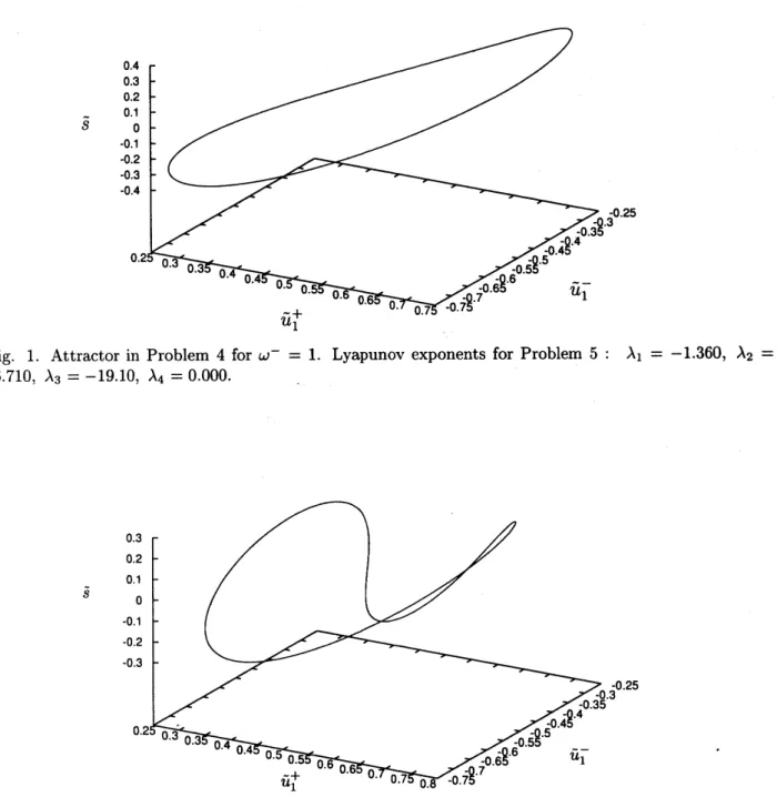
Figs. 1 -4 show attractors in the solution
space
(the
three-dimensional
space)
and
Lyapunov exponents.
Attractors
are
computed
from Problem 4. Lyapunov
exponents
are
computed
from both Problem
5and
its
linearized problem[17].
$\tilde{s}$
Fig.
1. Attractor
in
Problem
4for
$\omega^{-}=1$. Lyapunov
exponents for
Problem 5:
$\lambda_{1}=$-1.360,
$\lambda_{2}=$-6.710,
$\lambda_{3}=$-19.10,
$\lambda_{4}=0.000$.
$\tilde{s}$
Fig. 2. Attractor
in
Problem 4for
$\omega^{-}=2$. Lyapunov
exponents
for Problem 5:
$\lambda_{1}=-1.275$
,
$\lambda_{2}=$-7.487,
$\lambda_{3}=$-14.71,
$\lambda_{4}=0.000$.
$s$
Fig.
3. Attractor
in
Problem
4for
$\omega^{-}=3$.
Lyapunov
exponents
for Problem
5:
$\lambda_{1}=$-1.284,
$\lambda_{2}=$-7.264,
$\lambda_{3}=$-15.10,
$\lambda_{4}=0.000$.
$\tilde{s}$