Graphical
Methods for
$\mathrm{D}\mathrm{e}\mathrm{t}\mathrm{e}\mathrm{r}\mathrm{m}\mathrm{i}\mathrm{n}\mathrm{i}\mathrm{n}\mathrm{g}/\mathrm{E}\mathrm{s}\mathrm{t}\mathrm{i}\mathrm{m}\mathrm{a}\mathrm{t}\mathrm{i}\mathrm{n}\mathrm{g}$Optimal
Repair-Limit
Replacement
Policies
Tadashi DOHI, Kentaro
TAKEITA
and ShunjiOSAKI
Department
of Industrial and Systems
Engineering,Hiroshima
University
4-1 Kagamiyama 1
Chome,Higashi-Hiroshima 739-8527,
Japan.Abstract: In this paper, we consider two kinds of repair-limit replacement models anddevelop
the corresponding graphical methods to estimate the optimal repair-time limits which minimize the expected costs per unit time in the steady-state. Then, both the total time ontest statistics and the Lorenz statistics play important roles. Some analytical resultsarederived to describe the relationship between two models. Numerical examples are devoted to illustrate the asymptotic optimality of non-parametric estimators for the optimal repair-limit policies.
Keywords: repair-limit replacement policies, graphical methods, total time on test statistics, Lorenz statistics, partial ordering, non-parametric estimation, stochastic optimization models. 1. INTRODUCTION
Ingeneral, system maintenance models may be classified into two categories; preventive
main-tenanceandcorrective maintenance. Thepreventive maintenance is executed in advancetoavoid
a catastrophic failure state. On the other hand, the corrective maintenance is made to place
recovery actions efficiently after failures occur. The repair-limit replacement problems deter-mine how to design the recovery mechanism of a system using two maintenance alternatives;
repair and replacement, in terms of cost minimization. First this problem was considered by Hestings [1] for army vehicles and proposed three methods of optimizing therepair-limit policies
by simulation, hill-climbing and dynamic programming. Nakagawa and Osaki $[2, 3]$, Okumoto
and Osaki [4], Nguyen and Murthy $[5, 6]$ and Kaio and Osaki [7] reformulated the Hastings’
orig-inal model from the viewpoint of renewal reward processes and discussed different repair-limit replacement problems.
In themost repair-limit replacement problems [2-7], it is assumed that the distribution function of thecompletion time to repair a failed unit is arbitrary but known. This assumption seems to
be rather strong in many practical situations. To this end, practitioners have to determine the
repair-time limit under incomplete information on the repair-time distribution in most cases. Applying a graphical idea by Bergman [8] and Bergman and Klefsj\"o [9-11], the authors
[12-15] analyzed several repair-limit replacement problems and proposed the corresponding non-parametric $1\mathrm{n}\mathrm{e}\mathrm{t}\mathrm{h}_{0}\mathrm{d}_{\mathrm{S}}$ to estimate the optimal repair-time limits from the complete sample of
repair-time data.
Then $\mathrm{t}\mathrm{b}\mathrm{e}$totaltime on test (TTT) concept (see,
$e.g$. Barlow and Campo [16] andBarlow [17])
is very useful to develop the estimation procedure. In other words, some kinds of repair-limit replacement problems
are
reduced to the well-known age replacement-type $1$)$\mathrm{r}\mathrm{o}\mathrm{b}\mathrm{l}\mathrm{e}\mathrm{m}[8- 11]$ andcan
be solved by the similar graphical technique based on the TTT concept. However, such aspecific method does not always available for all maintenance problems. For instance, if the cost
criterion such as the expected cost per unit time in the steady-state can not be represented by
two variables; the repair-time distribution function and the associated scaled TTT transform,
the method mentioned above will lose its usefulness. Hence, alternative devices instead of the TTT statistics should be applied to the graphical and non-parametric estimation method for different types of maintenance problems.
In this paper, we propose estimation methods based on the Lorenz
curve
as well as the TTT statistics for two repair-limit replacement problems. The Lorenz curve was introduced first by Lorenz [18] in Economics to describe income distributions. Since the Lorenzcurve
isessentially equivalent to the Pareto curve used in the quality control, it will be one of the most importantstatistics in every social science. The more general and tractable definition of the Lorenz curve
was
made by Gastwirth [19]. Goldie [20] proved the strong consistency of the empirical Lorenzcurve
and discovered several convergence properties of it. Chandra and Singpurwalla [21] andKlefsj\"o [22] investigated the relationship between the TTT statistics and the Lorenz statistics and derived afewaging and partial ordering properties. Recently, Aly [23] developed the testing for the Lorenz ordering.
It should be noted that the underlying repair-limit replacement problems have to be analyzed by using different devices from their cost structure, respectively. In other words, both devices
are not used at the same time. The paper is organized as follows. In Section 2, we introduce two repair-limit replacement problems considered by Nakagawa and Osaki $[2, 3]$ and develop
the corresponding graphical methods to derive the optimal repair-time limits which minimize the expected costs per unit time in the steady-state. In Section 3, we obtain the comparative results to describe the relationship between two models. In Section 4, the statistical estimation problems are discussed. We show analytically and numerically that estimators of the optimal repair-time limits have strong consistency. Finally, the paper is concluded with some remarks. 2. REPAIR-LIMIT REPLACEMENT MODELS
2.1 Model 1
Consider a single unit system, where each spare is provided only by an order after a lead time $L(>0)$ and each failed unit is repairable. The original unit begins operating at time $0$. The mean lifetime for each unit is $1/\lambda(>0)$. $\backslash \mathbb{R}\mathrm{e}\mathrm{n}$ the unit has failed, the repair is started
immediately. If the repair is completed up to the time limit for repair $t_{0}\in[0, \infty)$, then the
unit is installed at that time. It is assumed that the unit once repaired is presumed as good as
new. However, if the repair time is greater than $t_{0},$ $i.e$. the repair is not completed after the
time $t_{0}$, the repair is retired and the failed unit is scrapped. Then, the spare unit is ordered
immediately and delivered after thelead time $L$. Thetime required forreplacement is negligible
for convenience. Therepair time foreach unit hasanarbitrary distribution$G(t)$withdensity$g(t)$
and finite mean $1/\mu(>0)$, where the function $G(\cdot)$ is assumed to have an inverse function, $i.e$. $G^{-1}(\cdot)$, and to be absolutely continuous and strictly increasing. Without any loss ofgenerality,
we assume $G(\mathrm{O})=0$ and $\lim_{tarrow\infty^{G}}(t)=1$
.
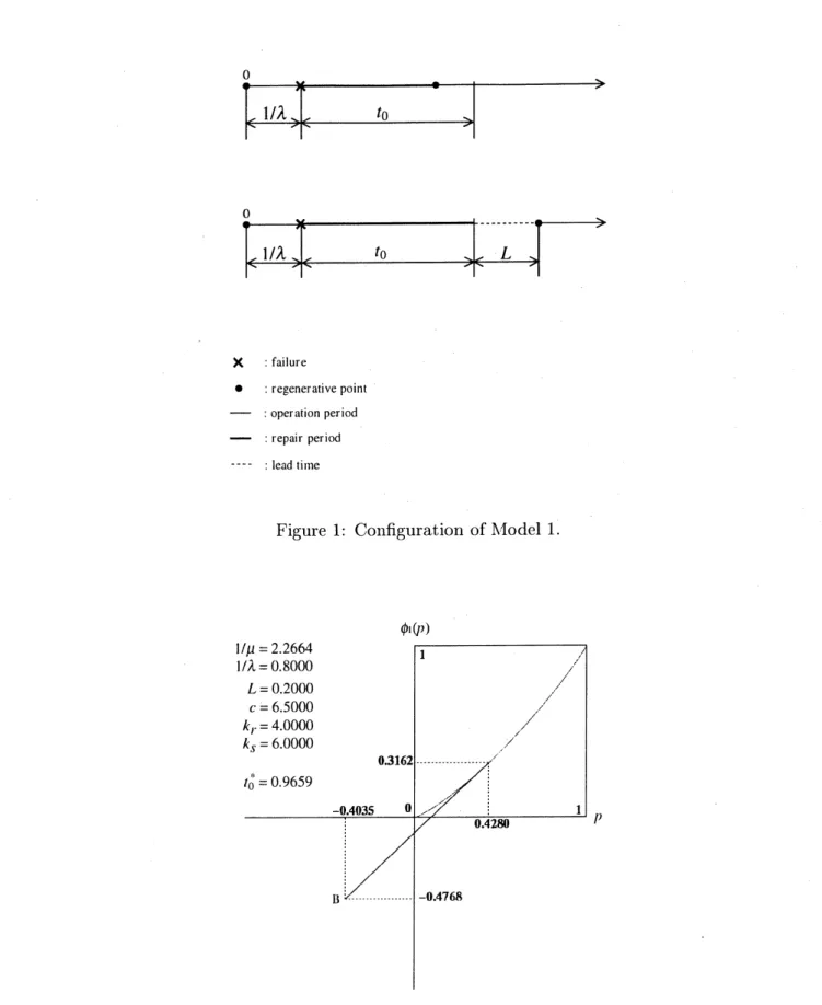
Under these model assumptions, we define the timeinterval from thestart ofthe operation to the following start as one cycle. The configuration of Model 1 is depicted in Fig. 1.
Next, we consider the cost structure. The costs considered in this paper are the following;
$k_{r}(>0)$: a cost per unit repair time $k_{s}(>0)$: acost per shortage period
$c(>0)$: an ordering cost for each spare unit. We make the $\mathrm{a}\mathrm{s}\mathrm{s}\mathrm{U}\mathrm{l}\mathrm{n}\mathrm{p}\mathrm{t}\mathrm{i}_{\mathrm{o}\mathrm{n};}$
(A-1) $k_{r}L<c$.
This assumption implies that the unit ordering cost is greater than the repair cost during the interval $[0, L],\dot{i}.e$. until the delivery ofa new unit. For an infinite planning horizon, it will be
appropriate to adopt an expected cost per unit time in the steady-state. Since the mean time of
one-
cycle is$=$ $1/ \lambda+\int_{0}^{t_{0}}\overline{G}(t)dt+L\overline{G}(t_{0})$ (1)
and the total expected cost for one cycle is
$V_{1}(t_{0})=(k_{r}+k_{s}) \int_{0}^{t}0_{\overline{G}(}t)dt+(k_{s}L+c)\overline{G}(t_{0})$, (2)
where $\overline{G}(t)=1-G(t)$, then the cost per unit time in the steady-state is, from the well-known
renewal reward argument [24, p. 52],
$C_{1}(t_{0})$ $\equiv$ $\lim_{tarrow\infty}\frac{[\mathrm{t}\mathrm{h}\mathrm{e}\mathrm{t}\mathrm{o}\mathrm{t}\mathrm{a}\mathrm{l}\mathrm{c}\mathrm{o}\mathrm{s}\mathrm{t}\mathrm{o}\mathrm{n}(0,t]]}{t}$
$=$ $V_{1}(t_{0})/T_{1}(t_{0})$ (3)
and the problem is to determine the optimal repair-time limit $t_{0^{*}}$ such as
$C_{1}(t^{*} \mathrm{o})=\min_{<0\leq t0\infty}C1(t_{0)}.$ (4)
It is straightforwardto seek $t_{0}^{*}$ bydifferentiating $C_{1}(t_{0})$ withrespect to$t_{0}$, but wehere employ
the following graphical method. Define the scaled total time on test (TTT) transform of the repair-time distribution$p\equiv G(t)$ by
$\phi_{1}(p)\equiv\mu\int_{0}^{G^{-1}(p})(\overline{G}t)dt$, $(0\leq p\leq 1)$, (5)
where
$G^{-1}(p)= \inf\{t\geq 0:G(t)\geq p\}$. (6)
The curve $p_{1}=(p, \phi_{1}(p))\in[0,1]\cross[0,1]$ is called the scaled $TTT$
transform
orsimply the scaled $TTT$ curve. We shall propose a graphical method to solve the problem in $\mathrm{E}\mathrm{q}.(4)$ on the scaledTTT curve.
The following result is due to Koshimae, Dohi, Kaio and Osaki [13].
THEOREM 2.1: Suppose the assumption (A-1) for Model 1. The minimization problem in
$\mathrm{E}\mathrm{q}.(4)$ is equivalent to obtain $p^{*}(0\leq p^{*}\leq 1)$ satisfying
$\min_{0\leq p\leq 1}:\Lambda\ell_{1}(p, \phi 1(p))\equiv\frac{\phi_{1}(p)+\xi}{p+\eta}$, (7)
where
$\xi\equiv\frac{(k_{S}L+c,)\mu}{(c-k_{\Gamma}L)\lambda}>0$ (8) and
$\eta\equiv-(1+\frac{(k_{\Gamma}+k_{S})}{(k_{r}L-c)\lambda})$
.
(9)From THEOREM 2.1, theoptimal policy is$p^{*}=G(t^{*})0$ which minimizes the tangent slope from
$(-\eta_{1}, -\xi_{1})$ to the
curve
$\ell_{1}$.
DEFINITION 2.2: (1) The repair-time distribution $G(t)$ is IHR (DHR) if and only if the
hazard rate $r(t)=g(t)/\overline{G}(t)$ is increasing (decreasing).
(2) $G(t)$ is IHR (DHR) if and only if$\phi_{1}(p)$ is concave (convex) in$p\in[0,1]$
.
The relationship (2) between the aging and the scaled TTT transform was proved by Barlow and Campo [16]. In the plane $(x, y)=(-\infty, +\infty)\cross(-\infty, +\infty)$, define the following three
p.oints
$\mathrm{B}\equiv(x_{B,y_{B})}=(-\eta, -\xi)$, (10)
$\mathrm{Z}\equiv(xz, yz)=(\frac{(k_{S}L+c)r(\mathrm{o})}{(k_{r}L-c)\lambda},$$-\xi)$ (11)
and
$\mathrm{I}\equiv(x_{I}, y_{I})=(-\eta,$$1+ \frac{(k_{r}+k_{f^{)\mu}}}{(k_{r}L-c)\lambda r(\infty)})$. (12)
THEOREM 2.3: (1) Suppose that the scaled TTT
curve
$\ell_{1}$ is strictlyconvex
under theassumption (A-1).
(i) If$x_{B}>x_{Z}$ and $y_{B}>y_{I}$, then there exists a uniqueoptimal solution $p^{*}=G(t^{*})0(0<t_{0}^{*}<$
$\infty)$ minimizing theexpected cost per unit time in thesteady-state givenby Eq. (3), where $p^{*}$ is given by the $x$-coordinate in the point of contact for the curve $\ell_{1}$ from the point $\mathrm{B}$,
where
$\max(\mathrm{O}, -\eta)<p^{*}<1$. (13)
(ii) If$x_{B}\leq x_{Z}$, then the optimal repair-limit policy is $p^{*}=G(0)=0$.
(iii) If$y_{B}\leq y_{l}$, then the optimal repair-limit policy is$p^{*}=G(\infty)=1$.
(2) Suppose that the scaled TTT curve $p_{1}$ is concave under the assumption (A-1). Then, the
optimal solution is$p^{*}=0$ or$p^{*}=1$
.
PROOF: Differentiating $\Lambda l_{1}(p, \phi_{1}(p))$ with respect to $p$ and setting it equal to zero implies
$q_{1}(p)\equiv\phi_{1}(p)’(p+\eta)-(\phi_{1()\xi)}p+=0,$ (14)
where
$\phi_{1}(p)’=\frac{\mu}{r(G^{-1}(p))}$ (15)
and tlle symbol ’ denotes the differentiation. Further, we have
$q1(p)’=\phi 1(p)\prime\prime(p+\eta)$. (16)
XVhen the scaled TTT curve $\ell_{1}$ is strictly colllrex. then $q_{1}(p)’>0$ and the $\mathrm{f}\mathrm{i}_{111}\mathrm{c}\mathrm{t}\mathrm{i}_{0\mathfrak{U}}$ A$I_{1}$(p.$\phi_{1}(p)$)
is strictly convex in $p$.
In the plane $(x, y)\in(-\infty, +\infty)\cross(-\infty, +\infty)$, we define the poirlt $\mathrm{B}=(x_{B}, y_{B})$. Since the
tangent line for the point $(p^{*}, \phi_{1}(p^{*}))$ on the curve $\ell_{1}$ is
$y= \frac{\mu}{r(G^{-1}(p^{*}))}(p-p^{*})+\phi 1(p^{*})$, (17)
the condition that thepoint$\mathrm{B}$ isover the above tangent line is$q_{1}(p^{*})=0$. Define theintersection
$x$-coordinate of$\mathrm{B}$ is strictly greater than the$x$-coordinate of$\mathrm{Z},$ $q_{1}(0)<0$, otherwise, $q_{1}(0)\geq 0$
under the assumption (A-1). Similarly, define the intersection $\mathrm{I}=(x_{I)}y_{I})$ ofthe tangent line
for the point $\mathrm{U}=(1,1)$ on the $p_{1}$ and
$x=-\eta$
.
If the $y$-coordinate of$\mathrm{B}$ is strictly greater than
the $y$-coordinate of $\mathrm{Z},$ $q_{1}(1)>0$, otherwise, $q_{1}(1)\leq 0$ under (A-1). From these, we obtain the
results (1).
Secondly, consider thecase where $G(t)$ isIHR. In this case, $\phi_{1}(p)$ becomes a
concave
functionof$p$. If the $x$-coordinate of $\mathrm{B}$ is strictly negative and if the slope of the straight line BO is
strictly smaller than that of the line $\mathrm{B}\mathrm{U}$, we have
$(k_{S}L+c)/\lambda-\{k_{r}L-c+(k_{r}+ks)\}/\mu<0$, (18)
which is equivalent to the condition of $M_{1}(0, \phi_{1}(0))<\mathbb{J}I_{1}(1,$ $\phi_{1())}1$. Conversely, if $x_{B}<0$
and if the slope of the straight line BO is not small than that of the line $\mathrm{B}\mathrm{U},$ $M_{1}(0, \phi_{1}(0))\geq$
$M_{1}(1, \phi_{1}(1))$ is satisfied. On the other hand, the condition $x_{B}\geq 0$ implies $M_{1}(0, \phi_{1}(0))\geq$
$\lambda l_{1}(1, \phi_{1}(1))$. Thus the proof is completed.
EXAMPLE 2.4: Nguyen and Murthy [6] and Dohi, Matsushima, Kaio and Osaki [14]
con-sidered the repair-limit replacement models with imperfect repair. Suppose that the repair is
imperfect. The mean lifetime when the repair is completed is $1/\lambda_{1}(>0)$. Also, a new unit
de-livered after ordering fails for aninfinite time horizon and then the mean lifetime is $1/\lambda_{2}(>0)$
.
Defining the time interval from the start of repair to the following start of repair as one cycle,
the mean time ofone cycle is
$T_{1}(t_{0})=1/ \lambda_{1}+\int_{0}^{t0_{\overline{G}}}(t)dt+(L+1/\lambda_{2}-1/\lambda 1)\overline{G}(t_{0})$. (19)
Replacing the assumption (A-1) to $k_{r}L+(k_{r}+k_{s})(1/\lambda_{2}-1/\lambda_{1})<c$, we have $\min_{0\leq p\leq 1}\sim$.
$M_{i}(p, \phi 1(p))\equiv(\phi_{1}(p)+\xi_{i})/(p+\eta_{i})$, where
$\xi_{i}\equiv\frac{(k_{S}L+cJ)\mu}{\{c-k_{\mathrm{r}}L-(k_{r}+k_{S})(1/\lambda_{2}-1/\lambda_{1})\}\lambda_{1}}>0$ (20)
and
$\eta_{i}\equiv-(1+\frac{(k_{r}+k_{s})}{\{k_{\gamma}L-C+(kr+k_{S})(1/\lambda 2-1/\lambda 1)\}\lambda})$. (21)
Therefore, the repair-limit replacement model with imperfect repair is reduced to the similar
problem with a different point $\mathrm{B}_{i}=(-\eta_{i}, -\xi_{i})$.
EXAMPLE 2.5: Suppose that the repair-time distribution is the Weibull distribution with
the shape parameter $\alpha=0.8$ and the scale parameter $\beta=2.0$
.
The other model paranletersare
$1/\lambda=$ 0.8000, $L=$ 0.2000, $c=$ 6.5000, $k_{r}=$ 4.0000 and $k_{s}=$ 6.0000. The determinationof the optimal repair-time limit for Model 1 is presented ill Fig. 2. In this case, we have $\mathrm{B}=$ $(-0.4035, - 0.4768)$ and the optimal point with $\mathrm{m}\mathrm{i}\mathrm{n}\mathrm{i}\ln\iota \mathrm{l}\mathrm{n}\mathrm{l}$ slope from $\mathrm{B}$ is $(p^{*}.\phi 1(p^{*}))=$
(0.4280, 0.3162). Tllus. the optimal repair-time limit is $t_{0}^{*}=G^{-\mathrm{l}}(0.4280)=0.9659$.
2.2 Model 2
Let $11\mathrm{S}$ consider the similar, but somewhat different model from Model 1. The original unit
begins operating at time $0$. When the unit has failed, the decision maker has to select repairor replacement. Suppose that the decision maker has asubjective probability distribution function
on the repair-completion time $G(t)$ with finite mean $1/\mu(>0)$. If he or she estimates that the
repair is completed up to the time limit $t_{0}\in[L, \infty)$, then the repair is immediately started at
the failure time. However, ifheor she estimates that the repair time is greater than $t_{0}$, then the
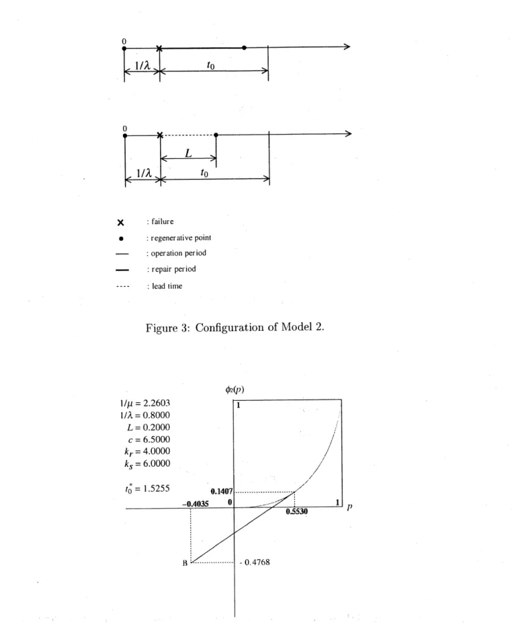
failed unit is scrapped at the failure time, the spare unit is ordered immediately and delivered after the lead time $L$. The configuration of Model 2 is illustrated in Fig. 3.
Ifwe evaluate the expected cost per unit time in the steady-state objectively, it will be $C_{2(t_{0)}}\equiv V2(t_{0})/T_{2}(t_{0})$, (22) where $V_{2}(t_{0})=(k_{S}+k_{r}) \int_{0}^{t_{0}}tdG(t)+(k_{s}L+c)\overline{G}(t\mathrm{o})$ (23) and $T_{2}(t_{0})=1/ \lambda+\int_{0}^{t_{0}}tdG(t)+L\overline{G}(t_{0})$
.
(24)Hence the problem is to determine the optimal repair-time limit $t_{0^{*}}$ such as
$C_{2}(t^{*} \mathrm{o})=0\leq t_{0}<\min_{\infty}C_{1}(t_{0})$. (25) In addition to the assumption (A-1), weneed
(A-2) $(k_{r}+k_{s})>C_{2}(t_{0})$ for $t_{0}\in[0, \infty)$
.
The assumption (A-2) will be required in order to avoid an unrealistic case. To this end, ifthe
reverse inequality holds, the repair and shortage have to always occur at the same time in the
steady-state with probability one.
To develop the similar graphical technique to Model 1, we define the Lorenz transform of the
repair-time distribution $G(t)$ by
$\phi_{2}(p)\equiv\mu\int_{0}^{G^{-1}()}p)xdG(x, (0\leq p\leq 1)$. (26)
The definition above of the Lorenz transform is essentially equivalent to
$\phi_{2}(p)=\mu\int_{0}^{p}G^{-1}(t)dt$, $(0\leq p\leq 1)$ (27)
(see [19-23]). Then thecurve $p_{2}=(p, \phi_{2}(p))\in[0,1]\cross[0,1]$ is called the Lorenz curve. From the
simple algebraic manipulation, we have
THEOREM 2.6: Suppose that the assumptions (A-1) and (A-2) hold for Model 2. The minimization problem in $\mathrm{E}\mathrm{q}.(25)$ is equivalent to
$\min_{0\leq p\leq 1}$ :
$\mathbb{J}I_{2}(p, \phi 2(p))\equiv\frac{\phi_{2}(p)+\xi}{p+\eta}$. (28)
Consequently, the optimal policy is determinedby$p^{*}=G(t^{*})0$ which lninimizesthe tangent slope
from $\mathrm{B}=(-\eta, -\xi)\in(-\infty, 0)\cross(-\infty, 0)$ to the curve $\ell_{2}$
.
PROOF: The expected cost per unit time in the steady-state in $\mathrm{E}\mathrm{q}.(22)$ becolnes $C_{2}(t_{0)}=$ $(k_{s}+k_{r})-K(t_{0})$, where
$K(t_{0}) \equiv\frac{(k_{S}+k_{r})\mu/\lambda+\mu(krL-c)\overline{c}(t_{0})}{\mu/\lambda+\mu L\overline{G}(t\mathrm{o})+\int_{0}\iota_{0}tdG(t)}$
.
(29)Since $K(t_{0})>0$ for $t_{0}\in[0, \infty)$ from (A-2), it is found that $(k_{s}+k_{r})/\lambda>c-k_{r}L$ from (A-1)
THEOREM 2.7: (1) Suppose that the assumptions (A-1) and (A-2) hold. Thenthereexists
a
unique optimal solution$p^{*}=G(t_{0}*)(0<t_{0}^{*}<\infty)$ minimizing the expected cost per unit time in
the steady-stategiven by Eq. (28), where$p^{*}$ is givenby the$x$-coordinate in the point ofcontact
for the
curve
$\ell_{2}$ from the point B.PROOF: Differentiating $M_{2}(p, \phi_{2}(p))$ with respect to $p$ and setting it equal to zero implies
$q_{2}(p)\equiv\phi_{2}(p)’(p+\eta)-(\phi_{2()\xi)}p+,$ (30)
where $\phi_{2}(p)’=\mu G-1(p)$. Further, we have
$q_{2}(p)^{;}=\phi 2(p)’’(p+\eta)>0$ (31)
and the function $\Lambda I_{2}(p, \phi_{2}(p))$ is strictly convex in $p$, since $\phi_{2}(p)\prime\prime=\mu/g(G^{-1}(p))>0$. From
$q_{2}(0)=-\xi<0$ and $q_{2}(1)arrow\infty$, the result is proved.
EXAMPLE 2.8: Suppose that the repair-time distribution is the Weibull distribution with
the shape parameter $\alpha=0.8$ and the scale parameter $\beta=2.0$
.
The other model parametersare
$1/\lambda=$ 0.8000, $L=$ 0.2000, $c=$ 6.5000, $k_{r}=$ 4.0000 and $k_{s}=$ 6.0000. The determinationof the optimal repair-time limit for Model 2 is presented in Fig. 4. In this case, we have $\mathrm{B}=$ $(-0.4035, - 0.4768)$ and the optimal point with minimum slope from $\mathrm{B}$ is $(p^{*}, \phi_{2}(p^{*}))=$
(0.5530, 0.1407). Thus, the optimal repair-time limit is $t_{0}^{*}=G^{-1}(0.5530)=1.5255$.
3. COMPARATIVE RESULTS
We compare two repair-limit replacement models. From Eqs. (3) and (22), it can be seen
that $T_{1}(t_{0})=T_{2}(t_{0})+t_{0}\overline{G}(t0)$ and$V_{1}(t_{0})=V_{2}(t_{0})+(k_{r}+k_{s})t0\overline{G}(t_{0})$ for afixed $t_{0}$. When $t_{0}=0$
and $t_{0}arrow\infty$, it is obvious that $C_{1}$$(to)=C_{2}$(to). Thus, we pay our attention to the case of$t_{0}\in$
$(0, \infty)$
.
Now, define $C_{1}(t_{1}^{*})= \min_{0<t_{0}<1}\infty C(t_{0}),$ $C_{2}(t_{2}^{*})= \min 0<t_{0}<\infty C2(t_{0)}$, A$f_{1}(p_{1}^{*}, \phi_{1}(p_{1}^{*}))=$$\min_{0<p1}<$
All
$(p, \phi_{1}(p))$ and $\Lambda l_{2}(p^{*}2’\phi 2(p_{2}^{*}))=\mathrm{m}\mathrm{i}\mathrm{n}0<p<1\mathbb{J}I2(p, \phi 2(\overline{p}))$.THEOREM 3.1: (i) Under the assumption (A-2), $C_{1}(t_{0})>C_{2}(t_{0})$ holds for a fixed$t_{0}\in[0, \infty)$.
(ii) Under the assumptions (A-1) and (A-2), if$\phi_{j}(p)(j=1,2)$ is monotonically increasing and
strictly
convex
in$p\in(0,1)$, then$p_{1}^{*}<p_{2}^{*}$ and $t_{1}^{*}<t_{2}^{*}$.
PROOF: (i) $C_{1}(t_{0})>C_{2}(t_{0})$ if and only if $(k_{r}+k_{S})t_{0}\overline{c}(t0)T2$(to) $>t_{0}\overline{G}(t\mathrm{o})V_{2}$(to). Since
$t_{0}\overline{G}(t_{0})>0$forafixed$t_{0}\in(0, \infty)$ and (A-2), the result is derived. (ii) Chandra and Singpurwalla
[21] proved the following relation;
$\phi_{1}(p)=\phi_{2}(p)+\mu(1-p)c^{-1}(p)$. (32)
Hence, we $\mathrm{h}\mathrm{a}\backslash r\mathrm{c}\phi_{1}(p)>\phi_{2}(p)$ for $p\in(0,1)$. Since $\phi_{j}(p)(j=1,2)$ is monotonically increasing
and strictly convex in $p\in(0.1)$, it is straightforward to see $p_{1}^{*}<p_{2}^{*}$ and $t_{1}^{*}<t_{2}^{*}$. The proof is
completed.
Next, we develop the $\mathrm{c}\mathrm{o}\ln_{\mathrm{I}^{)}}\mathrm{a}\mathrm{r}\mathrm{a}\mathrm{t}\mathrm{i}\backslash r\mathrm{c}$results on respective repair-linlit replacement models.
Sup-pose that there are two repairmen with different repair abilities. We classify two repairmen into Repairman 1 and Repairman 2, respectively. Their repair times $X_{1}$ and $X_{2}$ are non-negative
$\mathrm{r}\mathrm{a}\mathrm{n}\mathrm{d}_{0}$
. $\mathrm{m}$ variables with distribution functions $G_{j}(t)(j=1,2)$ and the same
$\mathrm{f}\mathrm{i}\mathrm{n}\mathrm{i}\mathrm{t}_{r}\mathrm{e}$ mean $1/\mu$,
respectively. $1^{1}\dagger^{\mathrm{r}_{\mathrm{e}}}$ require the following definition on the stochastic ordering [25].
DEFINITION
3.2: (1) $X_{1}$ is usuallystochastic-orderedwith respect to$\lambda_{2}’$ (denotedas $X_{1}\leq_{\mathrm{s}\mathrm{t}}$$X_{2})$ if$\overline{c_{1}}(t)\leq\overline{G_{2}}(t)$.
(2) $X_{1}$ is star-shapedstochastic-orderedwith respect to$X_{2}$ (denotedas$X_{1}\leq_{*}X_{2}$) if$G_{2}^{-1}(G_{1}(t))/t$ is increasing in $t\in(\mathrm{O}, G_{1}^{-1}(1))$.
THEOREM 3.3: In Model 1, define the optimal repair-time limits for two repairmen with
the same mean repair time $1/\mu$ as $t_{11}^{*}=G_{1}^{-1}(p_{11}^{*})$ and $t_{12}^{*}=G_{2}^{-1}(p_{1}^{*}2)$, respectively, where $p_{11}^{*}$
and$p_{12}^{*}$ are the solutions for Eq. (7) with $G_{j}(t)(j=1,2)$
.
If$\phi_{1}(p)$ is monotonically increasingand strictly convex in$p\in[0,1]$ and if the repair time for Repairman 1 is smaller than that for
Repairman 2 in the usual stochastic ordering, then$t_{11}^{*}\leq t_{12}^{*}$.
PROOF: From the well-known result by Barlow [17], we find that $\phi_{1}(G_{1}(t))\geq\phi_{1}(c_{2}(t))$
if.
andonly if$X_{1}\leq_{*}X_{2}$. Immediately, we have $p_{11}^{*}\leq p_{12}^{*},$ $G_{1}(t_{1}^{*})1\leq G_{2}(t_{12}^{*})$ and $G_{2}^{-1}(G_{1}(t_{11}^{*}))\leq t_{12}^{*}$,
since$\phi_{1}(p)$ is monotonically increasing and strictlyconvexin$p\in[0,1]$. Sincethe usual stochastic
ordering $\leq_{\mathrm{s}\mathrm{t}}$ includes the star-shaped ordering $\leq*’ c_{2}^{-1}(c_{1}(t^{*})11)\leq t_{12}^{*}$ and $G_{1}(t)\geq G_{2}(t)$ yield
$G_{1}(t_{1}^{*})1\leq G_{2}(t_{1}^{*})2$ and $t_{11}^{*}\leq t_{12}^{*}$.
THEOREM 3.4: In Model 2, definethe optimal repair-time limits for two repairmenwith the
same mean repair time $1/\mu$ as $t_{21}^{*}=G_{1}^{-1}(p_{21}^{*})$ and $t_{22}^{*}=G_{2}^{-1}(p_{22}^{*})$, respectively, where $p_{21}^{*}$ and
$p_{22}^{*}$ are the solutions for Eq. (28) with $G_{j}(t)(j=1,2)$
.
If the repair time for Repairman 1 issmaller than that for Repairman 2 in the usual stochastic ordering, then $t_{21}^{*}\leq t_{22}^{*}$
.
PROOF: Chandra and Singpurwalla [21] proved $\phi_{2}(G_{1}(t))\geq\phi_{2}(G_{2(}t))$ if$X_{1}\leq*X_{2}$. Therest
part ofthe proofis similar to THEOREM 3.3.
4. NON-PARAMETRIC ESTIMATION METHODS
Based on the graphical ideas in Section 2, we propose statistical methods to estimate the
optimal repair-limit policies for two models. Suppose that the optimal repair-time limit has to be estimated from an ordered complete sample $0=x_{0}\leq x_{1}\leq x_{2}\leq\cdots\leq x_{n}$ ofrepair times
from an $\mathrm{a}\mathrm{b}_{\mathrm{S}\mathrm{O}}1\acute{\mathrm{u}}\mathrm{t}\mathrm{e}\mathrm{l}\mathrm{y}$continuous repair-time distribution $G$, which is unknown. The estimator of
$G(t)=p$ is the empirical distribution given by $G_{n}(_{X)}=\{$
$i/n$ for $x_{i}\leq x<x_{i+1}$, $(i=0,1,2, \cdots, n-1)$
(33)
1 for $x_{n}\leq x$
.
Then the scaled TTT statistics based on this sample are
$\phi_{1i}\equiv S_{i}/S_{n}$, (34)
where
$S_{i} \equiv\sum_{i=1}^{i}(n-j+1)(x_{jj-1}-x)$, $(\dot{i}=1,2, \cdots, n;S_{0}=0)$. (35)
By plotting the point $(\dot{i}/n, \phi_{1i}),$ $(\dot{i}=0,1,2, \cdots, n)$, and connecting them by line segments, we
obtain the so-called scaled $TTT$ plot, $\ell_{1n}\in[0,1]\cross[0,1]$. On the other hand, the empirical
Lorenz curve is
$\phi_{2i}\equiv\sum_{1i=}^{]}x_{i}/\sum_{i=1}^{n}X_{i}[np$, (36) where $[0]$ is the greatest $\mathrm{i}_{11\mathrm{t}(}$)
$\mathrm{g}\mathrm{e}\mathrm{r}$ ill $a.$ Silllilarl}r, plotting tlle point $(i/r\}, \phi_{\mathit{2}i}),$ $(i=0.1,2, \cdots , n)$, andconnecting them by linesegments, we obtain the empiricalLorenz curve $\ell_{2n}\in[0,1]\cross[0,1]$.
As empirical counterparts of THEOREM 2.1 and THEOREM 2.6, we propose non-parametric estimators of the repair-time limits for respective models.
THEOREM 4.1: The optimal repair-time limit for Model $j(=1,2)$ can be estimated by $t_{jn}\wedge=x_{i^{*}}$, where
The proof is omitted for brevity. We consider the following two examples for better understand-ing of the result above.
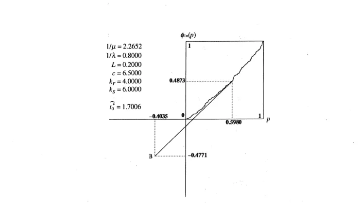
EXAMPLE 4.2: The repair-time datawere made by the random number following the Weibull
distribution withshapeparameter$\alpha=0.2$and scale parameter$\beta=2.0$. The other model
param-eters
are
$1/\lambda=0.8000,$ $L=0.2000,$ $c=6.5000,$ $k_{r}=4.0000$ and $k_{s}=6.0000$.
The scaled TTTplotbasedonthe 200sampledata for Model 1 is shown in Fig. 5. Since$\mathrm{B}=$ $(-0.4035, - 0.4771)$, the optimal point with minimum slope from $\mathrm{B}$ becomes $(\dot{i}^{*}/n, \phi_{1i}*)=$ $($119/200,$\phi_{1,119})$ –
(0.5980, 0.4873). Thus, the estimator of the optimal repair-time limit $\hat{t}_{1,20}0=x_{119}=1.7006$.
EXAMPLE 4.3: Under the same model parameters with EXAMPLE 4.2 except for $\alpha=$
$0.8$, the empirical Lorenz curve based on the 200 sample data for Model 2 is shown in Fig.
6. Since $\mathrm{B}=$ $(-0.4035, - 0.4771)$, the optimal point with minimum slope from $\mathrm{B}$ becomes
$(\dot{i}^{*}/n, \phi_{2i^{*}})=$ $($110/200,$\phi_{2,110})=$ (0.5829, 0.1742). Thus, the estimator of the optimal
repair-time limit $\hat{t}_{2,200=X_{11}}0=1.6492$
.
Ofour interest is the investigation of asymptotic properties of the estimators $\hat{t}_{jn},$ $(j=1,2)$ in
THEOREM 4.1. The following theorem guarantees the asymptotic optimality of the $\mathrm{e}\mathrm{s}\mathrm{t}\mathrm{i}\mathrm{n}\mathrm{l}\mathrm{a}\mathrm{t}_{0}\mathrm{r}\mathrm{S}$
above.
THEOREM 4.4: (i) The expected cost $C_{j}(t_{jn})\wedge,$ $(j=1,2)$ of using the repair-time limit $\hat{t}_{jn}$
may be estimated by
$\hat{C}_{j}(t_{j}^{*})7\mathrm{t}--\frac{(k_{r}+kS)\phi_{j(p)}jn*/\mu n+(k_{S}L+c)(1-p_{j}^{*}n)}{1/\lambda+\phi_{j}(pjn)*/\mu n+L(1-p_{jn})}$, (38) where $1/\mu_{n}$ is empirical mean of the repair time. Then the estimator is strongly consistent.
(iii) If aunique optimal repair-time limit exists then $\hat{t}_{jn}(j=1,2)$ is strongly consistent.
PROOF: See for $j=1$ (Model 1) Bergman [8]. For$j=2$ (Model 2), it is straightforward from
convergence theorems for empirical Lorenz curve proved by Goldie [20].
We examine numerically the strong consistency of estimators proposed for two repair-limit
replacement models. Since the realoptimal repair-time limit canbe calculated underthe known
repair-time distribution, we investigatethe convergence property of estimators to the realvalue.
EXAMPLE 4.5: For Model 1, suppose that the repair-time distribution is the Weibull
dis-tribution with the shape parameter $\alpha=0.2$ and $\mathrm{t}_{)}\mathrm{h}\mathrm{e}$ scale parameter $\beta=2.0$. The other $\mathrm{T}\mathrm{h}\mathrm{e}\mathrm{n}\mathrm{t}\mathrm{h}\mathrm{m}\mathrm{o}\mathrm{d}\mathrm{e}1\mathrm{p}\mathrm{a}\mathrm{r}\mathrm{a}\mathrm{m}\mathrm{e}\mathrm{t}\mathrm{e}\mathrm{r}_{1\mathrm{p}\mathrm{e}\mathrm{C}}\mathrm{s}\mathrm{a}\mathrm{r}\mathrm{e}\mathrm{l}/\lambda=0.8000,L=0.2000,c\mathrm{e}\mathrm{o}\mathrm{p}\mathrm{t}\mathrm{i}\mathrm{m}\mathrm{a}\mathrm{r}\mathrm{C}\mathrm{a}\mathrm{i}\Gamma- \mathrm{t}\mathrm{i}\mathrm{m}\mathrm{e}\mathrm{l}\mathrm{i}\mathrm{m}\mathrm{i}\mathrm{t}\mathrm{a}\mathrm{n}\mathrm{d}\mathrm{t}\mathrm{h}\mathrm{e}\mathrm{m}\mathrm{i}\mathrm{n}\mathrm{i}\mathrm{n}\mathrm{l}\mathrm{u}\mathrm{m}=6.5\mathrm{o}\mathrm{o}\mathrm{t}\exp \mathrm{e}\mathrm{d}0,k_{r,\mathrm{c}}=\mathrm{o}\mathrm{s}\mathrm{t}\mathrm{b}\mathrm{e}4.0\mathrm{o}\mathrm{o}0\mathrm{a}\mathrm{n}\mathrm{d}\mathrm{C}\mathrm{o}\mathrm{m}\mathrm{e}t_{0}*0=1ks.6=29^{\cdot}9\mathrm{a}\mathrm{n}\mathrm{o}\mathrm{o}\mathrm{o}0\mathrm{d}$
.
$C_{1}(t_{0}^{*})=0.2050,$ $\mathrm{r}\mathrm{e}\mathrm{s}\mathrm{p}\mathrm{e}\mathrm{c}\mathrm{t}\text{ノ}\mathrm{i}\mathrm{l}\prime \mathrm{e}\mathrm{l}\mathrm{y}$. On the $\mathrm{o}\mathrm{t}$,her hand, the asymptotic behaviour of estimators for
the optimal repair-time limit and their associated lninim\iota lln $\mathrm{e}\mathrm{x}\mathrm{p}\mathrm{e}\mathrm{c}\mathrm{f}_{7}\mathrm{e}\mathrm{d}$ costs are depicted in Figs. 7 and 8. $\mathrm{F}\mathrm{r}\mathrm{o}\ln$ these figures, we observe $\mathrm{t}_{J}\mathrm{h}\mathrm{a}\mathrm{t}$ the $\mathrm{e}\mathrm{s}\mathrm{t}\mathrm{i}\mathrm{l}\mathrm{n}\mathrm{a}\mathrm{t}_{\mathrm{O}}\mathrm{r}\mathrm{S}$ converge to the corresponding real
values around which the number of data is 50.
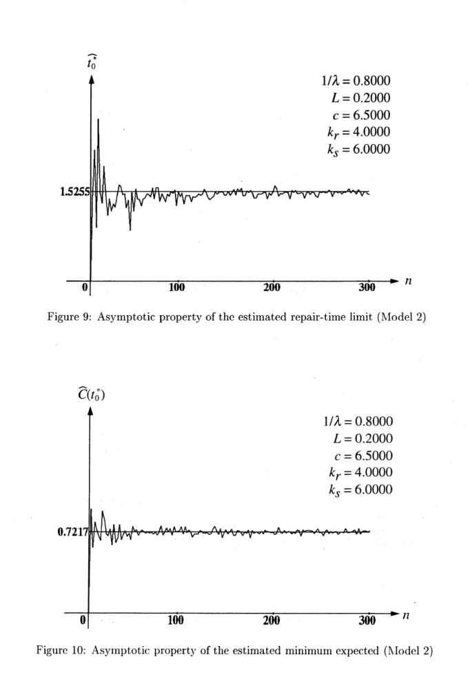
EXAMPLE 4.6: For $\mathrm{I}\backslash \mathrm{I}\mathrm{o}\mathrm{d}\mathrm{e}\mathrm{l}2$, suppose that tlle repair-tinlc distribution is tlle XVeibull $\mathrm{d}\mathrm{i}\mathrm{s}\mathrm{t}\mathrm{l}\cdot \mathrm{i}-$
bution with the shape $1$)
$\mathrm{a}\mathrm{r}\mathrm{a}\mathrm{m}\mathrm{G}\mathrm{t}\mathrm{e}\mathrm{r}\alpha=0.8$alld the scale parameter $\beta=2.0$. The other model
parameters
are
similar toEXAMPLE 3.5. Then the optimal repair-time limit and the mininuurn expected cost become $t_{0}^{*}=$ 1.5255 and $C_{2}(t_{0}*)=$ 0.7217, respectively. On$\mathrm{t}_{\mathit{1}}\mathrm{h}\mathrm{e}$ other hand, the
asymptotic behaviour of estimators for the optimal repair-time limit and their associated min-imum expected costs are depicted in Figs. 9 and 10. From these figures, we observe that the
estimators converge to the corresponding real values around which the number of data is 80.
In this paper, we have proposed graphical methods toestimate the optimal repair-time limits for two kinds of repair-limit replacement models, based on the total time on test statistics and the Lorenz statistics. It has been shown that both estimators provided are non-parametric and have strong consistency. These statistical properties will be usefulfor practitioners to determine the $\mathrm{m}\dot{\mathrm{a}}\mathrm{i}\mathrm{n}\mathrm{t}\mathrm{e}\mathrm{n}\mathrm{a}\mathrm{n}\mathrm{C}\mathrm{e}$plan if they can obtain a sufficiently large number of repair-time data. If we have to determine the optimal repair-limit policy from small sample, then any statistical
technique such as Jack-Knife method should be applied to make the number of given sample
increase or existing parametric methods should be used to specify the repair-time distribution with some theoretical distribution functions.
References
[1] Hastings, N. A. J., $‘(\mathrm{T}\mathrm{h}\mathrm{e}$repair $\acute{\lim}$it replacement method”, Operational Research Quarterly,
vol. 20, pp. 337-349 (1969).
[2] Nakagawa, T. and Osaki, S., $‘(\mathrm{T}\mathrm{h}\mathrm{e}$ optimum repair limit replacement policies”, Operational
Research Quarterly, vol. 25, pp. 311-317 (1974).
[3] Nakagawa, T. and Osaki, S., “Optimum ordering policies with lead time for an operating
unit”, R.A.I.R.0. Recherche $Op\dot{e}rat\dot{i}onnelle/o_{pera}t\dot{i}onS$ Research, vol. 12, pp. 383-393
(1978).
[4] Okumoto, K. and Osaki, S., “Repair limit replacement policies with lead time”,
Zeitschrift
fiir
Operations Research, vol. 20, pp. 133-142 (1976).[5] Nguyen, D. G. and Murthy, D. N. P., ((A note on the repair limit replacement policy”,
Journal
of
Operational Research Society, vol. 31, pp. 1103-1104 (1980).[6] Nguyen, D. G. and Murthy, D. N. P., (‘Optimal repair limit replacement policies with im-perfect repair”, Journal
of
Operational Research Society, vol. 32, pp. 409-416 (1981).[7] Kaio, N. andOsaki, S., ((Optimumrepair limit policies withatimeconstraint”, International
Journal
of
Systems Science, vol. 13, pp. 1345-1350 (1982).[8] Bergman, B., “Onage replacement and the total time on test concept”, Scandinavian
Jour-nal
of
Statistics, vol. 6, pp. 161-168 (1979).[9] Bergman, B. and Klefsj\"o, B., “A graphical method applicable toagereplacement problems”, IEEE Transactions on Reliability, vol. R-31, pp. 478-481 (1982).
[10] Bergman, B. and Klefsj\"o, B., “TTT-transforms and age replacements with discounted
costs”, Naval Research Logistics Quarterly, vol. 30, pp. 631-639 (1983).
[11] Bergman, B. and $\mathrm{K}\mathrm{l}\mathrm{e}\mathrm{f}\mathrm{s}\mathrm{j}_{\ddot{\mathrm{O}}}$, B., “The total time on test concept and its use in reliability
theory”, Operations Research, vol. 32, pp. 596-607 (1984).
[12] Dohi, T., Kaio, N. and Osaki, S., “Solution procedure for a repair limit problem using
TTT-transform”. IMA Journal
of
Mathematics, Appli,ed Business and Industry, vol. 6,pp. 101-111 (1995).
[13] Koshimae, H., Dohi, T., Kaio, N. and Osaki, S., $‘\prime \mathrm{G}\mathrm{r}\mathrm{a}\mathrm{p}\mathrm{h}\mathrm{i}\mathrm{C}\mathrm{a}1/\mathrm{s}\mathrm{t}\mathrm{a}\mathrm{t}\mathrm{i}_{\mathrm{S}\mathrm{t}}\mathrm{i}\mathrm{c}\mathrm{a}1$ approach to repair
limit replacement problem”, $Jou\gamma\cdot nal$
of
the Operations Research Societyof
Japan, vol. 39,pp. 230-246 (1996).
[14] Dohi, T., Matsushima, N., Kaio, N. and Osaki, S., “Non-parametric repair limit
replace-ment policies with imperfect repair”, European Journal
of
Operational Research, vol. 96,[15] Dohi, T., Koshimae, H., Kaio, N. and Osaki, S., “Geometrical interpretations of repair cost limit replacement policies”, International Journal
of
Reliability, Quality and Safety Engineering, vol. 4, pp. 309-333 (1997).[16] Barlow, R. E. and Campo, R., “Total time on test processes and applications to failure
data analysis”, Reliability and Fault Tree Analysis (R. E. Barlow, J. Fussell and N. D. Singpurwalla, eds.), pp. 451-481, SIAM, Philadelphia (1975).
[17] Barlow, R. E., “Geometry of the total time on test transform”, Naval Research Logistics,
vol. 26, pp. 393-402 (1979).
[18] Lorenz, M. O., $‘\zeta \mathrm{M}\mathrm{e}\mathrm{t}\mathrm{h}_{0}\mathrm{d}\mathrm{s}$ ofmeasuring the concentration ofwealth”) Journal
of
AmericanStatistical Association, vol. 9, pp. 209-219 (1893).
[19] Gastwirth, J. L., “A general definition of the Lorenz curve”, Econometrica, vol. 39, pp.
1037-1039 (1971).
[20] Goldie, C. M., (
$‘ \mathrm{C}_{\mathrm{o}\mathrm{n}\mathrm{V}\mathrm{e}\mathrm{r}}\mathrm{g}\mathrm{e}\mathrm{n}\mathrm{c}\mathrm{e}$ theorems for empirical Lorenz curves and their inverses”,
Advances in Applied Probability, vol. 9, pp. 765-791 (1977).
[21] Chandra, M. and Singpurwalla, N. D., “Relationship between some notions which are
common to reliability and economics”, Mathematics
of
Operations Research, vol. 6, pp.113-121 (1981).
[22] Klefsj\"o, B., “Reliability interpretations ofsomeconcepts from economics”, NavalResearch Logistics Quarterly, vol. 31, pp. 301-308 (1984).
[23] Aly, E. A. A., (‘On testing for Lorenz ordering”, Metrika, vol. 38, pp. 117-124 (1991).
[24] Ross, S. M., Applied Probability Models with Optimization Applications, Holden-Day, San
X failure
$\bullet$ regenerative point
– operation period
– repair period
– leadtime
Figure 1: Configuration of Model 1.
Figure 2: Determination of the optimal repair-time limit based on the scaled TTT transform
X failule
$\bullet$ $1^{\cdot}\mathrm{e}\mathrm{g}\mathrm{e}\mathrm{n}\mathrm{e}\mathrm{r}\mathrm{a}\iota \mathrm{i}\mathrm{V}\mathrm{e}$point
operation period
– repair$\mathrm{p}\mathrm{e}\mathrm{l}$iod
lead time
Figure 3: Configuration of Model 2.
$d_{\mathrm{I}},/\mathrm{n}\mathrm{Y}$
Figure 4: Determination of the optimal repair-time limit based on the Lorenz transform (Model
Figure 5: Estimation of the optimal repair-time limit based on the scaled TTT plot (Model 1).
Figure6: Estimation of the optimal repair-time limit basedontheempirical Lorenz curve (AIodel 2).
Figure 7: Asymptotic property of the estimated repair-time limit (Model 1)
’(t ハ
$\overline{*}$
$t_{\cap}$
Figure 9: Asymptotic property ofthe estimated repair-time limit (Model 2)
$(^{\neg}\vee(f_{\cap^{*}}\wedge)$