The B\’enard
Problem
of Rarefied Gas DynamicsYoshio Sone, Kazuo Aoki, Hiroshi Sugimoto, and Hideto Motohashi
(gRB$*$, $\ovalbox{\tt\small REJECT}*$
-g,
bit #, $*\hslash\ovalbox{\tt\small REJECT}$A)Division
ofAeronautics
and Astronautics,Graduate School of Engineering, Kyoto University,
Kyoto 606-01, Japan
Abstract
Thetwo-dimensionalB\’enardproblem of ararefiedgasin arectangular domain
is studied numerically by a
finite-difference
analysis of theBoltzmann-Krook-Welander equation. The diffuse reflection is assumed on the upper cooled wall
and on the lower heated wall and the specular reflection on the sideboundaries.
The range of the parameters where a convection exists, steady flow patterns, a
bifurcation of flow pattern, and a process of
convergence
to an array of uniform size rolls are presented.I. Introduction
The B\’enard problem conceming the instability of a layer offluid heated from below has
long been of interest to many scientists and engineers, and a lot of works have been done
on the basis of the continuum
theoryl-5.
The study of the problem of a rarefiedgas
isjust at a starting point, and only a few
works6,
which their authors call preliminary, havebeen done by the direct simulation Monte Carlo
method78.
In a series of papers we willstudy the problem more systematically and try to obtain more comprehensive result of the
problem. In the present paper we consider the two-dimensional B\’enard problem of a rarefied
gas in a rectangular
domain
and investigate the condition (the range of the parametersflow. Numerical analysis by afinite-differencemethod on the basis of the
Boltzmann-Krook-Welander $equation^{8-10}$ is chosen to pursue the problem.
II.
Problem
and basicequation
Inthispaper we considertwo dimensional flows of a rarefied
gas
in arectangulardomain
($0<X_{1}<L,$ $0<X_{2}<D;X_{i}$ is the Cartesian coordinate system), where the
gas
is subjectto a uniform gravitational force in the negative $X_{2}$ direction, the lower boundary at $X_{2}=0$
is heated at a uniform temperature $T_{h}$, and the upper at $X_{2}=D$ is cooled at a
uniform
temperature $T_{c}$
.
We analyze the behavior ofthegas
under the following assumptions:i$)$ The behavior of the gas is described by the Boltzmann-Krook-Welander equation.
ii) The molecules make the diffuse reflection on the upper and lower boundaries.
iii) The molecules make the specular reflection on the side boundaries at $X_{1}=0$ and $L$
.
The Boltzmann-Krook-Welanderequation is given by
$\frac{\partial f}{\partial t}+\xi_{1}\frac{\partial f}{\partial X_{1}}+\xi_{2}\frac{\partial f}{\partial X_{2}}-g\frac{\partial f}{\partial\xi_{2}}=A_{c}\rho(f_{e}-f)$ , (1)
$f_{e}= \frac{\rho}{(2\pi RT)^{3/2}}\exp(-\frac{(\xi_{i}-v_{i})^{2}}{2RT})$, (2)
$\rho=\int fd\xi_{1}d\xi_{2}d\xi_{3}$, (3a)
$v_{i}= \rho^{-1}\int\xi_{i}fd\xi_{1}d\xi_{2}d\xi_{3}$, (3b)
$3RT= \rho^{-1}\int(\xi_{i}-v_{i})^{2}fd\xi_{1}d\xi_{2}d\xi_{3}$
.
(3c)Here, thenotations are as follows: $t$ isthe time; $\xi_{i}$ is themolecular velocity; $f$is the velocity
distribution function; $\rho$ is the density of the
gas;
$v_{i}$ is the flow velocity $(v_{3}=0)$ of thegas; $T$ is the temperature of the gas; $g$ is the acceleration ofgravity; $A_{c}$ is a constant $(A_{c}\rho$
is the collision frequency of a molecule, which is common to all the molecules in the
case
ofthe Boltzmann-Krook-Welander model); $R$ is the specific
gas
constant. The integrals inThe boundary conditions on the upper and lower boundaries are, at $X_{2}=0$,
$f=\rho h(2\pi RT_{h})^{-3/2}\exp(-\xi_{i}^{2}/2RT_{h})$, $(\xi_{2}>0)$, (4a)
$\rho h=-(2\pi/RT_{h})^{1/2}\int_{\xi_{2}<0}\xi_{2}fd\xi_{1}d\xi_{2}d\xi_{3}$, (4b)
and, at $X_{2}=D$,
$f=\rho_{c}(2\pi RT_{c})^{-3/2}\exp(-\xi_{i}^{2}/2RT_{c})$, $(\xi_{2}<0)$
,
(5a)$\rho_{c}=(2\pi/RT_{c})^{1/2}\int_{\xi_{2}>0}\xi_{2}fd\xi_{1}d\xi_{2}d\xi_{3}$
.
(5b)The boundary conditions on the side boundaries are, at $X_{1}=0$
,
$f(X_{1}, X_{2}, t, \xi_{1}, \xi_{2}, \xi_{3})=f(X_{1},X_{2}, t, -\xi_{1}, \xi_{2}, \xi_{3})$, $(\xi_{1}>0)$, (6)
and, at $X_{1}=L$,
$f(X_{1},X_{2}, t, \xi_{1}, \xi_{2}, \xi_{3})=f(X_{1},X_{2}, t, -\xi_{1}, \xi_{2}, \xi_{3})$, $(\xi_{1}<0)$. (7)
Theinitial condition is, at $t=0$
,
$f=f_{0}$, (8)
where $f_{0}$ is properly chosen.
By use ofproperly chosennondimensionalvariables, Eqs. (1)$-(3c)$ and the boundary
con-ditions $(4a)-(7)$ are reduced to a system characterized by the four parameters: the Knudsen
number $Kn[=(8RT_{0}/\pi)^{1/2}(A_{c}\rho_{0})^{-1}D^{-1}=\ell_{0}/D]$, the Froude number $Fr(=2RT_{h}/Dg)$, the
temperature ratio $T_{c}/T_{h}$, and the aspect ratio $L/D$, where $\rho_{0}$ is the average density of the
gas
over the domain,$l_{0}$ is themeanbeepath of the state$f_{e}$ [in Eq.(2)].with
$\rho=\rho_{0},$ $T=T_{h}$,and $v_{i}=0$
.
Equations (1)$-(3c)$ withtheboundary condition $(4a)-(7)$ hasa time-independent solution
without flow $(v_{i}\equiv 0)$ for any set of the parameters. Let it be $f_{s}(X_{2}, \xi_{i})$ and let the
corresponding density and temperature be $\rho_{s}(X_{2})$ and $T_{s}(X_{2})$
.
When the gravity is strong(when $Fr$ is large), $\rho_{s}$ increases with $X_{2}$
.
In the intermediate gravity (intermediate $Fr$),$\rho_{s}$ first decreases with $X_{2}$, reaches its minimum, and then increases. Our interest is the
possibility of another type of solutions with nonzero flow velocity, such as a steady solution
of aconvection roll, in ararefied gas. Thus, we numerically analyze the initial and
boundary-value problem (1)$-(7)$ for many sets of parameters and investigate the range of parameters
where solutions with flow exist, and their flow pattern. Further, we present an example of
flow bifurcation, i.e., approach to different types of steady solutions from slightly
different
initial conditions.
The independent variable $\xi_{3}$ can be eliminated from the system (1)$-(7)$, if we are
satis-fied with the information of the marginal distribution functions $\int_{-\infty}^{\infty}fd\xi_{3}$ and $\int_{-\infty}^{\infty}\xi_{3}^{2}fd\xi_{3}$
.
The system for these quantities is obtained by integrating Eq. (1), (4a), (5a), (6), and (7)
multiplied by $l$ or $\xi_{3}^{2}$ with respect to $\xi_{3}$ over $(-\infty<\xi_{3}<\infty)$. In the present work, we carry
out a standard finite-difference numerical analysis ofthis system.
III. Existence
range
of nonstationary solutions and their flow patternsIn order to find the range of the parameters $(Fr,$ $T_{c}/T_{h}$, etc.$)$ where a flow occurs in
the rectangular domain, we investigate the initial and boundary-value problem (1)$-(7)$ for
many sets of the parameters and pursue thelong-time behaviorofthe solution. Asthe initial
distribution function $f_{0}$ in Eq. (8), we take the Maxwellian distribution:
$f_{0}=\rho(2\pi RT)^{-3/2}\exp(-\xi_{i}^{2}/2RT)$,
(9)
$\rho=\rho_{s}(X_{2})$, $T=T_{s}(X_{2})[1+(1/2)\cos(\pi X_{1}/L)\sin(\pi X_{2}/D)]$,
where$\rho_{s}(X_{2})$ and $T_{s}(X_{2})$ are the density and temperature ofthe stationary solution for the
corresponding values of the parameters. (It is noted that the Maxwellian distribution with
$\rho_{s}$ and $T_{s}$ is not the solution of Eq. (1) owing to its gravitational term.)
Pursuing thelong-time behavior of the solution of theinitialandboundary-value problem
(1)$-(7)$, we find that the solution approaches the corresponding stationary solution $f_{s}$ or
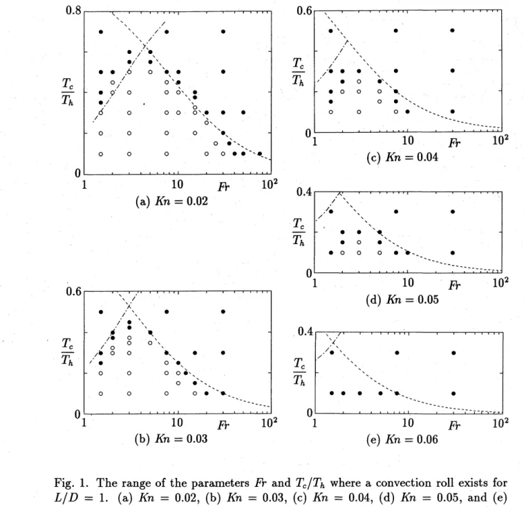
parameter range of the two class of solutions is shown in Figs. 1-3, where the stationary solution is marked by $\bullet$ and the steady solution of a convection roll by $0$ in the $(I\dagger_{2}T_{c}/T_{h})$
plane. Fig. 1 is the result at $Kn=0.02,0.03,0.04,0.05$, and
0.06
in the square domain$L/D=1$
,
Fig. 2 is the result at $Kn=0.02$ in thedomain
$L/D=3/4$, and Fig.3
is
the resultat $Kn=0.02$ in the domain$L/D=1/2$
.
A steadyconvectionroll of flowexists ina triangularregion in the $(Ik, T_{c}/T_{h})$ plane, and it rapidly shrinks as the Knudsen number increases.
According to the linear stability
analysis5
based on the continuumtheory, $Ra=$ 1700, where$Ra=(16/\pi)(1-T_{c}/T_{h})/(T_{c}/T_{h})FrKn^{2}$ (Rayleigh number), isthe critical value above which
the stationary solution is unstable. In Fig. 1 the curve $Ra=1700$ is shownby a dashedline.
As mentioned in
Sec.
II, the density $\rho_{s}(X_{2})$ of a stationarysolution
decreases monotonicallyas $X_{2}$ increases for small $F\succ$, but has its minimum in the gas for intermediate Fr. The
approximate boundary ofthese regions is shown by a chain linein Fig. 1.
The computationis carriedout onlyfora specialinitial condition. Thus,in thetriangular region with $0$ sign, a single roll of steady flow certainly exists, but another type offlowmay
occur. In fact we will show suchexamples, besidesthe reversal $f(L-X_{1}, X_{2}, -\xi_{1}, \xi_{2}, \xi_{3})$of
a
solution.
$f(X_{1}, X_{2}, \xi_{1}, \xi_{2}, \xi_{3})$, inSec.
IV. In theregion
with $\bullet$ sign, the existence of a flowcannot be excluded, but various tests, although they are not systematic but are randomly carried out, show that occurrence of a perpetual flow is improbable.
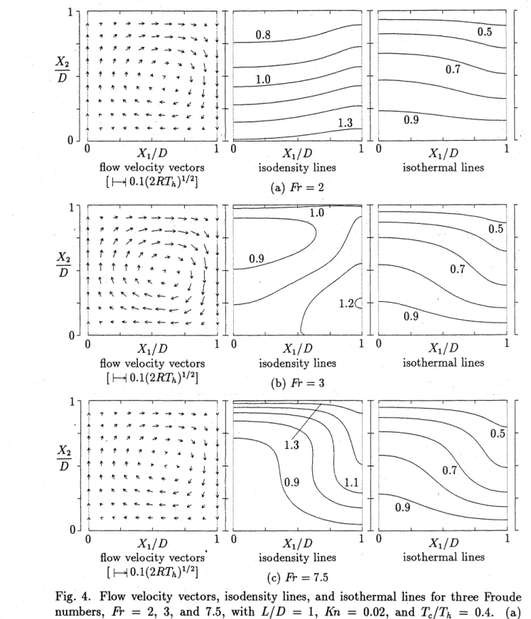
Example of flow fields (flow velocity vectors, isodensity lines, and isothermal lines) in
the case of $L/D=1$ are shown in Figs. 4 and 5. In Fig. 4 the results at $Kn=0.02$
and $T_{c}/T_{h}=0.4$ are shown for three typical Froude numbers $Fr=2,3$ , and 7.5, which
correspond to three different types of $\rho_{s}(X_{2})$ mentioned in
Sec.
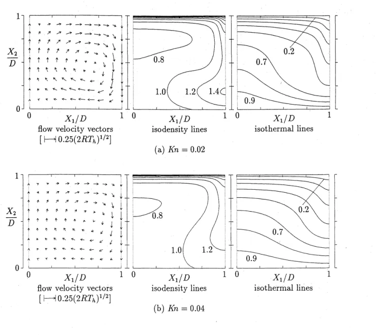
II. In Fig.5
the resultsfor two different Knudsen numbers, $Kn=0.02$ and 0.04 with the other parameters being
common $(T_{c}/T_{h}=0.1, Fr=3)$ are shown. The lateral position of the center of the roll
is nearly at $X_{1}=2L/3$ for all the cases in Figs. 4 and 5, but its vertical position differs
IV. Array of rolls and
bifurcation
of flowA steady solution of Eq. (1) extended across a specularly reflecting plane boundary
by joining its mirror image or reversal (i.e. extended symmetrically with respect to the
boundary)
can
be shown to be a solution ofEq. (1) in a wider domain. Thus, by arranginga series of steady solutions of a kind laterally in such a way that adjacent solutions are the mirror images of each other, we can construct a steady solution in a wider domain. The
array $f_{a}^{N}$ of $N$ steady solutions ofa single roll $f_{a}$ in the domain with $L/D=a$ so arranged
forms a solution consisting of$N$ rolls in the domain $L/D=Na$
.
For example both $f_{3/4}^{4}$ and$f_{1}^{3}$ are solutions in the domain $L/D=3$
.
Our next interest is bifurcation to these different types of flow. Taking, as the initial
condition $f_{0}$ in the initial and boundary value problem (1)$-(7)$ in the domain $L/D=k\ell/m$,
$f_{0}=\alpha f_{k/m}^{\ell}+(1-\alpha)f_{\ell/m}^{k}$ , (10)
where $\alpha$ is a constant $(0\leq\alpha\leq 1)$ and $k,$ $\ell$, and $m$ are positive integers, we pursue the
time-development of the solution and investigate the type of thelimiting solution as $tarrow\infty$
for different $\alpha$
.
Here wegivesomeresults inthe domain $L/D=3$for the initial condition (10) with$\ell=4$,
$k=3$
,
and $m=4$for $Fr=3$ and $T_{c}/T_{h}=0.1$.
When $Kn=0.02$, the solution approaches $f_{1}^{3}$for $\alpha=0.6$ but $f_{3/4}^{4}$ for $\alpha=0.7$; when $Kn=0.03$
,
it approaches $f_{1}^{3}$ for $\alpha=0.8$ but$f_{3/4}^{4}$ for
$\alpha=0.9$; when $Kn=0.04$, even for $\alpha=0.99$, it approaches $f_{1}^{3}$
.
Several tests indicate thatif $farrow f_{3/4}^{4}$ for $\alpha_{1}$, then $farrow f_{3/4}^{4}$ for $\alpha\geq\alpha_{1}$ and that if $farrow f_{1}^{3}$ for $\alpha_{2}$, then $farrow f_{1}^{3}$ for
References
1. B\’enard, H. (1900): Les tourbillons cellulaires dans une nappe liquide. Revue G\’en. Sci.
Pur. Appl., 11, 1261-1271,
1309-1328.
2. Rayleigh, L. (1916): On convectioncurrents inahorizontallayer offluid whenthehigher temperature is on the under side. Phil. Mag., 32,
529-546.
3. Busse, F. H. and Clever, R. M. (1979): Instabilities of convection rolls in a fluid of
moderate Prandtl number. J. Fluid Mech., 91, 319-335.
4. Mizushima, J. and Fujimura, K. (1992): Higher harmonic resonance of two-dimensional
distributions in Rayleigh-B\’enard convection. J. Fluid Mech., 234,
651-667.
5.
Koschmieder, E. L. (1993): B\’enard Cells and Taylor Vortices. CambridgeUniv.
Press,Cambridge.
6. Cercignani, C. and Stefanov, S. (1992): B\’enard’s instability in kinetic theory. Transp.
Theory Stat. Phys., 21, 371-381; Stefanov, S. and Cercignani, C. (1992): Monte Carlo
simulation ofB\’enard’s instabilityin a rarefiedgas. Eur. J. Mech.f B/Fluids, 11, 543-554.
7.
Bird,G.
A. (1976): MolecularGas
Dynamics. Clarendon Press, Oxford.8. Sone, Y. and Aoki, K. (1994): Molecular Gas Dynamics (Appendix II). Asakura, Tokyo.
9. Bhatnagar, P. L., Gross, E. P. and Krook, M. (1954): A model for collision processes in
gases,
I. Phys. Rev., 94, 511-525.0.8
.
$\backslash \backslash \backslash \backslash \backslash \backslash$ $\backslash \rangle_{\backslash }/\cdot/\cdot$$/\cdot\cdot\backslash$
:/
$\cdot$ $\backslash \backslash$
.
$.$ $6$ $0\backslash \backslash \cdot$$\frac{T_{c}}{T_{h}}$
$0_{/}’$ $0_{\backslash }^{\backslash }$
.
$9^{\cdot}$ $0$ $0$ \‘o$\backslash$$\backslash \cdot$ $\backslash \cdot$ /
$/d$ $oo$
$\backslash o_{\backslash }o_{\backslash }\circ$
$\cdot$ $\cdot$ $0$ \‘O$\backslash$ $0$ $0$ $0$ $0$ $\backslash$
.
$0$ $\backslash \backslash _{s}$$0$ $0$ $0$ $0$ $0\circ\cdot\backslash \sim\backslash \backslash -$
$0$
1
10
$10^{2}$$Fr$
($a$) $Kn=0.02$
0.6
$\backslash c_{\wedge}./\backslash \cdot$ /$\cdot\backslash$ $\backslash$
$\cdot$ /
$\cdot$ $:\backslash \backslash \backslash$
$\underline{T_{c}}$ $/\dot{\cdot}O/\cdot O/$ ’ $s$ $oo$ $\circ\langle\backslash$ $0$ $\backslash$ $T_{h}$ / $\cdot$
$oo\backslash 0_{\backslash }^{\backslash }\grave{.}$ $0$ $0$
$0$ $\backslash _{s}\backslash \backslash$ $0$ $0$ $0$ $0\cdot\sim$
.
-$\sim$ -$——-$ $0_{1}$ 10 $Fr$ $10^{2}$ ($b$) $Kn=0.03$0.6
$\backslash \backslash \backslash \iota\backslash \backslash$
.
$f_{c}$$/’/\cdot/\cdot/\backslash \backslash \backslash$
$\frac{T_{c}}{T_{h}}$
$’$
.
$0_{\backslash }^{\backslash }\backslash \backslash \backslash \grave{\cdot}\backslash \cdot$
.
$0$ $0$ $0\backslash c$ $0$ $\backslash \sim\backslash _{s}$ $\backslash _{s}$ $0$ $0$ $0$.
$\backslash --\sim$ $-\sim\wedge-$ $——–$ $0_{1}$10
$Fr$ $10^{2}$ ($c$) $Kn=0.04$ 0.4 $/^{\iota}\backslash \backslash$/’/. $\backslash \backslash \backslash \backslash \backslash$ $\cdot$ $\frac{T_{c}}{T_{h}}$ $c$
.
$\backslash \backslash$ $0$ $s_{c}$ $s_{\vee}$ $\circ 0$ $0$ $0$ $\sim\backslash .--$ $-$ $—-$ $—-$ $0_{1}$10
$——- 10^{2}$ $Fr$ ($d$) $Kn=0.05$ 0.4$/\cdot/\backslash \backslash l_{\backslash }’\backslash \backslash \backslash$
.
$\frac{T_{c}}{T_{h}}$$\backslash \backslash \backslash \backslash \backslash \backslash s_{Y}\sim$ $s\backslash$
.
$-$ $\sim_{s}$ $-\backslash$ $—$ $0_{1}$ 10 $———– Fr^{10^{2}}$ ($e$) $Kn=0.06$Fig. 1. The range of the parameters $Fr$ and $T_{c}/T_{h}$ where a convection roll exists for
$L/D=1$
.
(a) $Kn=0.02,$ $(b)Kn=0.03,$ $(c)Kn=0.04,$ $(d)Kn=0.05$ , and (e)$Kn=0.06.0$ : Convection occurs; $\bullet$ : No flow
occurs.
See the second paragraph inSec. III for $—-$ and –. [The $(X_{1}, X_{2})$ space is divided into $24\cross 24$ nonuniform
rectangular lattices finer near the upper and right boundaries. The $(\xi_{1},\xi_{2})$ space,
limited to $|\xi_{1}|$ and $|\xi_{2}|\leq 4(2RT_{h})^{1/2}$, is divided into 40x40 nonuniform rectangular
Fig. 4. Flow velocity vectors, isodensity lines, and isothermal lines for three Froude
numbers,
$Fr=2,3$,
and 7.5, with $L/D=1,$ $Kn=0.02$, and $T_{c}/T_{h}=0.4$.
(a)$F\succ=2,$ $(b)Fr=3$, and (c) $Fr=7.5$
.
The arrows indicate the velocity at theirstarting points. The contours $\rho/\rho 0=0.1n$ and $T/T_{h}=0.1n$ are shown. [The $(X_{1}, X_{2})$
space is divided into $48\cross 48$ [in (a) and $(b)$] or $72\cross 72$ [in $(c)$] nonuniform rectangular
lattices finer near the upper and right boundaries. The $(\xi_{1},\xi_{2})$ space, limited to $|\xi_{1}|$ and $|\xi_{2}|\leq 4(2RT_{h})^{1/2}$
,
is divided into $40\cross 80$ [in $(a)$], $40\cross 60$ [in $(b)$], or $40\cross 40$ [in $(c)$]Fig. 5. Flow velocity vectors, isodensity lines, and isothermal lines for two Knudsen
numbers, $Kn=0.02$ and 0.04, with $L/D=1,$ $Fr=3$
,
and $T_{c}/T_{h}=0.1$. $(a)Kn=0.02$and (b) $Kn=0.04$
.
The arrows indicate the velocity at their starting points. Thecontours $\rho/\rho_{0}=0.2n$ and $T/T_{h}=0.1n$ are shown. $[$The $(X_{1},$$X_{2})$ space is divided into
$48\cross 56$ nonuniform rectangular lattices finer near the upper and right boundaries. The
$(\xi_{1}, \xi_{2})$ space, limited to $|\xi_{1}|$ and $|\xi_{2}|\leq 4(2RT_{h})^{1/2}$, is divided into $40\cross 60$ nonuniform
$=0$ $=100$ $=440$ $(2RT_{h})^{1/2}D^{-1}t$ $=500$ $\wedge 7$ $(2RT_{h})^{1/2}D^{-1^{\frac{X_{2}}{D}}}t$
$\uparrow ffl\nearrow\nearrow Barrowarrow\searrow tk\wedge z\nearrowarrowarrowarrowarrow\sim\searrow\uparrow\uparrow\uparrow\uparrow\dagger 4_{7\Delta}\uparrow fffl\nearrow zarrow\Rightarrow\searrow*kkR\nwarrow\nwarrow\simarrow l\uparrow it\nwarrow R\kappa_{r\iota_{l)^{\downarrow}}}^{V}A\triangleright s\nwarrow\approxarrowarrowarrow<\swarrow[\swarrow<\approxarrow<arrow x\kappa\kappa\wedge.n44l_{\psi^{Apk}}^{\swarrow<<\sim\nwarrow I\nwarrow\aleph 4}\{\Downarrow s\tau flflflflf\uparrow\{\cdot 4\nwarrow\nwarrow\aleph\searrowarrowarrowarrowarrowarrow B74\wedge\iota\searrow\swarrow\Leftarrow\epsilon R\nwarrow\nwarrow t\uparrow\uparrow f7t\prime zt\uparrow\uparrow\uparrow\uparrow\uparrow\uparrow\phi\phi’$
$=2300$
$01$
$\frac{A<arrow\divarrowarrow>7A\mapsto i1arrowarrowarrowarrowarrowarrow s\psi z<-arrowarrowarrow\wedge\epsilon rA\tau\geqarrowarrowarrowarrowarrowarrow 3\psiarrow\nearrow\nearrow\nearrow\nearrow l44k\aleph R\nwarrow\nwarrow\simarrow\swarrow\sqrt{}\uparrow\phi fl\nearrow\nearrowarrow\simarrow\searrow trs\nwarrow<<<-<\swarrow z\nearrowarrow\simarrowarrow\sim\searrow\downarrow\theta L7^{\vee}\Delta u4\searrow\}^{\downarrow}\downarrow}{0123X_{1}/D}\ovalbox{\tt\small REJECT}$
$[\mapsto 0.25(2RT_{h})^{1/2}]$
(a) $\alpha=0.6$
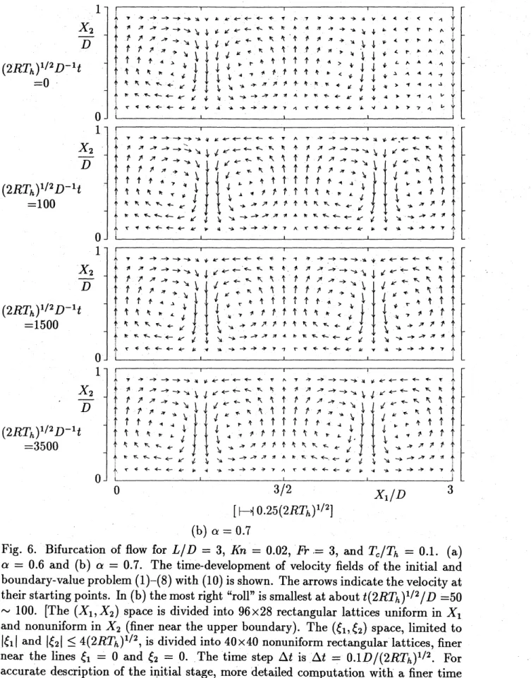
$=0$ $=100$ $=1500$ $=3500$ $[\mapsto 0.25(2RT_{h})^{1/2}]$ (b) $\alpha=0.7$
Fig. 6. Bifurcation of flow for $L/D=3,$ $Kn=0.02,$ $Fr=3$, and $T_{c}/T_{h}=0.1$
.
(a)$\alpha=0.6$ and (b) $\alpha=0.7$
.
The time-development of velocity fields of the initial andboundary-valueproblem (1)$-(8)$ with(10) is shown. The
arrows
indicate thevelocityat their starting points. In (b) themost right “roll” is smallest at about$t(2RT_{h})^{1/2}/D=50$$\sim 100$. [The $(X_{1},X_{2})$ space is divided into $96\cross 28$ rectangular lattices uniform in $X_{1}$
and nonuniform in $X_{2}$ (finer near the upper boundary). The $(\xi_{1},$$\xi_{2}\}$ space, limited to $|\xi_{1}|$ and $|\xi_{2}|\leq 4(2RT_{h})^{1/2}$, is divided into $40\cross 40$ nonuniform rectangular lattices, finer
near the lines $\xi_{1}=0$ and $\xi_{2}=0$
.
The time step $\Delta t$ is $\Delta t=0.1D/(2RT_{h})^{1/2}$.
Foraccurate description of the initial stage, more detailed computation with a finer time