Continuous, Discrete, Ultradiscrete Waves (Interfaces, Pulses and Waves in Nonlinear Dissipative Systems : RIMS Project 2000 "Reaction-diffusion systems : theory and applications")

(1)

Continuous, Discrete,

Ultradiscrete

Waves

TAKAHASHI Daisuke (

高橋大輔

)

Dept.

of Mathematical Sciences, (

数理科学科

)

Waseda Univ. (

早稲

大学

)

1 Introduction to Ultradiscretization

‘Ultradiscretization’ is a technique to discretize dependent variable of

differ-ence equations. Using this technique, we can obtain universal mathematical

structure among differentialequations, difference equations and digital equa-tions. The following is one example on the diffusion equation,

$g_{t}=gxx$. (1)

We have a difference analogue to the above equation,

$f_{j}^{n+1}= \frac{1}{2}(f_{j+}^{n}1+f_{j-1}n)$. (2)

If we use the following transformation,

$f_{j}^{n}=\exp(F_{j}^{n}/\epsilon)$, (3)

we obtain from (2),

$F_{j}^{n+1}=\mathcal{E}\log(e^{F_{j+1}^{n}}/\mathcal{E}+e^{F_{j}^{n}}-1/\epsilon)-\mathcal{E}\log 2$

.

(4)

Taking $\epsilonarrow+0$ and using an identity

(2)

we obtain

$F_{j}^{n+1}= \max(F_{j+1}^{n}, F_{j-1}^{n})$. (6)

Note that $F_{j}^{n}$ are always integer if initial $F$ are all integer. In this meaning,

we discretize a dependent variable in (2) and obtain (6).

In the above discretizing process, we only use atransformation of variable (3) and an identity (5). Therefore, this technique can be applied to other equations including nonlinear ones. We call this kind of discretizing process on dependent variable ‘ultradiscretization’.

The second example is Burgers equation. It is well known Burgers equa-tion can be linearized through Cole-Hopf transformation.

$\{$

$g_{t}=g_{xx}$ (diffusion eq.)

$\uparrow$ $v=(\log g)_{x}$ (Cole-Hopf trans.)

$v_{t}=2vv_{x}+v_{xx}$ (Burgers eq.)

(7)

We can obtain a difference analogue to the above system,

$|_{u_{j}}^{f_{j}^{n}}n+1n \frac{=1}{\triangle}\log(e_{\triangle xu^{n}J-}^{-\Delta x}J^{-1f)}e^{\Delta x})u^{n}u_{j+}\mathrm{t}\uparrow u\frac{1}{-1x\triangle x\{}j(n\mathrm{g}\mathrm{o}f_{j+}^{n}1\mathrm{g}j(\mathrm{d}\mathrm{i}\mathrm{f}\mathrm{f}\mathrm{e}_{\mathrm{i}}\mathrm{r}\mathrm{e}\mathrm{n}\mathrm{c}\mathrm{e}\mathrm{C}\mathrm{o}1\mathrm{e}\mathrm{H}\mathrm{o}\mathrm{p}\mathrm{f}\mathrm{r}\mathrm{a}\mathrm{o}\mathrm{n}$ S

$+1=u_{j}+= \frac{1}{2}(f_{j+1}n+f_{j-}^{n_{\mathrm{l}}}1)\mathrm{o}\mathrm{g}(e-1^{+}+e)(\mathrm{d}\mathrm{i}\mathrm{f}\mathrm{f}\mathrm{e}\mathrm{r}_{\Delta}\mathrm{e}\mathrm{n}xnu_{j}^{n}\mathrm{C}\mathrm{e}_{1}\mathrm{d}\mathrm{i}n\}\mathrm{f}\mathrm{f}\mathrm{u}\mathrm{S}\mathrm{i}_{\mathrm{o}\mathrm{n}\mathrm{e}\mathrm{q}.)}(\mathrm{d}\mathrm{f}\mathrm{f}\mathrm{e}\mathrm{r}\mathrm{e}\mathrm{n}\mathrm{C}\mathrm{e}\mathrm{B}^{-}\mathrm{u}\mathrm{r}\mathrm{g}\mathrm{e}\mathrm{r}\mathrm{S}\mathrm{e}\mathrm{q}.).)$

(8)

Moreover, if we use the following transformations of variables,

(3)

and take a limit $\epsilonarrow+0$, we obtain

$\{$

$F_{j}^{n+1}= \max(F_{j+1}^{n}, F_{j-1}^{n})$ (ultradiscrete diffusion eq.)

$\downarrow$

$U_{j}^{n}=F^{n}-F^{n}j+1j+1/2$ (ultradiscrete Cole-Hopftrans.)

$U_{j}^{n+1}=U_{j}^{n}+ \min(U_{j-1}^{n},1-U_{j}^{n})-\min(U_{j}n, 1-U_{j+1}^{n})$

(ultradiscrete Burgers eq.)

(10)

Ifall initial $U’ \mathrm{s}$ are integer in

$\mathrm{u}$-Burgers $\mathrm{e}\mathrm{q},$

$U’ \mathrm{s}$ at any time become integer.

(In this case, $F$ may be half integer but is also discretized.)

Moreover, assuming that initial $U’ \mathrm{s}$ are all $0$ or 1, we can easily show

$U’ \mathrm{s}$ at any time also become _$0$

or 1. Under this restriction of values, we can consider that $\mathrm{u}$-Burgers equation is a cellular automaton

$(\mathrm{C}\mathrm{A})$ with state

values $0$ and 1. This CA follows a time evolution rule,

$\frac{U_{j-1}^{n}U_{jj+}^{n}U^{n}1}{U_{j}^{n+1}}$ : $\frac{000}{0}\frac{001}{0}\frac{010}{0}\frac{011}{1}\frac{100}{1}\frac{101}{1}\frac{110}{0}\frac{111}{1}$, (11) and it is equivalent to the rule-184 elementary CA after Wolfram. Note

that there is a _{common linearization structure among Burgers, d-Burgers}

and $\mathrm{u}$-Burgers equations, we can propose their

explicit solutions through

diffusion equation, even to $\mathrm{u}$-Burgers equation. Especially, we can easily

show a pattern selection mechanismof rule-184 CA using the linearization.

We have already obtained various ultradiscretizable nonlinear equations and

interesting

results. Ultradiscretization gives a universal view on systems

from continuous to digital, _{and proposes a new approach to analyze their}

mathematical structure.

2

${\rm Max}$

-Plus

Equation

on

Pattern

Formation

In the previous section, we introduced successful examples of

ultradiscretiza-tion method. However, there is a weak point in the method. We usually use

transformation of variables like (3) in the

ultradiscretization.

Then,

(4)

ofdifferenceequations can be automatically ultradiscretized. When we meet

this difficulty, one of possible solutions is ‘back-ultradiscretization’, that is,

to make a CA or ultradiscrete equation first, follow thereverse path of

ultra-discretization, and obtain a continuous (differential or difference) equation.

There occurs another difficulty in this approach though

back-ultradiscre-tization is always easy. Because the continuous equation obtained often be-comes trivial. However, when there is no clue to digitalize a system, this

approach is always valuable to try.

In this section, we show a digital equation relevant to pattern formation

system. This equation is expressed by $\max$ and addition operators. Since

ultradiscrete equations are always expressed by $\max$ and addition, they are

called $‘ \max$-plus equation’ after _$\max$-plus algebra. Since we have not yet

obtained a successful back-ultradiscretization of the digital equation shown

below, we call it $\max$-plus equation, not ultradiscrete equation.

The equation is

$u_{ij}^{t+1}= \max(u_{i+}^{t}u-1j’ u_{ij}1j’ itt+1’ iu^{t}j-1’ u_{ij}^{t})-u_{i}-tjuijt-1$, (12)

where $i$ and _$j$ are space lattices and$t$ isinteger time. This equation is second

orderin timeand we can rewrite theabove equation to a system of equations offirst order using $v_{ij}^{t}=u_{ij}^{t-1}$,

$\{$

$u_{ij}^{t+1}= \max(u_{i\dagger 1j’ i-1}^{t}u^{t}u_{ij}^{t}j’+1’ u_{i}tj-1’ u_{ij}^{t})-u_{ij}-v_{i}^{t}tj$

$v_{ij}^{t+}=u_{i}^{t}1j$

(13) In this form, we may consider that it is an activator-inhibitor system. The

reason is as follows:(i) $u$ has a diffusion effect by _$\max$ term. (ii) $u$ decreases

by $v$. (iii) $v$ is equal to $u$ at a previous time step, that is, $v$ increases if $u$

increases. (iv) Thus $u$ is activator and $v$ is inhibitor.

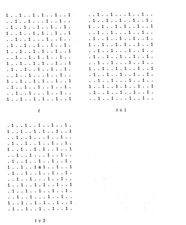
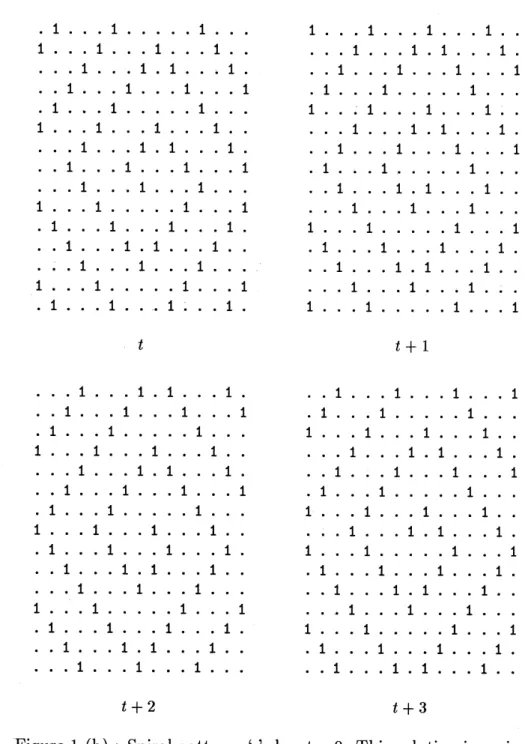
Figure 1 showstwo numerical results, Fig. 1 (a) showsatargetpattern and

(b) aspiral pattern. This pattern is often observedin some of typical pattern

formation systems, for example, reaction-diffusion systems. However, there

(5)

One is that (12) is reversible in time and the other is that if $u$ is a solution,

$Cu$ is also. Therefore, we consider that a usual reaction-diffusion system

can not be obtained by back-ultradiscretization of (12). Thus there occurs a question ‘What is a continuous system corresponding to (12)?’

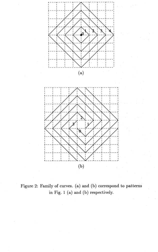
We have not yet succeeded non-trivial back-ultradiscretization of (12), we can not answer this question now. However, the above system has a remarkable feature. Let us prepare a family of curves shown in Fig. 2 (a) and (b) corresponding to Fig. 1 (a) and (b). Each curve is labeled with

an integer as shown in figures. Then, assume values of $u’ \mathrm{s}$ on curve

$n$ are the same and $f_{n}^{t}$ denotes the value on curve $n$ at time $t$. Then, from a

symmetry of (12), (12) reduces to the following one-dimensionalequation for both patterns:

$f_{n}^{t+1}= \max(f^{t}n+1’ f^{t}n’ fn-1)t-fn-f_{n}^{t}t-1$. (14)

Note that

$f_{0}^{t+1}= \max(f^{t}\mathrm{o}’ f^{t}1)-f\mathrm{o}^{t}-f\mathrm{o}^{t-1}$ (15)

is applied for $n=0$ as a boundary condition in the target pattern and $n$ becomes a periodic lattice with period 4 in the spiral pattern. Under

this difference on boundary condition, both patterns satisfy the same

one-dimensional equation exactly.

Moreover, both patterns become atravelingwave solution in (14).

There-f\"ore, we can make a reduction further. If we set a traveling wave form

$f_{n}^{t}=g_{n-t}$, we obtain

$g_{n+1}= \max(gn+1,gn’ gn-1)-_{\mathit{9}n}-gn-1$ (16)

from (14). We would emphasizethefollowings:(i) Such exact reduction is very difficult in continuous reaction-diffusion systems. (ii) The families of curves in Fig. 2 can be considered to be digital analogues to circles and spirals in a $\mathrm{c}\mathrm{o}\mathrm{n}\mathrm{t}!\mathrm{n}\mathrm{u}\mathrm{o}\mathrm{u}\mathrm{S}$ coordinate system. These points suggest (12) is related to a $\mathrm{s}\mathrm{o}1_{\mathrm{V}}\mathrm{a}\mathrm{b}\mathrm{l}\mathrm{e}$

,continuous

pattern

model.

It is an interesting future problem to

(6)

1 1

.

1

.

1

.

1

.

1 1

.

1

.

1.

.

1. 1

. .

1.

.

1.

.

1

. .

1

.

1. 1

.

1 1

.

1 1 1. 1

. . .

1

.

1

.

1 :

.

1 1

.

1

.

1 1

.

1

.

1

.

1

.

1

. .

1 1 1 1 1

.

1 1

.

1

.

1

.

1

.

1

.

1 1 1 1 1 1 1 1

.

1.

.

1. 1

. .

1

. .

1

.

1 1 1 1

.

1 1 1 1 1.

.

1 1.

.

1 1

.

1

.

1 1 1

. .

1 1 : 1

.

1 1 1

.

1 1

.

1. 1

.

1 1 1 1 1 ‘

.

1 1

.

1

.

1.

.

1

. .

1.

.

1

. .

1 1 1 1

. .

1

.

1 1

.

1

.

1 1

.

1 1 1 1 1

.

1 ,

.

1 1

. .

1

.

1

.

1. 1 1

.

1

. .

1. 1

.

1

.

1

.

1

.

1 1 1 1 1 $i$

.

1 1 1 1

.

1

.

1. 1

. .

1

. .

1 1 1

.

1 1 , 1 1

.

1

.

1.

.

1

.

$t$ $t+1$

.

1

. .

1

.

1

.

$\backslash$

.

$1$

.

1 1 1

. .

1

.

1

.

1

. .

1 1 1 1

.

1

.

1 1 1 1. 1 1.

.

1.

.

1. 1. 1.

..

1 1. 1

.

1.

.

1.

.

1

.

1.

.

1.

.

1.

.

1. 1. 1

.

1 a 1

. .

1

.

1

.

1.

.

1

.

1.

.

1.

.

1. 1

.

1

. .

1.

.

1. 1

.

1 1. 1 $*$ $\cdot$ 1

. .

1 1 1.

.

1.

.

1.

.

1 1 1.

.

1 1 1.

.

1. , _1. 1 ,

.

_1. 1 1.

.

1.

.

1. 1. 1 $t+2$

Figure 1 (a) : Target pattern. ‘.’ and $‘ \mathrm{a}$’ denote $0$ and-l respectively. This

(7)

1

.

1

.

. .

1

.

1

.

1

.

1.

.

1 1.

.

1. 1.

.

1

.

1.

. .

1.

.

1.

. .

1 1

.

. .

1

. .

.

1

. .

1.

. .

1.

.

1

. . .

1.

.

1

.

1 1

.

1

.

1

.

1.

. .

1

.

1

.

1

.

1

. .

1

.

1

.

1.

.

1.

.

1

.

1

.

1

.

1.

.

1

.

1.

.

1 1.

.

1

.

1

.

1.

.

1

.

1

.

1.

. . . .

1.

. .

1

.

1.

.

1

.

$arrow 1$

.

1. 1

.

. .

1

.

1 1 1

. . .

1

.

1.

. .

1

.

1

.

1.

. .

1

.

1

.

1.

. .

1

. . . .

.

1 1

.

. .

1

.

1

. . .

1 1

. .

1

.

1

.

. .

1

.

1 1

.

1 1

.

1

.

1 $\mathrm{r}$

. . . .

1 $*$ 1

. .

1 1

.

1.

.

1 1

.

. .

1

. .

1

. . .

1.

. . . .

1

. . .

1 1.

. .

1

. .

.

1.

.

1

. .

1

. . .

1.1

.

1

.

1

. . .

1

. .

.

1

.

: 1.

.

1.

. . . .

1

. .

.

1 $t$ $t+1$ 1

. .

.

1

.

1

. . .

1

.

1

.

1

. .

.

1

.

..

1

.

. .

1.

. .

1.

. .

1.

. .

1 1 1

. . . .

1 1

.

$-$

.

1

.

. .

1

.

1

.

1.

. .

1.

.

1

.

1 $*$ $\cdot$

.

1.

.

1

.

1

.

1

.

1

.

1.

.

1

.

1.

.

1. 1.

. .

1

.

1

. .

.

1.

. .

1

.

1 1.

.

1.

.

1

. .

11

. .

1

.

1 1.

. .

1.

. . . .

1.

.

1

.

1

.

1

.

1 1

. .

.

1.

.

1.

.

1.

.

1

.

1

.

1.

.

1

.

1.

.

1.

.

1.

.

1. 1

. . .

1.

. . .

1

. . .

1 1 1 1

.

1

.

1.

.

1

.

1

.

1

.

1 1.

. .

1

.

1

.

1. 1.

.

1. 1

. .

1

. .

.

1

.

1

. .

.

1

. . .

1

.

1

. .

.

1.

. .

1

.

1.

.

1. 1.

.

1.

. . . .

1

. .

1 1

. .

1. 1

.

1. 1

.

1

. .

.

1.

.

1

.

1

.

1.

. .

1

.

1. 1. 1

.

1.

.

$t+2$ $t+3$

Figure 1 (b) : Spiral pattern. ‘.’ denotes $0$. This solution is periodic

(8)

(a)

(b)

Figure 2: Family of curves. (a) and (b) correspond to patterns