効果的な交通安全対策立案のための信号交差点安全性定量評価シュミレーション手法の開発タカタ財団助成研究論文集 ISSN 2185

(1)

効果的な交通安全対策立案のための信号交差点安全性

定量評価シミュレーション手法の開発

― 平成 22 年度（本報告）タカタ財団助成研究論文 ―

研究代表者

中村英樹

(2)

研究実施メンバー

研究代表者

名古屋大学大学院工学研究科教授

中村英樹

研究協力者

名古屋大学大学院工学研究科助教

浅野美帆

研究協力者

首都大学東京都市環境科学

研究科教授

大口敬

研究協力者

秋田大学工学資源学部准教授

浜岡秀勝

研究支援者

名古屋大学大学院工学研究科研究員

ALHAJYASEEN Wael K. M.

研究支援者

名古屋大学大学院工学研究科研究員

WOLFERMANN Axel

(3)

i

1 Introduction

1.1 Background

Signalized intersections are the most critical elements in any transportation network. Their operations considerably affect the performance of the whole road system. Road users of different types in different masses, from different directions and moving at different speeds have to use the same space, resulting in a large number of potential conflicts. Whereas intersections constitute a very small part of the entire transportation network, more than 50% of all motor vehicle accidents occur at intersections. In some European countries, percentages of up to 70% of the total accident number are reported (Kuciemba and Cirillo 1992).

Various operational policies and design layouts have been implemented at signalized intersections all over the world based on the cultural customs, prevailing traffic characteristics and available technologies locally. For instance, signal control has long been the most important operational strategy for traffic on urban streets. Control methods and control systems (hardware and software) differ case by case, as do the objectives. It is no doubt that different operational policies or design layouts possesses benefits as well as drawbacks in terms of reliability and efficiency. However, a reliable tool which can quantitatively evaluate traffic quality and safety is not available yet.

This project aims at developing a microscopic simulation model for the safety evaluation of signalized intersections. This simulation will allow practitioners to evaluate the effects of various improvements in the geometric layouts and operations of signalized intersections on the overall safety performance. For instance, through this microscopic simulation, it would be possible to predict the impacts of adding channelization or adjusting the positions of crosswalks or intersection corner radii. And it can further be applied to modify the signal timings such as all-red intervals. However in order to develop such a simulation model, user behavior must be reasonably reflected.

1.2 Project overview

Figure 1.1 shows the main tasks to be accomplished by this project within the two-years period. This Figure is the same one included in the first project report submitted last year (Report 1, R 1). Several tasks have been completed during the first year such as pedestrian and vehicle data collection by video survey (Tasks 1 & 2) and accident records analyses to identify the most frequent accident types (Task 5). Some tasks could not be completed during the first year such as user behavior analysis and modeling (Tasks 4 & 5). The tasks related to the microscopic simulation model development and the safety evaluation indices (Tasks 8, 9 &10) have been addressed during the second year.

(7)

2

1.3 Safety at signalized intersections

The safety evaluation of signalized intersections is one of the most challenging topics. An accident analysis identified the most prominent type of accidents at urban signalized intersections in Japan. There are mainly five types of conflicts as shown in Figure 2.2. As shown in the first year report angle collisions and left-turning vehicles with pedestrian/cyclist collisions are among the most frequent collisions at signalized intersections. Furthermore, although signalized intersections are operated in a way to give pedestrians a prioritized right of way, more than one-third of the total traffic accident fatalities are pedestrians (Japan National Police Agency, 2010). Thus, in this project, two types of collisions are chosen for the safety evaluation of signalized intersections. Conflicts between left-turning vehicles and pedestrians/cyclists (Figure 1.2d)) and angle collisions between clearing right-turning vehicles and starting crossing through traffic (Figure 1.2b)), are the subject

Figure 1.1 Overall tasks of the project (1) Selection of the surveyed intersections

調査対象交差点の選定

(2) Video survey ビデオ観測調査・走行実験

(3) Vehicle behavior data collection/analysis 車両挙動データの収集/分析

(4) Modeling vehicle behavior 車両挙動モデルの構築

(5) Analysis of the relationship between accidents and vehicle manuever 車両挙動と事故発生との関連分析

(6) Pedestrian behavior data collection / analysis 歩行者挙動データの収集/分析

(7) Modeling of pedestrian behavior 歩行者挙動モデルの構築

(8) Study on Safety Performance Indices 安全性能評価手法の検討

(9) Development and validation of simulation model シミュレーションモデルの開発と検証

(10) Case study

交差点事故対策のケーススタディ

Finished tasks in the1st year Shared tasks in the 1st and the 2nd year Tasks of the 2nd year

(8)

3

conflicts in the modeling and safety evaluation in this project. For the safety evaluation, new indices will be used for each type of conflicts as will be explained in Sections 3.6 and 4.6.

1.4 Outline

This report explains firstly the methodology of the basic models used in the modeling of different conflict types (vehicle path, vehicle speed profile, stop-go decision at the onset of yellow, acceptance of gaps in pedestrian streams). Chapters 3 and 4 expand upon the details of the models used for conflicts of right-turning and left-turning traffic. In Chapter 5 the simulation software developed to apply the models and evaluate the safety of signalized intersections is introduced. The validation of the simulation tool and a case study are explained in Chapter 6. The report closes with conclusions and an outlook to further research (Chapter 7).

a) Rear-end collisions b) Angle collisions (1) Between clearing right-turners and starting through cross traffic

c) Angle Collisions (2) Between starting right-turners and clearing opposite through traffic

d) Left turning vehicles with

pedestrians/cyclists collisions

e) Right turning vehicles with pedestrians and cyclists collisions

(9)

4

2 Methodology of Basic Models

2.1 Overview

All maneuvers analyzed in this project require four basic underlying models to describe the driver behavior (Figure 2.1). Car following and lane changing behavior follows the same principles at intersections and on links. For this, existing models can be used. The models as described here assume free flowing cars. Car following and lane changing behavior is, hence, not further discussed.

Figure 2.1 Basic models underlying turning maneuvers at signalized intersections

The path and speed of vehicles are described in two separate trajectory models. The connection is ensured by the empirical modeling of the input parameters. The trajectory models are explained in Sections 3.3 and 4.4.

The reaction to traffic signals is divided into two aspects: the signal change from red to green (start-up behavior) and the signal change from green to red (stop-go decision). The models have been developed and calibrated for through traffic (start-up, cf. Section 3.5) and right turning traffic (stop-go, cf. Section 2.3.4 and 3.2). Thus, the models focus on specific aspects of these two movements. However, they prove the validity of the approach and represent a basis for generalization.

Car following and

lane changing

• Car following behavior • Lane changing behavior

Trajectories

• Path • Speed

Reaction to signal

• Start-up behaviour • Stop-go decision at onset of yellow

Reaction to other

travellers

• Reaction to crossing vehicles • Reaction to pedestrians

(10)

5

The reaction of turning vehicles to other travelers is developed for the reaction of left-turning traffic to crossing pedestrians (cf. Section 2.5, 4.3 and 4.5). To realistically model this maneuver the behavior of the pedestrians is analyzed (Section 4.2).

2.2 Path of vehicles

One of the important aspects in analyzing driver behavior, which is a vital element in the safety performance of signalized intersections, is vehicle trajectories. Several existing studies found that there are significant variations in trajectories of turning vehicles dependent on intersection geometry and operational policies. It is rational to assume that such variations might result in creating specific unfavorable conditions which might lead to collisions. In reality, road users behave by anticipating other users’ behavior in order to avoid any collisions with them. Broadly varying road user behavior and trajectories may lead to misunderstanding of other users’ decisions which might result in safety problems. Therefore, it is quite important to consider not only average vehicle maneuvers but also their variation which is affected by the geometric layout of intersections and the interaction with pedestrians.

Modeling individual vehicle trajectories was completed in the first year of the project by applying the Euler-spiral-based approximation methodology. The basic idea is that vehicle trajectories can be represented by modeling the change in the curvature. Thus three types of segments are used; straight lines, circular curves and Euler spiral curves as shown in Figure 2.2. The parameters which represent the three segments are modeled as a function of the geometric characteristics of the intersection, vehicle type and speed. The general forms of the developed empirical models are shown by Equations (2.1) to (2.3).

a) Trajectory of right-turning vehicles b) Trajectory of left-turning vehicles Figure 2.2 Modeling the trajectory of turning traffic

R_min IP点 A1 A2 交差角 θ 円弧クロソイド 1 クロソイド 2 中央分離帯 (M edian hard-nose) 直線 venter v_exit A1 直線クロソイド 1 円弧クロソイド 2 IP点 A2 Rmin Rc 交差角 θ 歩車道境界線からの距離 IP点から中央分離帯までの距離： DHN 右折隅角部半径 venter vexit DHN_ OUT DH N _ IN 左折 DHN_ OUT DH N _ IN

(11)

6

(2.1)

(2.2)

(2.3)

Where A1 and A2 are entering and exit clothoid parameters (m), respectively; Rmin is the radius of the

circular curve (m) and α, β, γ are model parameters. For detailed information about the assumptions behind this trajectory model, refer to the first year report of the project (R 1).

2.3 Speed profile of vehicles

2.3.1 Overview

Section 2.2 described the modeling of the path of turning vehicles. Here the model to represent their speed is introduced. Based on empirical data a mathematical model was chosen that accurately reproduces speed and acceleration behavior of turning vehicles (Subsection 2.3.2). The speed profiles are influenced by the intersection geometry and the approach speeds of the vehicles among others. This influence was empirically modeled as described in Subsection 2.3.3.

2.3.2 Derivation of mathematical model

To accurately model the speed of turning vehicles at signalized intersections, empirically gathered trajectory data has been analyzed. The speed profile of free flowing cars follows a typical shape as shown in Figure 2.3a. From the entering speed venter the drivers decelerate to the minimum speed

vmin and accelerate again to the exiting speed vexit. The acceleration at the beginning and ending of

the maneuver (aenter/aexit) is commonly assumed to be zero.

The acceleration does not have to be symmetric to the deceleration. The speed profile can be separated into two parts with the time tmin when the minimum speed is reached as the division point.

If this speed profile is described by a function that not only fits well to the speed data itself, but also reflects the acceleration behavior as the derivative of the speed, sufficiently accurate outcomes can be expected. A polynomial of third degree for the speed as a function of the time fulfills this requirement as shown by Equation (2.4).

(2.4)

The congruency of the shapes of observed and model speed profile is highlighted in Figure 2.3a. The acceleration profile is in this way a polynomial of second degree. Figure 2.3b shows the acceleration for the speed profiles from Figure 2.3a and the model acceleration profile.

(12)

7

Figure 2.3c illustrates that while the jerk as the derivative of the acceleration varies markedly due to its sensitivity to speed changes and the limited precision of the data acquisition, the general trend is still represented by the chosen function for the speed.

The principle shape of the speed function and its first and second derivative are illustrated in Figure 2.3d. This general speed profile for turning traffic not influenced by signals, other vehicles, or pedestrians is called ideal speed profile. It is divided into the inflow of the curve and the outflow of the curve, with the minimum speed as the division between the two regions. This general shape can be used for both left-turning and right-turning vehicles.

2.3.3 Empirical modeling

Most of the coefficients of the speed function are determined by constraints (speed v and acceleration a at the beginning and the ending of the maneuver). The remaining coefficients and unknowns reflect the difference in driver behavior due to individual characteristics and due to

a) Speed profiles b) Acceleration profiles

c) Jerk profiles d) Modeled speed, acceleration and jerk profiles Figure 2.3 Speed profiles of free flowing turning vehicles

0 10 20 30 40 50 60 0 2 4 6 8 10 12 14 16 S p ee d ( k m /h ) Time (sec) -3 -2 -1 0 1 2 3 0 2 4 6 8 10 12 14 16 A cc el er a ti o n ( m /s ec ²) Time (sec) -2.5 -2 -1.5 -1 -0.5 0 0.5 1 1.5 2 2.5 0 2 4 6 8 10 12 14 16 J er k ( m /s ec ³) Time (sec) -3 -2 -1 0 1 2 3 0 10 20 30 40 50 60 0.0 2.0 4.0 6.0 8.0 10.0 12.0 14.0 16.0 A c c e le r a ti o n ( m /s e c ²) / J e r k ( m /s e c ³) S p ee d ( k m /h ) Time (sec) Speed Acceleration Jerk tmin Inflow Outflow texit

(13)

8

intersection properties. These unknowns are modeled as random variables with intersection properties as influencing factors. Figure 2.4 highlights the constraints of the two parts of the ideal speed profile (inflow and outflow), and the eight coefficients used in the speed function (four for each part).

Figure 2.4 Constraints of the ideal speed profile

The characteristic parameters for the individually chosen random distributions (x) are modeled as a linear combination of the influencing factors (Xi) as shown in Equation (2.5). The overall process is

illustrated in Figure 2.5.

(2.5)

Trajectory data from signalized intersections (cf. R 1) has been used to calibrate the speed profiles. The raw data first had to be processed. The data was separated into the inflow and outflow part with the minimum speed marking the boundary. Least square fitting was used to derive the coefficients and unknowns of the speed function which has been described in Subsection 2.3.2. Outliers have been determined by individual visual inspection of the profiles as illustrated in Figure 2.6 (black and dark red respectively represent the observed speed and acceleration; the light colors show the best fit for inflow and outflow).

The thus derived coefficients can be used to statistically analyze the influence of different factors on the shape of the speed profile. Three of the four coefficients c1 to c4 are dependent on constraints

(speed and acceleration at the beginning and ending of the profile parts). The remaining coefficient and characteristic points of the speed profile (position along the vehicle path, minimum speed) incorporate the influences by intersection geometry and driver characteristics. The following factors have been analyzed for correlation with the speed function characteristics:

Time Speed exit t exit v enter v Ideal profile (inflow) Ideal profile (outflow) min t exit a min v min a enter a out in, : exit min, enter, : 2 3 2, 3, 2 , 1 , 4 , 3 2 , 2 3 , 1 k i c t c t c a c t c t c t c v k i k i k i k i k i k i k i        in in in in c c c c , 4 , 3 , 2 , 1 , , , out out out out c c c c , 4 , 3 , 2 , 1 , , ,

(14)

9 • approach speed venter

• exiting speed vexit

• intersection angle • curb radius Rc

• distance of the hard nose to the trajectory tangent intersection HN

• lateral distance of the vehicle in the exit from the curb

The speed profiles used in the simulation are, thus, dependent on the empirically modeled parameters and constraints as highlighted in Figure 2.7.

Due to sample limitations, the results of the empirically modeling can only be seen as preliminary. However, it already reflects well the impact of different intersection layouts, speed levels, etc. as will be demonstrated in a case study (Chapter 6). The details of the empirical models are derived separately for the right-turning (Section 3.4) and left-turning (Section 4.5) vehicles.

Figure 2.6 Visual comparison of fitted and observed speed and acceleration profiles (Outlier) -2 -1.5 -1 -0.5 0 0.5 1 1.5 2 0 2 4 6 8 10 12 14 16 18 20 0 2 4 6 8 10 12 14 16 A cc el er a ti o n ( m /s ec ²) S p ee d ( m /s ec ) Time (sec)

Speed Speed (fit in) Speed (fit out) Acceleration Acc (fit in) Acc (fit out)

Figure 2.5 Illustration of overall speed profile modeling process Raw speed

data Identification of outliers

Fitting of speed functions to inflow and outflow of each trajectory Modeling of function parameters

(15)

10

Figure 2.7 Illustration of speed function calibration

2.3.4 Connection between path and speed profile

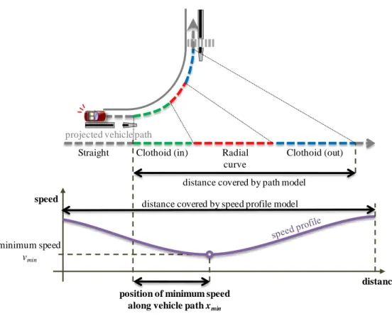
The speed profile is related to the intersection indirectly by relating it to the path of the vehicle. The distance between the beginning of the turning path of the vehicle as described in Section 2.2 and the position where the vehicle reaches its minimum speed is empirically modeled as a random distribution. In this way the path, the speed profile and the intersection geometry are connected to each other (Figure 2.8).

2.4 Stop-go decision at the onset of yellow

When drivers approach an intersection and they observed the signal change from green to yellow, they need to make a decision either to stop or to go through the intersection. Drivers’ stop-go decision is a function of several parameters such as time to stop line at the onset of yellow, all-red interval, vehicle speed and vehicle type. In this study, the probability that a vehicle will stop is modeled using a Logit model as shown in Equation (2.6).

(2.6)

Where Pstop is the probability to stop at the onset of yellow and Vstop is stopping utility function. For

detailed information about model assumptions and estimation refer to the first year report of the project. Curb radius Intersection angle Entering speed lateral distance at exit Hard nose distance c1,in c1,out vmin xmin ) , ( ) , ( β s m α N G Constraints a_enter , v_enter aexit,vexit

(16)

11

2.5 Drivers acceptance to gaps between pedestrians

Gap is the time difference between two subjects arriving at the same position. In the vehicle-pedestrian conflicts, the available gaps between vehicle-pedestrians for drivers are defined as the time difference between two pedestrians arriving at the conflict point. These gaps are opportunities for drivers to cross. If no suitable gap is available when the vehicle will reach the crosswalk, the driver has to adjust the speed, if necessary to a full stop. The driver will then have to wait until an acceptable gap appears or until all pedestrians have cleared the crosswalk. Therefore, whether available gaps will be accepted or rejected is significantly affected by driver behavior. The occurrence of gaps depends on the characteristics of pedestrian movements.

For the purpose of this research, a gap is defined as the time difference between two successive pedestrians passing the conflict point while a lag is defined as the time needed for one pedestrian to reach the conflict point. Pedestrian movements can have their origin at either the near side or the far side of the crosswalk with reference to conflicting vehicles. Near-side pedestrians are those who start crossing from the side of the vehicular traffic that is exiting the intersection while far-side pedestrians are those who start crossing from the side of the incoming vehicular traffic as shown in Figure 2.9. Considering the vehicle size, the gap is the time difference between the first pedestrian crossing the far edge of the vehicle trajectory and the second pedestrian crossing the near edge of

Figure 2.8 Illustration of position of minimum speed with reference to vehicle path

position of minimum speed along vehicle path xmin

distance speed

minimum speed

vmin

Clothoid (in) Radial curve

Clothoid (out) projected vehicle path

Straight

distance covered by path model distance covered by speed profile model

(17)

12

the vehicle trajectory. The lag is the time between the pedestrian crossing the near edge of the vehicle trajectory and the vehicle arriving at the conflict point as shown in Figure 2.9.

Gaps and lags are calculated when the turning vehicle arrives at the near border of the crosswalk. The gaps between pedestrians who crossed the conflict point before the vehicle reaches the crosswalk are defined as the “unavailable gaps” and they are not considered in this research. The gaps/lags which are used by drivers are called “accepted gaps/lags”, while other gaps/lags which are available but not utilized by drivers are called “rejected gaps/lagｓ”.

a) The definition of near-side and far-side pedestrian origin-destination

b) Gap/lag definition

Figure 2.9 Pedestrian origin-destination and gap/lag definition considering vehicle size

Vout Near-side Far-side Far-side F a r-si d e F a r-sid e N ea r-sid e Near-side N ea r-si d e 0 Time Vehicle starts to stop

Vehicle cross the conflict point Accepted gap Rejected gap Time 0 Dis ta nce fr o m the v ehicle to t he co nflic t p o int Dis ta nce fr o m the pedes tria n to t he co nflic t p o int Near-side Far-side

(18)

13

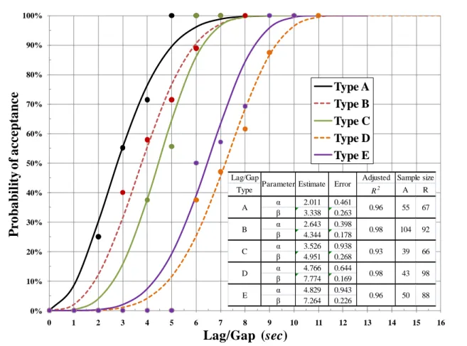
Generally, lags/gaps are classified into five different types depending on the pedestrians’ direction of movement as shown in Figure 2.10.

Type A: lags of pedestrians approaching from the near side of the crosswalk; Type B: lags of pedestrians approaching from the far side of the crosswalk.

Type C: gaps between two pedestrians approaching from the near side of the crosswalk; Type D: gaps between two pedestrians approaching from the far side of the crosswalk;

Type E: gaps between a pedestrian approaching from the near side of the crosswalk and another one approaching from the far side of the crosswalk.

In order to estimate the gap/lag acceptance probability distribution for each type of the defined gaps/lags, empirical data is necessary. After collecting the required data, gaps/lags are categorized into several classes. The gap/lag acceptance probability for class i is calculated according to equation (2.7). gs ed gaps/la of obserev Total No. gs ed gaps/la No. Accept P(x)_i (in category i) (2.7) A Cumulative Weibull Distribution is used to fit the observed gap/lag acceptance probability distributions. The Weibull Distribution is a widely used function to represent the breakdown probability おｎ highways and expressways. It is also widely used to represent various gap acceptance conditions between different travelers in the transportation network. Equation (2.8)

Figure 2.10 Assumed types of gaps/lags Type A

Type B

Type C

Type D

Type E

Lags of pedestrians from the near-side of the crosswalk.

Lags of pedestrians from the Far-side of the crosswalk.

GaPs between two pedestrians approaching from the near-side of the crosswalk.

GAps between two pedestrians approaching from the far-side of the crosswalk.

Gaps betweEn a pedestrian approaching from the near-side of the crosswalk and another one approaching from the far-side of the crosswalk.

Near-side

(19)

14

presents the Cumulative Weibull Distribution function with two parameters; the shape parameter α and the scale parameter β.

         x e x P( ) 1 _(2.8)

(20)

15

3 Angle Collisions between Right-turning and Cross Traffic

3.1 Overview

To represent angle collisions, the behavior of clearing right-turning vehicles and conflicting through traffic need to be well represented inside the simulation environment. The required models to represent angle collisions are summarized in Figure 3.1b). They are divided into models representing the behavior of the clearing right-turning vehicles (stop-go decision and trajectory) and models representing the behavior of the entering through traffic in the cross street (start-up behavior). All of these models have already been developed during the first year of the project, except the speed profile model as part of the trajectory modeling which will be presented in detail here.

3.2 Stop-go behavior at the onset of yellow

As explained in Section 2.3, the probability of drivers to decide to stop when approaching the intersection at the onset of the yellow signal is modeled by using a Logit Model (Equation (2.6)). The stopping utility function is assumed to have a linear form with independent variables as shown in Table 3.1. By using Equation (2.6) and Table 3.1, the stopping probability can be estimated and then the stop-go decision can be assigned randomly. For detailed information about the assumptions behind this stop-go decision model、 refer to the first year report of the project.

a) Conflict between clearing right-turning

vehicles and entering through vehicles

b) Necessary models

Figure 3.1 Required models to represent the conflict between clearing right-turning vehicles and entering through traffic

Space

Conflict point

Y AR R

Start Response Time (SRT)

Time

Late Exit Time (LET) Intergreen Time IG

PET

Maneuver of Clearing Right-turning vehicles

Start-up Behavior of First Entering Through vehicles

Stop-go Decision Model at the Onset of Yellow

Start Response Time Model (SRT)

Turning Path Model

Speed Profile Model

Entering Acceleration Model

Represent the conflict between clearing right-turning vehicles and entering cross through vehicles

(21)

16

3.3 Path of right-turning vehicles

As explained in Section 2.1, the path of turning traffic is modeled by a combination of straight, circular and Euler spiral curves. The estimated models for the curve segments which are shown in Equations (2.1), (2.2) and (2.3) are listed in Table 3.2 and Table 3.3. It was assumed that the entering spiral curve parameter A1 and the exit spiral curve parameter A2 are dependent on the

minimum speed along the turning maneuver. This minimum speed is modeled for both parts of the trajectory estimation: path and speed.

Thus Vmin is modeled assuming Normal Distribution. For detailed information refer to the first year

report of the project.

Table 3.2 Results of estimated Euler spiral parameters for right-turning vehicles

Explanatory variables

Parameter of entering Euler spiral curve A1(m)

Parameters (t-values)

Parameter of exit Euler spiral curve A2 (m) Parameters (t-values)

Const. -8.65(-3.33) 3.63 (1.64)

Minimum speed Vmin(km/h) 0.294 (4.48) 0.287 (3.05)

Distance from IP point to hard nose (m)* DHN_IN 0.172 (6.90) － DHN_OUT － 0.241 (4.84) Modified R2 0.663 0.424 Sample Size 151 * Refer to Figure 2.2.

Table 3.1 Right-turning vehicle stop-go model parameter estimation

Explanatory variable Estimate (t-value) 単純 4 現示制御 Permissive followed by exclusive right-turning phase 矢印制御 Exclusive right-turning phase only Travel time to the stop line at the onset of

yellow (sec) 0.71 (7.33) 0.88 (6.29)

Follower dummy (Follower = 1, Otherwise

= 0)) -1.12 (-2.00) -1.37 (-2.57) Constant -2.25 (-3.56) -3.25 (-4.44) 0.362 0.366 的中率 (%) Hit ratio % 80.7 79.6 Sample size 238 167

(22)

17

3.4 Speed profile of right-turning vehicles

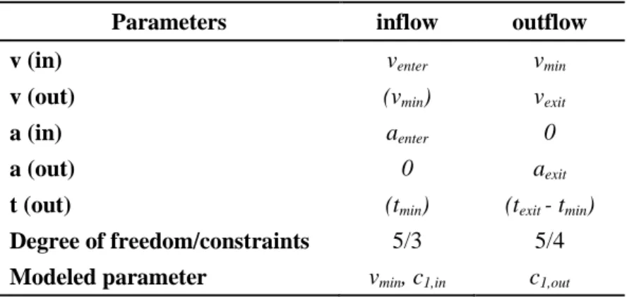
The basic principles of the speed of vehicles when turning at a signalized intersection have been explained in Section 2.3. The particularities of right-turning speed profiles are incorporated into the model by empirical analysis of the speed function coefficients and constraints. Table 3.4 shows the constraints for the speed equation (2.4) with the acceleration as the first derivative and their four unknowns for both the inflow and outflow part of the ideal speed profile (cf. Figure 2.4). This system of linear equations is underdetermined. The coefficient c1 (inflow and outflow) and the

minimum speed vmin are empirically modeled.

Table 3.4 Constraints and modeled parameters for ideal speed profile

Parameters inflow outflow

v (in) venter vmin

v (out) (vmin) vexit

a (in) aenter 0

a (out) 0 aexit

t (out) (tmin) (texit - tmin)

Degree of freedom/constraints 5/3 5/4

Modeled parameter vmin, c1,in c1,out

In addition to vmin, c1,in and c1,out the position of the speed profile with reference to the path of the

vehicle xmin is empirically modeled (cf. Subsection 2.3.4). The observed behavior of vehicles

reveals that these parameters are related to certain intersection characteristics, namely the Table 3.3 Results of estimated minimum radius and minimum speed for right-turning vehicles

time Explanatory variables

Radii of circular curve Rmin (m) Parameters (t-values)

Minimum speed Vmin (km/h) Parameters (t-values)

Average

Const. - 4.49 (2.62)

Intersection angle (deg) 0.0621 (3.80) 0.0717 (5.57)

Distance from IP point to hard nose (m) *

DHN_IN - 0.00920 (4.52)

DHN_OUT - 0.105 (3.17)

Minimum between DHN_IN and

DHN_OUT

0.159 (4.35) -

Minimum speed Vmin(km/h) 0.438 (7.63) 0.380 (13.13)

Standard deviation

Const. - 0.124 (2.69)

Intersection angle (deg) - 1.71 (4.57)

Minimum speed Vmin(km/h) 0.130 (17.4) -

Sample Size 151

(23)

18

intersection angle and the position of the hard nose (cf. Figure 2.2). Correlation charts with the different influencing factors are shown on the following pages. The linear trend is shown with the mean plus/minus the standard deviation indicated by dashed lines.

The parameters are modeled as randomly distributed values. For the coefficients characterizing the random distribution, a linear combination of the most important influencing factors has been used. The coefficients are given in a table for each speed profile parameter.

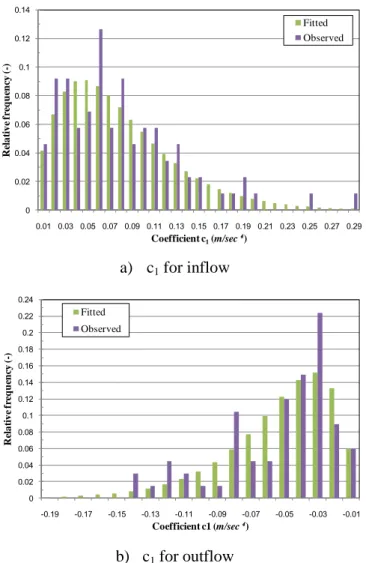
Coefficients c1,in (inflow) and c1,out (outflow)

The coefficient c1 is a jounce parameter (first derivative of the acceleration). It determines the

shape of the speed profile. For the inflow it is positive, for the outflow it is negative. The distribution shows a distinct positive skew. Therefore, a Gamma Distribution was chosen to represent the data as shown in Figure 3.2.

a) c1 for inflow

b) c1 for outflow

Figure 3.2 Modeled and fitted c1 coefficients or the inflow and outflow of right-turning vehicles 0 0.02 0.04 0.06 0.08 0.1 0.12 0.14 0.01 0.03 0.05 0.07 0.09 0.11 0.13 0.15 0.17 0.19 0.21 0.23 0.25 0.27 0.29 R el a ti v e fr eq u en cy ( -) Coefficient c1(m/sec⁴) Fitted Observed 0 0.02 0.04 0.06 0.08 0.1 0.12 0.14 0.16 0.18 0.2 0.22 0.24 -0.19 -0.17 -0.15 -0.13 -0.11 -0.09 -0.07 -0.05 -0.03 -0.01 R el a ti v e fr eq u en cy ( -) Coefficient c1 (m/sec⁴) Fitted Observed

(24)

19

While for the outflow no significant influencing factors on the shape and scale of the Gamma Distribution could be determined, a correlation between the coefficient of the inflow and intersection angle and entering speed can be discerned (Table 3.5).

Minimum speed

The distribution of minimum speeds of right-turning vehicles is symmetric as shown in Figure 3.3 thus a Normal Distribution is used to fit the minimum speed distribution. However, this distribution is affected by different parameters, for instance intersection angle, entering speeds and vehicle type. Since sufficient data to analyze the effect of heavy vehicles is not available, the analysis is limited to approaching speed and intersection angle. Figure 3.4 indicates a linear correlation between the minimum speed and the entering speed and the intersection angle. The two dashed lines stand for the area around the mean with The final model for minimum speed is presented in Table 3.6.

Figure 3.3 The distribution of observed minimum speeds vmin for right-turning vehicles

0% 20% 40% 60% 80% 100% 0 1 2 3 4 5 6 7 8 9 10 0 0 .6 ₁.2 ₁.8 ₂.4 3 3 .6 ₄.2 ₄.8 ₅.4 6 6 .6 ₇.2 ₇.8 ₈.4 9 9 .6 1 0 .2 1 0 .8 1 1 .4 12 1 2 .6 1 3 .2 1 3 .8 F re q u en cy ( -)

Minimum speed (m/sec) Frequency

Cumulative %

Table 3.5 Models of c1,in and c1,out coefficients for right-turning vehicles

Gamma

Distribution Parameters α β

c1,in

α β

c1,out Estimate (Sig.) Estimate (Sig.)

α

Const 9.412827 (0.000) 2.089874 (0.000)

Intersection angle

(degrees) -0.0759988 (0.000) -

Entering speed (m/sec) - -

β

Const -0.0548171 (0.000) .0231397 (0.000)

Intersection angle

(degrees) 0.0007814 (0.000) -

Entering speed (m/sec) 0.0015876 (0.006) -

Log Likelihood

(25)

20 Position of minimum speed xmin on the vehicle path

The position of the minimum speed xmin is defined as the distance from the beginning of the turning

path of the vehicle (first clothoid) of the vehicle path in the intersection to the point where the minimum speed vmin occurs (cf. Subsection 2.3.4). As shown in Figure 3.5 xmin follows a symmetric

distribution; therefore, it is modeled as a Normal Distribution. The final model for xmin is presented

in Table 3.6.

Table 3.6 Minimum speed vmin and position of minimum speed xmin models for right-turning

vehicles Gamma Distribution Parameters vmin N xmin N Estimate (Sig.) Estimate (Sig.)

μ

Const 2.650751 (0.002) 7.34586 (0.222)

Intersection angle (degrees) 0.0289023 (0.000) .0775984 (0.236) Entering speed (m/sec) 0.1879437 (0.000) 0.5006655 (0.113) Distance from IP point to

entering hard nose DHN_IN (m)

- 0.2883846 (0.006)

σ

Const 1.404181 (0.002)

Intersection angle (degrees) -.0053573 (0.311) -0.0350408 (0.394)

Entering speed (m/sec) - -0.5276275 (0.029)

Distance from IP point to entering hard nose DHN_IN (m)

-- 0.110498 (0.059)

Log likelihood -118.95941 -288.69583

Sample Size 87 87

a) Entering speed and Minimum speed b) Intersection angle and Minimum speed Figure 3.4 Correlation between entering speed, intersection angle and minimum speed for

right-turning traffic 0 2 4 6 8 10 12 14 6 8 10 12 14 16 18 20 22 Mi n im u m s p ee d ( m /s ec )

Entering speed (m/sec)

s

m



s

m



0 2 4 6 8 10 12 14 50 60 70 80 90 100 110 120 Mi n im u m s p ee d ( m /s ec )

Intersection angle (degrees)

s

m



s

m



(26)

21

a) Intersection angle and xmin b) Entering speed venter and xmin

c) Distance from IP point to hard nose DHN_OUT and xmin

Figure 3.6 Correlation between several parameters and position of minimum speed xmin for

right-turning vehicles 0 10 20 30 40 50 60 40 60 80 100 120 P o si ti o n o f m in im u m s p e e d xm in (m ) Angle (deg)

s

m



s

m

 0 10 20 30 40 50 60 0 5 10 15 20 25 P o si ti o n o f m in im u m s p e e d xm in (m ) Entering speed (m/s)

s

m



s

m

 0 10 20 30 40 50 60 70 80 0 10 20 30 40 50 P o si ti o n o f m in im u m s p e e d xm in (m )

Distance from IP point to hard nose DHN_OUT (m)

s

m



s

m



Figure 3.5 The distribution of observed xmin (position of minimum speed) for right-turners

0% 10% 20% 30% 40% 50% 60% 70% 80% 90% 100% 0 1 2 3 4 5 6 7 8 9 9 ₁₁ ₁₃ ₁₅ ₁₇ ₁₉ ₂₁ ₂₃ ₂₅ ₂₇ ₂₉ ₃₁ ₃₃ ₃₅ ₃₇ ₃₉ ₄₁ ₄₃ ₄₅ ₄₇ ₄₉ ₅₁ ₅₃ ₅₅ F re q u en cy ( -)

Position of minimum speed xmin(m)

Frequency Cumulative %

(27)

22

3.5 Start-up behavior of through traffic

At intersections with the common lag-lag phasing plan (単純 4 現示制御), it was observed that the clearing behavior of right-turning traffic affects the start-up behavior of the following cross through traffic. Thus, the start-up response time (SRT) of the through traffic is modeled assuming a Weibull Distribution. As shown in Equation (3.1), the Weibull Distribution has three distribution parameters, shape α, scale β, and location γ. Each of them was estimated by influencing factors such as intersection geometry, signal control, and traffic conditions. More specifically, explanatory variables include the distance between the opposite stop-lines, set-back of the stop-line, the entering distance (xSe), late exit time (xLET), length of the all-red time (xAR), signal phasing plan

(dummy variable:the permitted-and-protected right-turn phasing plan or the dual-lagging protected-only right-turn phasing plan), and vehicle type (dummy variable, xheavy: passenger car or heavy

vehicle). Based on statistical tests, the basic structure of the final models is described through Equations (3.1)~(3.4), and the estimated coefficients are presented in Table 3.7.

) ) ( exp( ) ( ) (  1            t  t t f _(3.1) heavy heavy

x

a





0



(3.2) only protected only protected AR AR Se Se

x

b

x

b

x

b



 



₀



(3.3) LET LET

x

c





₀



(3.4)

Where, a0, b0, and c0 are constants; aheavy, bAR, bprotected-only, and cLET are coefficients. The empirically

estimated constants and coefficients are listed in Table 3.7. For detailed information about the estimated start-up response time SRT model refer to the first year report of the project.

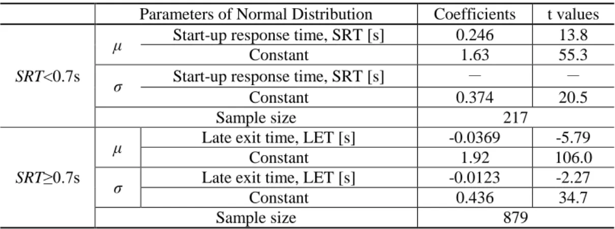
After determining the SRT, it is necessary to estimate the acceleration of the entering through vehicle until it reaches the conflict point. An empirical analysis was conducted to understand the distribution of this acceleration. Finally, as it was reported in the first year report, the entering acceleration is modeled assuming a Normal Distribution. The mean and standard deviation are modeled as a function of explanatory variables as shown in Table 3.8. The SRTs were divided into two populations by taking 0.7s as the threshold value. Both populations are described by Normal Distributions as shown in Table 3.8. The results suggest that hurry-start vehicles adjust their acceleration rates based on the onset time of green, while the other vehicles adjust their acceleration rates according to late exit time LET of the clearing vehicles. For detailed information refer to the first year report of the project.

(28)

23

3.6 Safety Indices

After modeling the clearing behavior of right-turning traffic and the starting behavior of crossing through traffic, the conflict between these two traffic movements can be evaluated and assessed. Various safety indices can be used to quantify these conflicts such as post encroachment time (PET) or time to collision (TTC). In this study, a unique index is proposed for the safety assessment of angle collision between right-turning and cross traffic. The proposed index is called Angle Collisions Index ACI. This index is based on combining two dimensions, the frequency and the potential severity of vehicle-vehicle conflicts.

In past research, the frequency or rate of reported accidents is commonly used for the evaluation of the safety at intersections. When applying such methods, comprehensive historical accident data is necessary comprising at least several years. Therefore, this accident analysis is suitable for long

Table 3.7 Estimated coefficients of the SRT model

Variables Coefficients t values

α

Dummy variable of vehicle type, aheavy

(1: heavy vehicle; 0: otherwise) -3.40 -2.95

Constant a0 11.8 7.33

β

Entering distance bSe [m] -0.0106 -5.49

Dummy variable of signal phasing plan, bprotected-only

(1: the dual-lagging protected-only g right-turn phasing plan; 0: otherwise)

0.274 3.30

Constant b0 13.9 7.65

γ Late exit time, xexit [s] -0.0597 -5.47

Constant c0 11.8 6.56

ρ2

0.56

Sample size 1189

Table 3.8 Estimated parameters of the acceleration model for the entering though vehicles Parameters of Normal Distribution Coefficients t values

SRT<0.7s

μ Start-up response time, SRT [s] 0.246 13.8

Constant 1.63 55.3

σ Start-up response time, SRT [s] －－

Constant 0.374 20.5

Sample size 217

SRT≥0.7s

μ Late exit time, LET [s] -0.0369 -5.79

Constant 1.92 106.0

σ Late exit time, LET [s] -0.0123 -2.27

Constant 0.436 34.7

(29)

24

term a posteriori assessments. Different alternative intersection layouts or signal timing plans cannot be assessed a priori.

In those cases, the traffic conflict technique (TCT) is applicable in which time indices, e.g. post encroachment time (PET), suggested by Allen, et al. (1978) are usually the measures for safety or risk. However, most of them are initially proposed for estimating safety when gap-acceptance or merging maneuver occur during the green intervals. Very few of them have been widely accepted as a safety measure for signal change intervals (intergreen intervals), due to the complicated traffic flow during this interval. For instance, Tang and Nakamura (2008) proposed the PET as a measure for safety performance during intergreen intervals. A PET correspondent to a change of phases is then defined as the elapsed time from when the last clearing vehicle in the previous phase passes the conflict point till when the first entering vehicle released in the subsequent phase arrives there. In this study, PET is used to estimate the number of conflicts. Conflicts are defined as encroachments between two vehicles with a PET of less than t sec.

However, the PET alone cannot assess the safety of angle collisions, for example the impulse of the vehicles involved in the conflict is not considered, although it is a very important factor in determining the severity of a potential accident. Therefore the proposed Angle Collision Index is defined as in Equation (3.5) to incorporate both the frequency and the potential severity of conflicts.

(3.5) Δke is the change in the total kinetic energy before and after the collision. The term is used to weight the conflicts depending on the value of PET. As the PET becomes shorter, the likeliness of the conflict becomes higher.

To estimate the change in kinetic energy Δke, the following assumptions are made:

• The vehicles undergo a perfectly inelastic collision.

• The two vehicles move with the same speed together after the collision. • The friction between the vehicles and the road can be neglected.

• The loss in Energy reflects how much energy is released if the collision occurs. • The system is isolated, where the momentum will be conserved.

Figure 3.7 illustrates the assumed kinetic energy concept after a collision. Since the collision environment is assumed as being isolated, the momentum is conserved along both reference axes as shown in

Figure 3.7c). Thus Equations (3.6) and (3.7) can be derived. By solving these equations, the change in kinetic energy Δke can be estimated as shown in Equation (3.8).

(30)

25

(3.6)

(3.7)

(3.8)

This index will be used as the output of the simulation model for the safety assessment of angle collisions at signalized intersections.

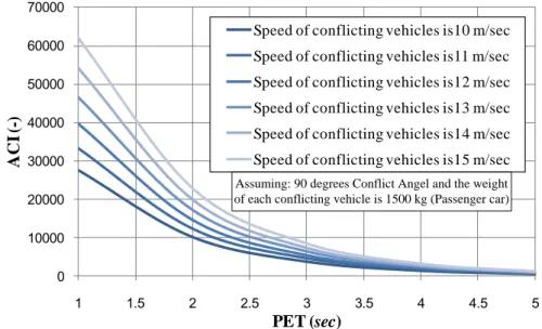
To demonstrate the sensitivity of PCI to PET and conflicting vehicles speed, Figure 3.8 is presented. It assumes a conflict angle of 90 degrees between the two conflicting movement, and a weight of 1500kg for each vehicle with equal speeds. It is rational to see that as PET increases the value of ACI decreases. If PET becomes higher than 5 seconds, the value of ACI becomes negligible. Furthermore at a constant PET, when the speeds of the conflicting vehicles increase,

a) Angle collisions between right-turning

and cross traffic

b) Assumed collision mechanism

c) Momentum analysis along reference axis

Figure 3.7 The estimation of energy loss Δke due to angle collisions

Conflict Area Clearing right-turning vehicle

Entering through vehicle

1  2  2 u 1 u v  Conflict Area 1 1 1usin m 1 1 1ucos m 2 2 2ucos m 2 2 2u sin m  sin ) (m1m2v  cos ) (m1m2v 1



2  2

u

1

u

v



Conflict Area

Where u1 is speed of the clearing right-turning vehicle (m/sec), u2 is the speed of the entering through

vehicle (m/sec), v is speed of clearing right-turning vehicle and entering though vehicle after collision (m/sec), θ1 is the angle between clearing right-turning vehicle and the positive x-axis at the conflict

point (degrees), θ2 is the angle between entering through vehicle and the positive x-axis at the

conflict point (degrees), α is the angle between the collided vehicles and the positive x-axis after collision (degrees), m1 is the mass of the clearing right-turning vehicle (kg) and m2 is the mass of the

(31)

26

ACI increases as shown in Figure 3.8. This is quite rational since it reflects that the severity of a conflict increases as the speed of any of the conflicting vehicles increases.

Figure 3.8 The sensitivity of ACI to PET and the speed of conflicting vehicles 0 10000 20000 30000 40000 50000 60000 70000 1 1.5 2 2.5 3 3.5 4 4.5 5 A C I (-) PET (sec)

Speed of conflicting vehicles is10 m/sec Speed of conflicting vehicles is11 m/sec Speed of conflicting vehicles is12 m/sec Speed of conflicting vehicles is13 m/sec Speed of conflicting vehicles is14 m/sec Speed of conflicting vehicles is15 m/sec

Assuming: 90 degrees Conflict Angel and the weight of each conflicting vehicle is 1500 kg (Passenger car)

(32)

27

4 Left-turning Vehicle Conflicts with Pedestrians

4.1 Overview

Left-turning vehicles are modeled based on four separate models as shown in Figure 4.1. Firstly the behavior of the pedestrians on the crosswalk is analyzed (Section 4.2). Secondly the path of the turning vehicles is modeled (Section 4.4). The vehicles can only pass the crosswalk when sufficient gaps in the pedestrian stream are available. The assessment of the gaps is described in the gap acceptance model (Section 4.3). In addition to the intersection geometry and the driver characteristics, the gap acceptance influences the speed of the vehicles. The speed profile of the turning vehicles is analyzed in Section 4.5. The basic principles of the mentioned models have been described in Chapter 2. Based on these models, conflicts of left-turning vehicles with pedestrians can be assessed by using reasonable safety indices which is discussed in Section 4.6.

4.2 Pedestrian behavior analysis

4.2.1 Methodology

Many factors such as visibility, geometric layout of the intersection, driver behavior while turning and pedestrian behavior influence conflicts between pedestrians and left-turning vehicles. Most of the existing studies which try to analyze the mechanism of such collisions concentrate on driver behavior assuming that it is the most critical factor in determining pedestrian-vehicle collisions. Road users try to anticipate other users’ behavior in order to avoid any collisions with them. Widely varying road user behavior and trajectories may lead to misunderstanding of other users’ decisions which might result in safety problems. Therefore, it is quite important to consider not only vehicles’ maneuver but also pedestrians’ maneuver and its variation which are affected by the

Figure 4.1 Required models to represent the conflict between left-turners and pedestrians

Maneuver of Left-turning

vehicles Pedestrian Behaviour

Gap Acceptance Model

Pedestrian Origin-Destination Model

Turning Path Model

Speed Profile Model

Pedestrian Speed Model

Represent the conflict between left-turning vehicles and crossing pedestrians

(33)

28

geometric layout of intersections, signal timing, and the existence of turning vehicles.

A preliminary macroscopic analysis on pedestrian speed considering the existence of turning vehicles was not successful in finding any significant relationship. Therefore, a microscopic approach is necessary to tackle pedestrian reaction to turning vehicles. Due to the limited time and the complexity of pedestrian maneuver, this study focuses on the effect of pedestrian signal timing and crosswalk geometry upon pedestrian speed at crosswalks as a first step.

In this study, two different spot speeds and two different travel speeds are defined and estimated for each observed pedestrian. Figure 4.2 illustrates the estimated speeds which are defined as follows:

- Entering speed (vin): The spot speed at the entering edge of the crosswalk (m/sec).

- Exit speed (vout): The spot speed at the exit edge of the crosswalk (m/sec).

- First half travel speed (v1): The travel speed in the first half of the crosswalk (m/sec).

- Second half travel speed (v2): The travel speed in the second half of the crosswalk (m/sec).

Figure 4.2 shows how to estimate travel speeds (v1 and v2). Pedestrian origin-destination is defined

as pedestrian movement direction which is divided into two categories; near-side or far-side. One of the reasons behind dividing pedestrians into far-side and near-side is to macroscopically analyze the effect of turning vehicles on pedestrian speed. When comparing v1 and v2, it is important to

remember that the first half of the crosswalk for near-side pedestrians is the second half for far-side pedestrians. In the analysis, pedestrians are also classified into two categories; pedestrians who face

Figure 4.2 Definition of pedestrian spot speeds and travel speeds

f1

f2

f3

f4

Phasing plan at observed intersections

Near-side

Far-side

Position (x1 ,y1)

Timing t1

Entering spot speed vin Position (x2 ,y2)

Timing t2

Position (x3 ,y3)

Timing t3

Exit spot speed vout

Travel speed of the second half of the crosswalk v2

Travel speed of the first half of the crosswalk v1 1 2 2 1 2 2 1 2 1 ) ( ) ( t t y y x x v      2 3 2 2 3 2 2 3 2 ) ( ) ( t t y y x x v     

(34)

29

a turning vehicle while crossing (“with”) and who did not face a turning vehicle (“without”). Pedestrian signal timing is divided into six intervals; R1, G1, G2, G3, PFG and R2 as shown in

Figure 4.3. G1 is defined as 5 s long, assuming that this time in average is enough for the waiting

pedestrians to discharge at the edge of the crosswalk. The second interval G2 is defined based on

the time needed for one pedestrian to cross a half of the crosswalk by assuming a speed of 1 m/sec. In this way G2 is independent of a pedestrian platoon crossing at the same time. The remaining

pedestrian green time is defined as G3. Pedestrians who start crossing before the beginning of

pedestrian green PG are classified as crossing during R1 while those who start crossing after the

end of pedestrian flash green PFG are classified as crossing during R2. R1 is defined as being 10 s,

the remaining pedestrian red time is R2.

v1, v2 and vout for each pedestrian are categorized depending on the entering time to the crosswalk.

For example, if a pedestrian entered the crosswalk in G1, then v1, v2 and vout for that pedestrian will

be classified as crossing during G1.

4.2.2 Data collection and processing

In order to analyze the pedestrian speed at crosswalks, video data was collected at three signalized crosswalks. Table 4.1 presents the observation dates, the geometric and signal timing characteristics of the study sites. All these sites are located in Nagoya City, Japan. The observed crosswalks have significantly different geometric and operational characteristics such as crosswalk

Table 4.1 Surveyed site characteristics

Intersection name Crosswalk position Dimensions w(m)×L(m) Survey hours Cycle Length (sec) Pedestrian green

time PG (sec) Pedestrian flashing green time PFG (sec) PG G1 G2 G3

Imaike East Leg 9m×20m 13:00-15:00 140 35 5 5 25 8

Suemori-Dori2 South Leg 7m×18m 09:00-12:30 140 47 5 4 38 8

Nishi-Osu North Leg 5m×36m 09:00-12:30 160 38 5 13 20 10

G1 G2 G3 5 sec L/2vp PFG PG R1 R2

Figure 4.3 Dividing pedestrian signal timing into several intervals

Where: L is crosswalk length (m), vp is average pedestrian speed (assumed 1m/sec), PG is pedestrian green (sec), PFG is pedestrian flash green (sec), R1 signal interval just before the start of pedestrian green, and R2 is signal interval just after the end of pedestrian flash green.

(35)

30

length and signal timing parameters. All the observed intersections are operated by a 4-phase plan where a shared through-left turning phase is followed by an exclusive right turning phase as shown in Figure 4.2.

The trajectories of pedestrians are extracted from video data by using the image processing system TrafficAnalyzer (Suzuki and Nakamura, 2006). The position of each pedestrian was extracted every 0.5 seconds. The video coordinates were converted to global coordinates. The point where the feet of the pedestrian are touching the ground is the reference observation point. All video observations were done from high buildings around the intersections, thus for all video tapes, the observation angle is large which enables tracking pedestrians without facing any obstacles.

It is important to note that all observed sites have high through traffic demand, thus most of the right turning vehicles turn in their exclusive phase which explains why most of the pedestrian involved in conflicts are with left turning vehicles. Table 4.2 presents the observed number of pedestrians who start crossing in various signal intervals, who face (“with”) or do not face (“without”) turning vehicles, and average left turning vehicle demand (L.T.V). According to observations, the number of pedestrians who start crossing after the end of pedestrian flash green is

Table 4.2 Observed number of pedestrians crossing in different pedestrian signal intervals

Crosswalk Crosswalk position Direction Average L.T.V. demand veh/hr

Observed No. of pedestrians

Total R1 G1

with without with without with without

Imaike East Leg near-side 126 62 200 1 12 4 130

far-side 199 43 9 4 106 27

Suemori-Dori2 South Leg

near-side

312 49 41 0 1 5 35

far-side 59 4 1 0 26 2

Nishi-Osu North Leg near-side 344 172 21 4 11 82 5

far-side 141 2 4 0 73 0

Crosswalk Crosswalk

position Direction

Observed No. of pedestrians

G2 G3 PFG R2

with without with without with without with without

Imaike East Leg near-side 5 37 39 11 13 7 0 3

far-side 27 5 43 6 10 1 4 0

Suemori-Dori2 South Leg

near-side 8 2 33 2 3 1 0 0

far-side 7 1 22 1 3 0 0 0

Nishi-Osu North Leg near-side 64 1 20 4 2 0 0 0

(36)

31

very small while those who start crossing before pedestrian green starts is higher, especially at Imaike Intersection where pedestrian demand is much higher than at other sites.

4.2.3 Analysis of pedestrian speeds

There are several factors that might affect the variations in pedestrian speeds. According to the conducted analysis, signal timing, crosswalk length and the existence of turning vehicles are the most significant factors that affect pedestrian speeds while crossing.

Figure 4.4 shows the mean and the 85 percentile of pedestrians’ entering speeds vin from the

near-side and far-near-side of the crosswalk. It is clear that the average entering speed increases as the time of pedestrian green proceeds. This tendency is understandable, since pedestrians who see the green indication early before reaching the crosswalk tend to hurry up so they can cross before the signal change. This phenomenon is affected by crosswalk length. It is found that both near-side and far-side average pedestrian entering speeds during G3 at Nishiosu intersection are significantly higher (at 95% confidence level) than other sites. Due to the extremely long crosswalk at Nishiosu intersection, pedestrians hurry up when they approach the crosswalk during pedestrian green interval trying to secure as much time as possible for the long crossing distance. This also explains why the differences between the entering speeds in G1, G2 and G3 increase as crosswalk length

Figure 4.4 The mean and 85 percentile of entering speeds vin in different signal intervals

1.44 1.57 1.89 2.70 1.39 1.37 1.72 2.62 1.50 1.74 1.95 1.36 1.39 1.67 1.27 1.72 3.16 1.50 1.58 2.03 1.17 1.34 1.53 1.84 1.06 1.20 1.49 1.97 1.22 1.37 1.56 1.06 1.33 1.48 0.94 1.40 1.96 1.09 1.33 1.62 0.00 0.50 1.00 1.50 2.00 2.50 3.00 3.50 G1 G2 G3 FG G1 G2 G3 FG G1 G2 G3 G1 G2 G3 G1 G2 G3 G1 G2 G3

Near-side Far-side Near-side Far-side Near-side Far-side

Imaike Suemoridori2 Nishiosu

En te ri n g s p ee d vin (m /s ec ) 85 Pecentile Mean ( ) Sample size (134) (42) (50) (26) (133) (32) (49) (19) (40) (10) (35) (28) (8) (23) (87) (65) (24) (73) (46) (13)

効果的な交通安全対策立案のための信号交差点安全性定量評価シュミレーション手法の開発 タカタ財団助成研究論文集 ISSN 2185