Takeshi Otsu
Abstract
In this paper, we examine how a focus on an increase in economic slack
contributes to developing clear quantitative guidelines about how to identify a
recession. We use monthly labor-market indicators of composite indices of Japan.
Firstly, we find that ‘Index of Non-Scheduled Worked Hours(Industries Covered)’ is
a promising variable to identify a recession in Japan. Secondly, the unemployment
rate, found useful to identify the modern U.S. recessions in the literature, does not
produce dates of the turning points consistent with the official reference dates of
Japan.
Key words: economic slack, growth cycles, reference dates JEL classification: E32
1 Introduction
The study of aggregate fluctuations in economy has been a central subject of
economics since the nineteenth century (seePersons, 1926). Burns and Mitchell
(1946)is a compilation of extensive works the NBER researchers undertook at that
time. It has spawned a voluminous literature on the business cycles. One of the key
concepts is the “reference dates,” the dates of peaks and troughs of business cycles.
Burns and Mitchell(1946, pp. 76-77)explained the importance of dating the peaks
and troughs in business-cycle analysis. Romer and Romer(2019)claimed that the
dates played an important role in establishing the concept of a recession as a
starting point of empirical research, but a great concern from the press and
policymakers. Particularly, significant downturns in economic activity are a
fundamental motivating concern.
In the business-cycle literature, it is important to distinguish a classical cycle
and a growth one, as pointed out by Pagan(1997). The classical cycle consists of
peaks and troughs in the levels of aggregate economic activities, often represented
by the gross national product(GDP). On the other hand, the growth cycle exists in
the detrended series, on which the real business-cycle literature focuses. The two
types of cycles show different cyclical timing in general, that is, different dates of
peaks and troughs. When a series has a cyclical component around a deterministic
upward trend, typical as in economic data, detrending would make its cyclical
peaks earlier, while delaying its cyclical troughs(see Bry and Boschan, 1971, p. 11).
The reference dates of the business cycle, officially published in the U.S. and
Japan, conceptually correspond to the timing of peaks and troughs of the classical
cycle. For example, the NBER focuses on peaks and troughs in the level of
economic activity1). The basic dating procedure, widely used in official agencies
and academic researchers, is developed by the National Bureau of Economic
Research (NBER)in the U. S. It applies the Bry-Boschan procedure(see Bry and
Boschan, 1971)to determine turning points of several economic time series selected
as coincident indicators. Dates of these turning points are typically pinned down
by examining a historical diffusion index that shows a share of the number of
series with a positive change, the so-called expanding series. Pagan (1997, p. 3)
argued against detrending transformation of data, because it is not appropriate to
analyze and interpret the growth cycle, citing the business-cycle characteristics
based on the official reference dates.
Fabricant(1972)suggested defining a recession as a decline in the proportion
of available resources employed in production, or as a widening of the gap
between potential and actual output, rather than as a decline in aggregate economic
activity relative to its trend. Following this line, Romer and Romer(2019)proposed
that the NBER should consider replacing its emphasis on a decline in economic
activity with a focus on a large and rapid rise in economic slack, claiming that it
lead to a narrower and more precise definition of a recession that is more firmly
grounded in modern understanding of macroeconomic fluctuations. They showed
some supportive evidence for the United States and Japan in the modern
low-growth era. They argued that it appeared better suited to identifying episodes of
interest in settings where trend growth is low as well as more closely
corresponding to how both economists and the public think of a recession.
In this paper, we examine how a focus on an increase in economic slack
contributes to developing clear quantitative guidelines about how to identify a
recession. We attempt to nail down what variables are useful for analysis of
recessions as well as economic slack. We use labor-market data of Japan that has
recorded a very low rate of economic growth for more than a quarter of century.
We use monthly data of the leading, the coincident, and the lagging indicators,
instead of quarterly data that Romer and Romer (2019) used, to enhance
comparison with the reference dates published in monthly base.
The main findings are as follows. Firstly, ‘Index of Non-Scheduled Worked
Hours(Industries Covered)’ is a promising variable to identify a recession in Japan.
Secondly, the unemployment rate, which Romer and Romer(2019)found useful to
find the modern U. S. recessions, does not produce dates of the turning points
consistent with the official reference dates of Japan.
The rest of the paper is organized as follows. In section 2, we discuss data for
analysis. We use individual indicators of the composite indices, which are related 1) The NBER press release on June 8, 2020: http://www2.nber.org/cycles/june2020.pdf
starting point of empirical research, but a great concern from the press and
policymakers. Particularly, significant downturns in economic activity are a
fundamental motivating concern.
In the business-cycle literature, it is important to distinguish a classical cycle
and a growth one, as pointed out by Pagan(1997). The classical cycle consists of
peaks and troughs in the levels of aggregate economic activities, often represented
by the gross national product(GDP). On the other hand, the growth cycle exists in
the detrended series, on which the real business-cycle literature focuses. The two
types of cycles show different cyclical timing in general, that is, different dates of
peaks and troughs. When a series has a cyclical component around a deterministic
upward trend, typical as in economic data, detrending would make its cyclical
peaks earlier, while delaying its cyclical troughs(see Bry and Boschan, 1971, p. 11).
The reference dates of the business cycle, officially published in the U.S. and
Japan, conceptually correspond to the timing of peaks and troughs of the classical
cycle. For example, the NBER focuses on peaks and troughs in the level of
economic activity1). The basic dating procedure, widely used in official agencies
and academic researchers, is developed by the National Bureau of Economic
Research(NBER)in the U. S. It applies the Bry-Boschan procedure (see Bry and
Boschan, 1971)to determine turning points of several economic time series selected
as coincident indicators. Dates of these turning points are typically pinned down
by examining a historical diffusion index that shows a share of the number of
series with a positive change, the so-called expanding series. Pagan(1997, p. 3)
argued against detrending transformation of data, because it is not appropriate to
analyze and interpret the growth cycle, citing the business-cycle characteristics
based on the official reference dates.
Fabricant(1972)suggested defining a recession as a decline in the proportion
of available resources employed in production, or as a widening of the gap
between potential and actual output, rather than as a decline in aggregate economic
activity relative to its trend. Following this line, Romer and Romer(2019)proposed
that the NBER should consider replacing its emphasis on a decline in economic
activity with a focus on a large and rapid rise in economic slack, claiming that it
lead to a narrower and more precise definition of a recession that is more firmly
grounded in modern understanding of macroeconomic fluctuations. They showed
some supportive evidence for the United States and Japan in the modern
low-growth era. They argued that it appeared better suited to identifying episodes of
interest in settings where trend growth is low as well as more closely
corresponding to how both economists and the public think of a recession.
In this paper, we examine how a focus on an increase in economic slack
contributes to developing clear quantitative guidelines about how to identify a
recession. We attempt to nail down what variables are useful for analysis of
recessions as well as economic slack. We use labor-market data of Japan that has
recorded a very low rate of economic growth for more than a quarter of century.
We use monthly data of the leading, the coincident, and the lagging indicators,
instead of quarterly data that Romer and Romer (2019) used, to enhance
comparison with the reference dates published in monthly base.
The main findings are as follows. Firstly, ‘Index of Non-Scheduled Worked
Hours(Industries Covered)’ is a promising variable to identify a recession in Japan.
Secondly, the unemployment rate, which Romer and Romer(2019)found useful to
find the modern U. S. recessions, does not produce dates of the turning points
consistent with the official reference dates of Japan.
The rest of the paper is organized as follows. In section 2, we discuss data for
analysis. We use individual indicators of the composite indices, which are related 1) The NBER press release on June 8, 2020: http://www2.nber.org/cycles/june2020.pdf
to the labor market in Japan. Section 3 briefly explains the filtering methods used
to estimate economic slack. In section 4, we compare the estimated dates of peaks
and troughs with the official reference dates to investigate whether we can find
economic variables useful for recession identification. The final section is
allocated to discussion.
2 Slack in Labor Market: Data
To measure economic slack, we use time series related to labor market,
included in the composite indices of Japan(see Table 2). The reason to use
labor-market data is that labor labor-market conditions reflect overall economic slack because
all industries use labor. Although capacity utilization ratio can be used, its
coverage is limited to manufacturing, and removed from the individual indicators
of the composite indices in October 2011. Therefore, we focus on the labor-related
variables.
Further, Romer and Romer (2019)found that the unemployment rate was
useful to study a recession in terms of economic slack in the U.S. They argued that
trend growth has been relativelysteady at a moderately positive level for the
modern United States, and that the recessions are all characterized by large and
rapid increases in the unemployment rate. Further, they claimed that a focus on
such a characterization does not alter the chronology of peaks and troughs of the
U. S. business cycles in any important way. It is true, historically, that the
unemployment rate was used extensively to date recessions in the early postwar
period. But, it has played no role in the dating process since it was changed to a
lagging indicator in 1975.
In Japan, the unemployment rate has been introduced as a lagging indicator in
August 1984. Since the growth rate of Japan is less than 1% on average for the last
two decades, a mild shortfall from the growth trend leads to a recession. Therefore,
it is possible for the unemployment rates to characterize recent recessions, and it
would be interesting to reevaluate usefulness of the unemployment in
business-cycle analysis.
A caveat is in order. In January 2018, it was revealed that officials at Ministry
of Health, Labor and Welfare had incorrectly conducted fundamental statistical
survey on labor-related conditions since 2004. Then, in our data set, there are two
indicators that are susceptible to this incorrect compilation. One is ‘Index of
Non-Scheduled Worked Hours’ and the other ‘Index of Regular Workers Employment
(Change from Previous Year).’ According to Economic and Social Research Institute
(ESRI), affiliated with the Cabinet Office, Government of Japan, it has used the
corrected values published by the Monthly Labor Survey since January 2019 for
the time period from January 2012 onward as a remedy for the faulty data problem.
The earlier part of the series than the correction is connected by a link coefficient
method. Such a remedy makes these series good enough for our analysis. Thus, we
use them in the later analysis.
In addition, the reason that we choose labor-related variables from the
individual indicators of composite indices is that they are supposed to have strong
relation with business cycles. ESRI routinely examines and revises the
composition of indicators. The latest revision, the 12th revision, was made in July
2020. All the individual indicators are available since January 1975, amounting to
more than 500 sample points for each series, which would be long enough for our
analysis.
We attempt to estimate economic slack with series discussed above. As
Romer and Romer (2019,see p.12) discussed, a recession can be defined as a
sustained decline in the rate of growth of aggregate economic activity relative to its
long-term trend. Therefore, the ‘slack’ concept is better suited to the growth cycles
to the labor market in Japan. Section 3 briefly explains the filtering methods used
to estimate economic slack. In section 4, we compare the estimated dates of peaks
and troughs with the official reference dates to investigate whether we can find
economic variables useful for recession identification. The final section is
allocated to discussion.
2 Slack in Labor Market: Data
To measure economic slack, we use time series related to labor market,
included in the composite indices of Japan(see Table 2). The reason to use
labor-market data is that labor labor-market conditions reflect overall economic slack because
all industries use labor. Although capacity utilization ratio can be used, its
coverage is limited to manufacturing, and removed from the individual indicators
of the composite indices in October 2011. Therefore, we focus on the labor-related
variables.
Further, Romer and Romer(2019) found that the unemployment rate was
useful to study a recession in terms of economic slack in the U.S. They argued that
trend growth has been relatively steady at a moderately positivelevel forthe
modern United States, and that the recessions are all characterized by large and
rapid increases in the unemployment rate. Further, they claimed that a focus on
such a characterization does not alter the chronology of peaks and troughs of the
U. S. business cycles in any important way. It is true, historically, that the
unemployment rate was used extensively to date recessions in the early postwar
period. But, it has played no role in the dating process since it was changed to a
lagging indicator in 1975.
In Japan, the unemployment rate has been introduced as a lagging indicator in
August 1984. Since the growth rate of Japan is less than 1% on average for the last
two decades, a mild shortfall from the growth trend leads to a recession. Therefore,
it is possible for the unemployment rates to characterize recent recessions, and it
would be interesting to reevaluate usefulness of the unemployment in
business-cycle analysis.
A caveat is in order. In January 2018, it was revealed that officials at Ministry
of Health, Labor and Welfare had incorrectly conducted fundamental statistical
survey on labor-related conditions since 2004. Then, in our data set, there are two
indicators that are susceptible to this incorrect compilation. One is ‘Index of
Non-Scheduled Worked Hours’ and the other ‘Index of Regular Workers Employment
(Change from Previous Year).’ According to Economic and Social Research Institute
(ESRI), affiliated with the Cabinet Office, Government of Japan, it has used the
corrected values published by the Monthly Labor Survey since January 2019 for
the time period from January 2012 onward as a remedy for the faulty data problem.
The earlier part of the series than the correction is connected by a link coefficient
method. Such a remedy makes these series good enough for our analysis. Thus, we
use them in the later analysis.
In addition, the reason that we choose labor-related variables from the
individual indicators of composite indices is that they are supposed to have strong
relation with business cycles. ESRI routinely examines and revises the
composition of indicators. The latest revision, the 12th revision, was made in July
2020. All the individual indicators are available since January 1975, amounting to
more than 500 sample points for each series, which would be long enough for our
analysis.
We attempt to estimate economic slack with series discussed above. As
Romer and Romer (2019, seep. 12) discussed, a recession can be defined as a
sustained decline in the rate of growth of aggregate economic activity relative to its
long-term trend. Therefore, the ‘slack’ concept is better suited to the growth cycles
business cycles because a recession is interpreted as a part of business cycle. We
use bandpass filters to suppress a secular trend and noise components and to
extract detrended growth cycles. Following Burns and Mitchell (1946), the
business cycles are assumed to range from 18 months(1.5 years)to 96 months(8
years), while the secular trend corresponds to the longer-cycle components and the
noise to the shorter ones. The technical details are given in section 3.
We compare dates of turning points in the growth cycles with those of the
reference dates to investigate usefulness of economic slack in identification of a
recession. The reference dates of business cycles in Japan are determined by ESRI
that organizes the Investigation Committee for Business Cycle Indicators to
inspect historical diffusion indexes calculated from selected series of coincident
indexes and other relevant information. Typically, a final decision on turning
points is made about two to three years later. To make a historical diffusion index,
the peaks and troughs of each individual time series are dated by the Bry-Boschan
method. Thus, the reference dates correspond to those of peaks and troughs of the
classical cycles, that is, the Burns-and-Mitchell-type cycle based on the level of
aggregate economic activity. As pointed by Canova(1999, 1994), the dates of peaks
and troughs in the growth cycles deviate from those in the level cycles by two or
three quarters, which is confirmed by Otsu(2013). Therefore, it is expected that a
monthly comparison would show a deviation by 6 to 9 months.
Table 3 shows the reference dates of peaks and troughs identified by ESRI. It
also contains periods of expansion, contraction, and duration of a complete cycle
(trough to trough). There are 15 peak-to-trough phases identified after World War II.
In thesephases, the average period is about 36 monthsfor expansion, 16 for
contraction, and 52 for the complete cycle.
Finally, wealso refer to the composite index of consistent indicators for
judgement on usefulness of the growth cycles to find a recession. The composite
coincident index is complied by ESRI, based on individual consistent indicators on
and after 1980, and available from 1985 onward for the 12th-revision data. In our
analysis, we use the indicators in Table 2 from January 1980 to January 2020 to
enhance comparison with the composite index. All data are obtained from the
website of ESRI2).
3 Departure from Secular Trend: Filtering Methods
In the literature, there are various methods to extract and measure cyclical
information. Canova(2007)gives a concise description of methods frequently used
in macroeconomic analyses. We use bandpass filters to compute departure from
secular trends. They allow us to extract business-cycle components and suppress
secular trends as well as all the cyclical components shorter than and equal to the
seasonal cycles. Therefore, it is possible to obtain detrended components less noisy
as much as possible. The cyclical components, if properly extracted, would
incorporate all the turns to be identified as peaks or troughs of businesss cycles.
We use three types of bandpass filters among others: the
Christiano-Fitzgerald filter(hereafter, CF filter: Christiano and Fitzgerald, 2003), the
Hamming-windowed filter(Iacobucci and Noullez, 2005)and the Butterworth filters(e.g. Gomez,
2001; Pollock, 2000). Note that the sine-based Butterworth filter with the second
order is equivalent to the Hodrick-Prescott (hereafter, HP) filter proposed by
Hodrick and Prescott(1997) (see Gomez, 2001, p. 336).
Canova(1994)examined performance of 11 different detrending methods to
replicate NBER dating, assuming that the detrending removes a secular
component. Similar analyses are conducted by Canova(1999)with 12 methods
including Hamilton (1989)’s procedure. They found that the HP filter and a
2) Indexes of Business Conditions: https://www.esri.cao.go.jp/en/stat/di/di-e.html, Dec. 23, 2020.
business cycles because a recession is interpreted as a part of business cycle. We
use bandpass filters to suppress a secular trendand noise components and to
extract detrended growth cycles. Following Burns and Mitchell (1946), the
business cycles are assumed to range from 18 months(1.5 years)to 96 months(8
years), while the secular trend corresponds to the longer-cycle components and the
noise to the shorter ones. The technical details are given in section 3.
We compare dates of turning points in the growth cycles with those of the
reference dates to investigate usefulness of economic slack in identification of a
recession. The reference dates of business cycles in Japan are determined by ESRI
that organizes the Investigation Committee for Business Cycle Indicators to
inspect historical diffusion indexes calculated from selected series of coincident
indexes and other relevant information. Typically, a final decision on turning
points is made about two to three years later. To make a historical diffusion index,
the peaks and troughs of each individual time series are dated by the Bry-Boschan
method. Thus, the reference dates correspond to those of peaks and troughs of the
classical cycles, that is, the Burns-and-Mitchell-type cycle based on the level of
aggregate economic activity. As pointed by Canova(1999, 1994), the dates of peaks
and troughs in the growth cycles deviate from those in the level cycles by two or
three quarters, which is confirmed by Otsu(2013). Therefore, it is expected that a
monthly comparison would show a deviation by 6 to 9 months.
Table 3 shows the reference dates of peaks and troughs identified by ESRI. It
also contains periods of expansion, contraction, and duration of a complete cycle
(trough to trough). There are 15 peak-to-trough phases identified after World War II.
In these phases, the averageperiod is about 36 months for expansion, 16 for
contraction, and 52 for the complete cycle.
Finally, we also refer to the composite index of consistent indicators for
judgement on usefulness of the growth cycles to find a recession. The composite
coincident index is complied by ESRI, based on individual consistent indicators on
and after 1980, and available from 1985 onward for the 12th-revision data. In our
analysis, we use the indicators in Table 2 from January 1980 to January 2020 to
enhance comparison with the composite index. All data are obtained from the
website of ESRI2).
3 Departure from Secular Trend: Filtering Methods
In the literature, there are various methods to extract and measure cyclical
information. Canova(2007)gives a concise description of methods frequently used
in macroeconomic analyses. We use bandpass filters to compute departure from
secular trends. They allow us to extract business-cycle components and suppress
secular trends as well as all the cyclical components shorter than and equal to the
seasonal cycles. Therefore, it is possible to obtain detrended components less noisy
as much as possible. The cyclical components, if properly extracted, would
incorporate all the turns to be identified as peaks or troughs of businesss cycles.
We use three types of bandpass filters among others: the
Christiano-Fitzgerald filter(hereafter, CF filter: Christiano and Fitzgerald, 2003), the
Hamming-windowed filter(Iacobucci and Noullez, 2005)and the Butterworth filters(e.g. Gomez,
2001; Pollock, 2000). Note that the sine-based Butterworth filter with the second
order is equivalent to the Hodrick-Prescott (hereafter, HP) filter proposed by
Hodrick and Prescott(1997) (see Gomez, 2001, p. 336).
Canova(1994)examined performance of 11 different detrending methods to
replicate NBER dating, assuming that the detrending removes a secular
component. Similar analyses are conducted by Canova (1999)with 12 methods
including Hamilton (1989)’s procedure. They found that the HP filter and a
2) Indexes of Business Conditions: https://www.esri.cao.go.jp/en/stat/di/di-e.html, Dec. 23, 2020.
frequency domain filter as an approximation to the Butterworth filter(see Canova,
1998, p. 483)would be the most reliable tools to reproduce the NBER dates. Otsu
(2013) conducted a comparative analysis among bandpass filters such as the
Christiano-Fitzgerald filter (Christiano and Fitzgerald, 2003), the
Hamming-windowed filter(Iacobucci and Noullez, 2005)and the Butterworth filters(e.g. Gomez,
2001; Pollock, 2000), using Japanese real GDP data. It showed that the Butterworth
filters give the business-cycle dates closest to the official reference dates.
Now we review properties of the three filters in turn: Christiano-Fitzgerald
filter, Hamming-windowed filter, and Butterworth filters. To begin with, we
consider the following orthogonal decomposition of the observed seriesx: x=y+x
〜
(1)
whereyis a signal whose frequencies belong to the interval
{[−b, −a]∪[a, b]}∈[−π, π], whilex〜has the complementary frequencies. Suppose that we wish to extract the signaly. The Wiener-Kolmogorov theory of signal extraction, as expounded by Whittle(1983, Chapter 3 and 6), indicatesycan be written as: y=B(L)x (2) B(L)=
BL,Lx≡x (3)In polar form, we have
B(e)=
1, for ω ∈[−b, −a]∪[a, b]0, otherwise (4)
where0≦a≦b≦π. In the business-cycle literature, the values ofa and b are often set to the frequencies that correspond to 8 and 1.5 years, respectively. In case
of monthly data we use later, the frequency range is set to
2π 96,2π 18
.Theoretically, we need an infinite number of observations,x’s, to compute y. In practice, the filtering methods approximateybyy, a filtered series with a finite filter. To estimateybyy, the Christiano-Fitzgerald filtering is performed in the time domain with truncation at both ends of the sample, while other filtering
methods in the frequency domain are implemented under the circularity
assumption.
Since details of the CF filter and the Hamming-windowed filter are given in
Christiano and Fitzgerald (2003)and in Iacobucci and Noullez (2005), we only
briefly review them. As for Butterworth filters, we describe them in a little detail.
Then, we discuss detrending and boundary treatment.
3.1 Christiano-Fitzgerald Filter
Christiano and Fitzgerald(2003)sought an optimal linear approximation with
finite sample observations. They solved a minimization problem basedon the
mean square error(MSE)criterion in the frequency domain: minimization of a
weighted sum of differences between the ideal bandpass-filter’s weights and their
approximates, using a spectral density of observations as a weight. They derived
optimal filter weights, assuming a difference-stationary process of observed data
with a trend or a drift removed if any.
In their empirical investigations, they examined the effects of the
time-varying weights, the asymmetry, and the assumption on the stochastic process.
They compared variance ratios and correlations between the components extracted
by the Christiano-Fitzgerald filters and the theoretical components based on the
data generating process of observations. To evaluate the second moments of the
theoretical components, they used the Riemann sum in the frequency domain.
They found that the time-varying weights and the asymmetry of the filter
frequency domain filter as an approximation to the Butterworth filter(see Canova,
1998, p. 483)would be the most reliable tools to reproduce the NBER dates. Otsu
(2013) conducted a comparative analysis among bandpass filters such as the
Christiano-Fitzgerald filter (Christiano and Fitzgerald, 2003), the
Hamming-windowed filter(Iacobucci and Noullez, 2005)and the Butterworth filters(e.g. Gomez,
2001; Pollock, 2000), using Japanese real GDP data. It showed that the Butterworth
filters give the business-cycle dates closest to the official reference dates.
Now we review properties of the three filters in turn: Christiano-Fitzgerald
filter, Hamming-windowed filter, and Butterworth filters. To begin with, we
consider the following orthogonal decomposition of the observed seriesx: x=y+x
〜
(1)
whereyis a signal whose frequencies belong to the interval
{[−b, −a]∪[a, b]}∈[−π, π], whilex〜has the complementary frequencies. Suppose that we wish to extract the signaly. The Wiener-Kolmogorov theory of signal extraction, as expounded by Whittle(1983, Chapter 3 and 6), indicatesycan be written as: y=B(L)x (2) B(L)=
BL,Lx≡x (3)In polar form, we have
B(e)=
1, for ω ∈[−b, −a]∪[a, b]0, otherwise (4)
where0≦a≦b≦π. In the business-cycle literature, the values ofa and b are often set to the frequencies that correspond to 8 and 1.5 years, respectively. In case
of monthly data we use later, the frequency range is set to
2π 96,2π 18
.Theoretically, we need an infinite number of observations,x’s, to compute y. In practice, the filtering methods approximateybyy, a filtered series with a finite filter. To estimateybyy, the Christiano-Fitzgerald filtering is performed in the time domain with truncation at both ends of the sample, while other filtering
methods in the frequency domain are implemented under the circularity
assumption.
Since details of the CF filter and the Hamming-windowed filter are given in
Christiano and Fitzgerald (2003) and in Iacobucci and Noullez (2005), we only
briefly review them. As for Butterworth filters, we describe them in a little detail.
Then, we discuss detrending and boundary treatment.
3.1 Christiano-Fitzgerald Filter
Christiano and Fitzgerald(2003)sought an optimal linear approximation with
finite sample observations. They solved a minimization problembased on the
mean square error(MSE) criterion in the frequency domain: minimization of a
weighted sum of differences between the ideal bandpass-filter’s weights and their
approximates, using a spectral density of observations as a weight. They derived
optimal filter weights, assuming a difference-stationary process of observed data
with a trend or a drift removed if any.
In their empirical investigations, they examined the effects of the
time-varying weights, the asymmetry, and the assumption on the stochastic process.
They compared variance ratios and correlations between the components extracted
by the Christiano-Fitzgerald filters and the theoretical components based on the
data generating process of observations. To evaluate the second moments of the
theoretical components, they used the Riemann sum in the frequency domain.
They found that the time-varying weights and the asymmetry of the filter
relatively more important. Further, they claimed that the time-varying weights
should not introduce severe nonstationarity in the filter approximation because the
variance ratios do not vary much through the time. The correlation between the
filtered-out components and the theoretical ones at different leads and lags
symmetrically diminishes as the leads and lags go far away, which might indicate
that the degree of asymmetry was not great. Finally, one of the
Christiano-Fitzgerald filters derived under the Random-Walk data generating process, the
so-called Random Walk filter, gives a good approximation to the optimal filtering that
explicitly used the estimated coefficients of an optimal moving average process
determined empirically. Therefore, they claimed that we could use the Random
Walk filter without inspecting the data generating process even if the random walk
assumption was false.
As argued in Otsu(2015), the cyclical components extracted by CF might be
distorted in magnitude and timing. Its gain function, defined as the modulus of the
frequency response function, shows large ripples over the target ranges, indicating
a large distortion in estimating the cyclical components. The CF filter also shows
leakage effects(see Baxter and King, 1999, p. 580)over higher frequencies of more than 8 periods per cycle. Further, phase shifts are indicated by values of its phase
function, defined as arctangent of the ratio of the real-valued coefficient of the
imaginary part of the frequency response function to the real part value.
3.2 Hamming-Windowed Filter
Iacobucci and Noullez(2005)claimed that the Hamming-windowed filter be a
good candidate for extracting frequency-defined components. The proposed filter
has a flatter response over the passband than other filters in the literature, such as
the HP filter(Hodrick and Prescott, 1997), the BK filter(Baxter and King, 1999), and
the CF filter. This means that it has no exacerbation(see Baxter and King, 1999, p.
580)and eliminates high-frequency components better than the other three filters.
The Hamming-windowed filtering is implemented in the frequency domain.
The procedure is described as follows. First, we subtract, if necessary, the
least-square regression line to detrend the observation series to make it suitable for the
Fourier transform. Second, we implement the Fourier transform of the detrended
series, Third, we convolve the ideal response with a spectral window to find the
windowed filter response in the frequency domain. The window is the so-called
Tukey-Hamming window(Priestly, 1981, pp. 433-442).
3.3 Butterworth Filters
Pollock(2000)has proposed the tangent-based Butterworth filters in the
two-sided expression, which are called rational square-wave filters. The one-sided
Butterworth filters are widely used in electrical engineering, and well documented
in standard text books, such as Oppenheim and Schafer(1999)and Proakis and
Manolakis(2007). The two-sided version guarantees phase neutrality or no phase
shift. It has finite coefficients, and its frequency response is maximally flat over
the pass band: the first(2n−1)derivatives of the frequency response are zero at zero frequency for thenth-order filter. The filter could stationarize an integrated process of order up to2n. The order of the filter can be determined so that the edge frequencies of the pass band and/or the stop band are aligned to some designated
frequencies. Further, Gomez(2001) pointed out that the two-sided Butterworth
filters could be interpreted as a class of statistical models called UCARIMA(the
unobserved components autoregressive-integrated moving average)in Harvey(1989, p.
74). Since the two-sided Butterworth filters are not so often used in the literature,
we present relevant equations to look at them a little bit more closely.
relatively more important. Further, they claimed that the time-varying weights
should not introduce severe nonstationarity in the filter approximation because the
variance ratios do not vary much through the time. The correlation between the
filtered-out components and the theoretical ones at different leads and lags
symmetrically diminishes as the leads and lags go far away, which might indicate
that the degree of asymmetry was not great. Finally, one of the
Christiano-Fitzgerald filters derived under the Random-Walk data generating process, the
so-called Random Walk filter, gives a good approximation to the optimal filtering that
explicitly used the estimated coefficients of an optimal moving average process
determined empirically. Therefore, they claimed that we could use the Random
Walk filter without inspecting the data generating process even if the random walk
assumption was false.
As argued in Otsu(2015), the cyclical components extracted by CF might be
distorted in magnitude and timing. Its gain function, defined as the modulus of the
frequency response function, shows large ripples over the target ranges, indicating
a large distortion in estimating the cyclical components. The CF filter also shows
leakage effects(see Baxter and King, 1999, p. 580)over higher frequencies of more than 8 periods per cycle. Further, phase shifts are indicated by values of its phase
function, defined as arctangent of the ratio of the real-valued coefficient of the
imaginary part of the frequency response function to the real part value.
3.2 Hamming-Windowed Filter
Iacobucci and Noullez(2005)claimed that the Hamming-windowed filter be a
good candidate for extracting frequency-defined components. The proposed filter
has a flatter response over the passband than other filters in the literature, such as
the HP filter(Hodrick and Prescott, 1997), the BK filter(Baxter and King, 1999), and
the CF filter. This means that it has no exacerbation(see Baxter and King, 1999, p.
580)and eliminates high-frequency components better than the other three filters.
The Hamming-windowed filtering is implemented in the frequency domain.
The procedure is described as follows. First, we subtract, if necessary, the
least-square regression line to detrend the observation series to make it suitable for the
Fourier transform. Second, we implement the Fourier transform of the detrended
series, Third, we convolve the ideal response with a spectral window to find the
windowed filter response in the frequency domain. The window is the so-called
Tukey-Hamming window(Priestly, 1981, pp. 433-442).
3.3 Butterworth Filters
Pollock(2000)has proposed the tangent-based Butterworth filters in the
two-sided expression, which are called rational square-wave filters. The one-sided
Butterworth filters are widely used in electrical engineering, and well documented
in standard text books, such as Oppenheim and Schafer(1999)and Proakis and
Manolakis(2007). The two-sided version guarantees phase neutrality or no phase
shift. It has finite coefficients, and its frequency response is maximally flat over
the pass band: the first(2n−1)derivatives of the frequency response are zero at zero frequency for thenth-order filter. The filter could stationarize an integrated process of order up to2n. The order of the filter can be determined so that the edge frequencies of the pass band and/or the stop band are aligned to some designated
frequencies. Further, Gomez (2001) pointed out that the two-sided Butterworth
filters could be interpreted as a class of statistical models called UCARIMA(the
unobserved components autoregressive-integrated moving average) in Harvey(1989, p.
74). Since the two-sided Butterworth filters are not so often used in the literature,
we present relevant equations to look at them a little bit more closely.
BFT= (1+L) (1+L) (1+L) (1+L) +λ(1−L) (1−L) (5)
whereLx=x, andLx=x. Similarly, the highpass filter is expressed as BFT= λ(1−L)(1−L) (1+L) (1+L) +λ(1−L) (1−L) (6)
Note BFT+BFT=1, which is the complementary condition discussed by Pollock(2000, p. 321). Here,λ is the so-called smoothing parameter. We observe that the Butterworth highpass filter in eq.(6) can handle nonstationary components
integrated of order2nor less. Letωthe cutoff point at which the gain is equal to 0.5. It is shown
λ={tan(ω/2)}
(7)
To see this, we replace theL by ein eq.(5) to obtain the frequency response function in polar form as
ϕ(e; λ, n)=
1
1+λ(i(1−e)/(1+e)) (8)
= 1
1+λ{tan(ω/2)} (9)
Here, it is easy to see that eq.(7) holds whenϕ(e)=0.5. We also observe in eq.(9) that the first(2n−1)derivatives ofϕ(e)are zero atω=0; thus, this filter is maximally flat. Note that the gain is the modulus of the frequency response
function, and indicates to what degree the filter passes the amplitude of a
component at each frequency. The Butterworth filters considered here are
symmetric and their frequency response functions are non-negative. Therefore, the
gain is equivalent to the frequency response. Then, we can use eq.(9) to specifyω so that the gain at the edge of the pass band is close to one and that of the stop band
close to zero. Let the pass band[0, ω], and the stop band[ω, π], whereωis smaller thanω. As in Gomez(2001, p. 372), we consider the following conditions for some small positive values ofδandδ,
1−δ<ϕ(e, λ, n)≦1 for ω∈[0, ω] (10) 0≦ϕ(e, λ, n)<δ for ω∈[ω, π] (11) That is, we can control leakage and compression(see Baxter and King, 1999, p. 580)
effects with precision specified by the values ofδandδ. These conditions can be written as follows: 1+
tan(ω/2) tan(ω/2)
= 1 1−δ (12) 1+
tan(ω/2) tan(ω/2)
= 1 δ (13)Then, we can solve for the cutoff frequency(ω)and the filter’s order(n), given ω,ω,δandδ. The closer to zeros bothδandδ, the smaller the leakage and the compression effects. If n turns out not an integer, the nearest integer is selected.
The Butterworth filters could be based on the sine function. Instead of eq.(5)
and eq. (6), the lowpass and the highpass filters can be written as follows,
respectively. BFS= 1 1+λ(1−L) (1−L) (14) BFS= λ(1−L)(1−L) 1+λ(1−L) (1−L) (15) where λ={2 sin(ω/2)} (16)
BFT= (1+L) (1+L) (1+L) (1+L) +λ(1−L) (1−L) (5)
whereLx=x, andLx=x. Similarly, the highpass filter is expressed as BFT= λ(1−L)(1−L) (1+L) (1+L) +λ(1−L) (1−L) (6)
Note BFT+BFT=1, which is the complementary condition discussedby Pollock(2000, p. 321). Here,λ is the so-called smoothing parameter. We observe that the Butterworth highpass filter in eq.(6) can handle nonstationary components
integrated of order2nor less. Letωthe cutoff point at which the gain is equal to 0.5. It is shown
λ={tan(ω/2)}
(7)
To see this, we replace theL by ein eq.(5) to obtain the frequency response function in polar form as
ϕ(e; λ, n)=
1
1+λ(i(1−e)/(1+e)) (8)
= 1
1+λ{tan(ω/2)} (9)
Here, it is easy to see that eq.(7) holds whenϕ(e)=0.5. We also observe in eq.(9) that the first(2n−1)derivatives ofϕ(e)are zero atω=0; thus, this filter is maximally flat. Note that the gain is the modulus of the frequency response
function, and indicates to what degree the filter passes the amplitude of a
component at each frequency. The Butterworth filters considered here are
symmetric and their frequency response functions are non-negative. Therefore, the
gain is equivalent to the frequency response. Then, we can use eq.(9) to specifyω so that the gain at the edge of the pass band is close to one and that of the stop band
close to zero. Let the pass band[0, ω], and the stop band[ω, π], whereωis smaller thanω. As in Gomez(2001, p. 372), we consider the following conditions for some small positive values ofδandδ,
1−δ<ϕ(e, λ, n)≦1 for ω∈[0, ω] (10) 0≦ϕ(e, λ, n)<δ for ω∈[ω, π] (11) That is, we can control leakage and compression(see Baxter and King, 1999, p. 580)
effects with precision specified by the values ofδandδ. These conditions can be written as follows: 1+
tan(ω/2) tan(ω/2)
= 1 1−δ (12) 1+
tan(ω/2) tan(ω/2)
= 1 δ (13)Then, we can solve for the cutoff frequency(ω)and the filter’s order(n), given ω,ω,δandδ. The closer to zeros bothδandδ, the smaller the leakage and the compression effects. If n turns out not an integer, the nearest integer is selected.
The Butterworth filters could be based on the sine function. Instead of eq.(5)
and eq. (6), the lowpass and the highpass filters can be written as follows,
respectively. BFS= 1 1+λ(1−L) (1−L) (14) BFS= λ(1−L)(1−L) 1+λ(1−L) (1−L) (15) where λ={2 sin(ω/2)} (16)
These are the so-called sine-based Butterworth filters. Whenn is equal to two, eq. (15) is the HP cyclical filter, derived in King and Rebelo(1993, p. 224). Thus, as
pointed out by Gomez(2001, p. 336), the sine-based Butterworth filter with order
two (n=2)can be viewed as the HP filter. As in the case of the tangent-based one, the cutoff point,ω, can be determined with the following conditions:
1+
sin(ω/2) sin(ω/2)
= 1 1−δ (17) 1+
sin(ω/2) sin(ω/2)
=1 δ (18)We observe that the Butterworth highpass filter in eq. (6) or eq. (15) can
handle nonstationary components integrated of order 2n or less. Thus, the HP filter can stationarize the time series with unit root components up to the fourth
order. Gomez(2001, p. 367)claimed that the BFT would give better approximations
to ideal low-pass filters than the BFS. A simulation study in Otsu(2007)confirmed
it.
In the paper, we apply the Butterworth filters to extraction of components
over a certain band[ω, ω], whereωis smaller thanω. The bandpass filter is obtained as the difference between two highpass filters in eq.(6), or two lowpass
filters in eq.(5) with different values ofλ, as in Baxter and King (1999, p. 578). Suppose a lowpass filter has the pass band[0, ω]and the stop band [ω, π]. Here,ωindicates a frequency at which the cycle is longer by some periods than atωand corresponds toωin eq.(12), whileωcorresponds toωin (13). This lowpass filter has the cutoff frequency ofωand the order ofndetermined in eq. (12) and (13). Letλthe corresponding value ofλ. Similarly, another lowpass filter has the pass band [0, ω] and the stop band [ω, π]. Here, ω indicates a frequency at which the cycle is shorter by some periods than atω. In short, we assume that ω<ω<ω<ω. ω corresponds to ω in (12), and ω
corresponds toωin (13). The filter has the cutoff frequency ofωand the order ofn. Then, the value ofλ is λ. The bandpass filter,BFT(λ, n, λ, n), can be obtained as
BFT(λ
, n, λ, n)=BFT(λ, n)−BFT(λ, n) (19)
The corresponding frequency response is expressed as
h(ω; λ, n, λ, n)=ϕ(e; λ, n)−ϕ(e; λ, n) (20)
We can obtain the bandpass filter for the sine-type,BFS (λ
, n, λ, n), and its frequency response in a similar manner.
Alternatively, we sequentially apply the highpass filter with a lower cutoff
frequency to a series, and then further apply the lowpass filter with a higher cutoff
frequency to the filtered series. Although Pedersen(2001, p. 1096)reported that the
sequential filtering has less distorting effects than use of the linear combination of
the filters, the empirical results in the following sections do not change whether we
use the difference method(the linear combination)or the sequential method. Yet
another method is to convert the lowpass filter to the bandpass filter by the
frequency transformation, described in a standard textbook (e. g. Proakis and
Manolakis, 2007, p. 733), and explicitly obtain the bandpass filter(see Gomez, 2001, p.
371). This filter, however, has only one order parameter, implicitly assumingnis equal ton. But, the values ofnandnare very different in fact(see Otsu, 2015). Therefore, we would not use the transformation method later in the paper. Here,
we use the difference method, because it is easy to control leakage and
compression effects at a specific frequency.
We need specify two parameter values, n and λ, in eq. (5) or eq. (6) to implement the Butterworth filtering. We obtain these values from eqs.(7), (12) and
These are the so-called sine-based Butterworth filters. Whenn is equal to two, eq. (15) is the HP cyclical filter, derived in King and Rebelo(1993, p. 224). Thus, as
pointed out by Gomez(2001, p. 336), the sine-based Butterworth filter with order
two(n=2)can be viewed as the HP filter. As in the case of the tangent-based one, the cutoff point,ω, can be determined with the following conditions:
1+
sin(ω/2) sin(ω/2)
= 1 1−δ (17) 1+
sin(ω/2) sin(ω/2)
= 1 δ (18)We observe that the Butterworth highpass filter in eq. (6) or eq. (15) can
handle nonstationary components integrated of order 2n or less. Thus, the HP filter can stationarize the time series with unit root components up to the fourth
order. Gomez(2001, p. 367)claimed that the BFT would give better approximations
to ideal low-pass filters than the BFS. A simulation study in Otsu(2007)confirmed
it.
In the paper, we apply the Butterworth filters to extraction of components
over a certain band[ω, ω], whereωis smaller thanω. The bandpass filter is obtained as the difference between two highpass filters in eq.(6), or two lowpass
filters in eq.(5) with different values ofλ, as in Baxter and King(1999, p. 578). Suppose a lowpass filter has the pass band[0, ω]and the stop band[ω, π]. Here,ωindicates a frequency at which the cycle is longer by some periods than atωand corresponds toωin eq.(12), whileωcorresponds toωin (13). This lowpass filter has the cutoff frequency ofωand the order ofndetermined in eq. (12) and (13). Letλthe corresponding value ofλ. Similarly, another lowpass filter has the pass band [0, ω] and the stop band [ω, π]. Here, ω indicates a frequency at which the cycle is shorter by some periods than atω. In short, we assume that ω<ω<ω<ω. ω corresponds to ω in (12), and ω
corresponds toωin (13). The filter has the cutoff frequency ofωand the order ofn. Then, the value ofλ is λ. The bandpass filter,BFT(λ, n, λ, n), can be obtained as
BFT(λ
, n, λ, n)=BFT(λ, n)−BFT(λ, n) (19)
The corresponding frequency response is expressed as
h(ω; λ, n, λ, n)=ϕ(e; λ, n)−ϕ(e; λ, n) (20)
We can obtain the bandpass filter for the sine-type,BFS (λ
, n, λ, n), and its frequency response in a similar manner.
Alternatively, we sequentially apply the highpass filter with a lower cutoff
frequency to a series, and then further apply the lowpass filter with a higher cutoff
frequency to the filtered series. Although Pedersen(2001, p. 1096)reported that the
sequential filtering has less distorting effects than use of the linear combination of
the filters, the empirical results in the following sections do not change whether we
use the difference method(the linear combination) or the sequential method. Yet
another method is to convert the lowpass filter to the bandpass filter by the
frequency transformation, described in a standard textbook (e. g. Proakis and
Manolakis, 2007, p. 733), and explicitly obtain the bandpass filter(see Gomez, 2001, p.
371). This filter, however, has only one order parameter, implicitly assumingnis equal ton. But, the values ofnandnare very different in fact(see Otsu, 2015). Therefore, we would not use the transformation method later in the paper. Here,
we use the difference method, because it is easy to control leakage and
compression effects at a specific frequency.
We need specify two parameter values, n and λ, in eq. (5) or eq. (6) to implement the Butterworth filtering. We obtain these values from eqs.(7), (12) and
andδ. We set bothδandδto0.01.
In the paper, we attempt to extract cyclical components with periods per cycle
of 1.5 years to 8 years. In terms of a period per cycle (p), a frequency (ω)is
expressed as 2π
p . Therefore, using the notation in the previous section, the target
band,[ω, ω], is
2π 96,2π
18
in months. Following Otsu(2015), we setω to 2π132 and ω to 2π
12. In this case, the transition bands are
2π 132, 2π 96
and
2π 18, 2π12
, respectively. Settingωtoωin eq.(12) andωtoωin eq.(13), we findnandω.λis obtained from eq.(7). Similarly, we findnandλby setting ωtoωin eq.(12) andωtoωin eq.(13), together with eq.(7). In a similar way, we compute the parameter values of the sine-based Butterworth filter from eq.(16),eq.(17) and eq.(18).
Two remarks are in order. As is always the case, the sine-based filter
commands a higher order than the tangent-based on under the same precision
values ofδandδ. In addition, as already mentioned, the well-known HP filter is viewed as the sine-based Butterworth filter with an order of two. This implies that
the HP filter either does not preserve the precision or requires a very wide
transition band. In the literature, it is pointed out that it might mislead researchers
to false empirical results (Harvey and Jaeger, 1993), or it could generate spurious
business-cycle dynamics(Cogley and Nason, 1995). In the paper, we use the HP filter
for completeness.
Turning to implementation, we can implement the Butter-worth filtering
either in the time domain or in the frequency domain. Following Pollock(2000),
Otsu (2007)implemented it in the time domain, and found that when the cycle
period is longer than seven, the matrix inversion is so inaccurate that it is
impossible to control leakage and compression effects with a certain precision
specified by eq.(12) and eq.(13), or eq.(17) and eq.(18). Further, the filters at the
endpoints of data have no symmetry due to the finite truncation of filters. This
implies that the time-domain implementation introduces phase shifts. Therefore,
we do not choose the time-domain filtering.
Alternatively, we can implement the Butterworth filtering in the frequency
domain. In the frequency-domain filtering, cyclical components are computed via
the inverse discrete Fourier trans-form, using the Fourier-transformed series with
the frequency response function as their weights. In contrast to the time-domain
filtering, the frequency-domain filtering does not introduce any phase shifts, as the
theoretical background of the symmetrical filters dictates. For the
frequency-domain procedures to work well, it is required that a linear trend be removed and
circularity be preserved in the time series, which we discuss next.
3.4 Detending Method
To obtain better estimates of cyclical components, it is desirable to remove a
linear trend in the raw data. The linear regression line, recommended by Iacobucci
and Noullez(2005), is often used for trend removal. As shown by Chan, Hayya,
and Ord(1977)and Nelson and Kang(1981), however, this method can produce
spurious periodicity when the true trend is stochastic. Another widely-used
detrending method is the first difference, which reweighs toward the higher
frequencies and can distort the original periodicity, as pointed out by Baxter and
King(1999), Chan, Hayya, and Ord(1977), and Pedersen(2001).
Otsu(2011)found that the drift-adjusting method employed by Christiano and
Fitzgerald(2003, p. 439)could preserve the shapes of autocorrelation functions and
andδ. We set bothδandδto0.01.
In the paper, we attempt to extract cyclical components with periods per cycle
of 1.5 years to 8 years. In terms of a period per cycle(p), a frequency (ω)is
expressed as 2π
p . Therefore, using the notation in the previous section, the target
band,[ω, ω], is
2π 96,2π
18
in months. Following Otsu(2015), we setωto 2π132 and ω to 2π
12. In this case, the transition bands are
2π 132, 2π 96
and
2π 18, 2π12
, respectively. Settingωtoωin eq.(12) andωtoωin eq.(13), we findnandω.λis obtained from eq.(7). Similarly, we findnandλby setting ωtoωin eq.(12) andωtoωin eq.(13), together with eq.(7). In a similar way, we compute the parameter values of the sine-based Butterworth filter from eq.(16),eq.(17) and eq.(18).
Two remarks are in order. As is always the case, the sine-based filter
commands a higher order than the tangent-based on under the same precision
values ofδandδ. In addition, as already mentioned, the well-known HP filter is viewed as the sine-based Butterworth filter with an order of two. This implies that
the HP filter either does not preserve the precision or requires a very wide
transition band. In the literature, it is pointed out that it might mislead researchers
to false empirical results(Harvey and Jaeger, 1993), or it could generate spurious
business-cycle dynamics(Cogley and Nason, 1995). In the paper, we use the HP filter
for completeness.
Turning to implementation, we can implement the Butter-worth filtering
either in the time domain or in the frequency domain. Following Pollock(2000),
Otsu (2007)implemented it in the time domain, and found that when the cycle
period is longer than seven, the matrix inversion is so inaccurate that it is
impossible to control leakage and compression effects with a certain precision
specified by eq.(12) and eq.(13), or eq.(17) and eq.(18). Further, the filters at the
endpoints of data have no symmetry due to the finite truncation of filters. This
implies that the time-domain implementation introduces phase shifts. Therefore,
we do not choose the time-domain filtering.
Alternatively, we can implement the Butterworth filtering in the frequency
domain. In the frequency-domain filtering, cyclical components are computed via
the inverse discrete Fourier trans-form, using the Fourier-transformed series with
the frequency response function as their weights. In contrast to the time-domain
filtering, the frequency-domain filtering does not introduce any phase shifts, as the
theoretical background of the symmetrical filters dictates. For the
frequency-domain procedures to work well, it is required that a linear trend be removed and
circularity be preserved in the time series, which we discuss next.
3.4 Detending Method
To obtain better estimates of cyclical components, it is desirable to remove a
linear trend in the raw data. The linear regression line, recommended by Iacobucci
and Noullez(2005), is often used for trend removal. As shown by Chan, Hayya,
and Ord(1977)and Nelson and Kang(1981), however, this method can produce
spurious periodicity when the true trend is stochastic. Another widely-used
detrending method is the first difference, which reweighs toward the higher
frequencies and can distort the original periodicity, as pointed out by Baxter and
King(1999), Chan, Hayya, and Ord(1977), and Pedersen(2001).
Otsu(2011)found that the drift-adjusting method employed by Christiano and
Fitzgerald(2003, p. 439)could preserve the shapes of autocorrelation functions and
There-fore, this detrending method would create less distortion. Let the raw series z,t=1, ⋯, T. Then, we compute the drift-adjusted series, x, as follows:
x=z−(t+s) μ (21)
wheres is any integer and μ= z−z
T −1 (22)
Note that the first and the last points are the same values:
x=x=
Tz−z+s(z−z)
T −1 (23)
In Christiano and Fitzgerald(2003, p. 439),s is set to −1. Although Otsu(2011) suggested some elaboration on the choice ofs, it does not affect the results of our subsequent analyses in the paper. Thus, we also sets to −1.
It should be noted that the drift-adjusting procedure in eq.(21) would make
the data suitable for filtering in the frequency domain. Since the discrete Fourier
transform assumes circularity of data, the discrepancy in values at both ends of the
time series could seriouslydistort the frequency-domain filtering.The eq. (23)
implies that this adjustment procedure avoids such a distortionary effect.
3.5 Boundary Treatment
In addition to the detrending method,we make use of another device to
reduce variations of the estimates at ends of the series: extension with a boundary
treatment. As argued by Percival and Walden(2000, p. 140), it might be possible to
reduce the estimates’ variations at endpoints if we make use of the so-called
reflection boundary treatment to extend the series to be filtered. We modify the reflection boundary treatmentso that the series is extended antisymmetrically instead of symmetrically as in the conventional reflecting rule. Let the extended
seriesf,
f=
x if 1≦ j≦T
2x−x if −T+3≦ j≦0
(24)
That is, theT −2 values, folded antisymmetrically about the initial data point, are appended to the beginning of the series. We call this extension rule the
antisymmetric reflection, distinguished from the conventional reflection.
It is possible to append them to the end of the series. The reason to append the
extension at the initial point is that most filters give accurate and stable estimates
over the middle range of the series. When we put the initial point in the middle part
of the extended series, the starting parts of the original series would have estimates
more robust to data revisions or updates than the ending parts. Since the initial data
point indicates the farthest past in the time series, it does not make sense that the
estimate of the initial point is subject to a large revision when additional
observations are obtained in the future. Otsu(2010)observed that it moderately
reduced compression effects of the Butterworth and the Hamming-windowed
filters. We note that this boundary treatment makes the estimates at endpoints
identically zero when a symmetric filter is applied. We filter the extended series, f, and extract the lastT values to obtain the targeted components.
4 Empirical Analysis
4.1 Dating Algorithm
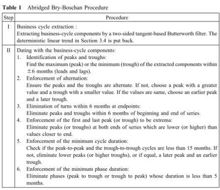
To identify dates of peaks and troughs, we use a modified version of the
Bry-Boschan (BB) method developed by Bry and Boschan (1971). Otsu (2017)
investigated whether the bandpass filtering could simplify the BB algorithm and
found that it would be a good substitute for smoothing procedures involved in the
BB procedure, such as the 12-month moving average, Spencer filtering, and the
There-fore, this detrending method would create less distortion. Let the raw series z,t=1, ⋯, T. Then, we compute the drift-adjusted series, x, as follows:
x=z−(t+s) μ (21)
wheres is any integer and μ= z−z
T −1 (22)
Note that the first and the last points are the same values:
x=x=
Tz−z+s(z−z)
T −1 (23)
In Christiano and Fitzgerald(2003, p. 439),s is set to −1. Although Otsu(2011) suggested some elaboration on the choice ofs, it does not affect the results of our subsequent analyses in the paper. Thus, we also sets to −1.
It should be noted that the drift-adjusting procedure in eq.(21) would make
the data suitable for filtering in the frequency domain. Since the discrete Fourier
transform assumes circularity of data, the discrepancy in values at both ends of the
time seriescould seriously distort the frequency-domainfiltering. The eq. (23)
implies that this adjustment procedure avoids such a distortionary effect.
3.5 Boundary Treatment
In addition to the detrendingmethod, we make use of another device to
reduce variations of the estimates at ends of the series: extension with a boundary
treatment. As argued by Percival and Walden(2000, p. 140), it might be possible to
reduce the estimates’variations at endpoints if we make use of the so-called
reflection boundary treatment to extend the series to be filtered. We modify the reflection boundarytreatment so that the series is extended antisymmetrically instead of symmetrically as in the conventional reflecting rule. Let the extended
seriesf,
f=
x if 1≦ j≦T
2x−x if −T+3≦ j≦0
(24)
That is, theT −2 values, folded antisymmetrically about the initial data point, are appended to the beginning of the series. We call this extension rule the
antisymmetric reflection, distinguished from the conventional reflection.
It is possible to append them to the end of the series. The reason to append the
extension at the initial point is that most filters give accurate and stable estimates
over the middle range of the series. When we put the initial point in the middle part
of the extended series, the starting parts of the original series would have estimates
more robust to data revisions or updates than the ending parts. Since the initial data
point indicates the farthest past in the time series, it does not make sense that the
estimate of the initial point is subject to a large revision when additional
observations are obtained in the future. Otsu (2010)observed that it moderately
reduced compression effects of the Butterworth and the Hamming-windowed
filters. We note that this boundary treatment makes the estimates at endpoints
identically zero when a symmetric filter is applied. We filter the extended series, f, and extract the lastT values to obtain the targeted components.
4 Empirical Analysis
4.1 Dating Algorithm
To identify dates of peaks and troughs, we use a modified version of the
Bry-Boschan (BB) method developed by Bry and Boschan (1971). Otsu (2017)
investigated whether the bandpass filtering could simplify the BB algorithm and
found that it would be a good substitute for smoothing procedures involved in the
BB procedure, such as the 12-month moving average, Spencer filtering, and the