東北大学機関リポジトリTOUR

(1)

Personalized Internal Radiation Dose

Estimation for Nuclear Medicine

著者

MD Shahidul Islam

学位授与機関

Tohoku University

学位授与番号

11301甲第18967号

(2)

Personalized Internal Radiation Dose Estimation for Nuclear Medicine

Md. Shahidul Islam

Graduate School of Biomedical Engineering

Tohoku University, Japan

A thesis submitted to the Graduate School of Biomedical Engineering for the

Degree of Doctor of Philosophy in Biomedical Engineering

(3)

(4)

i

Abstract

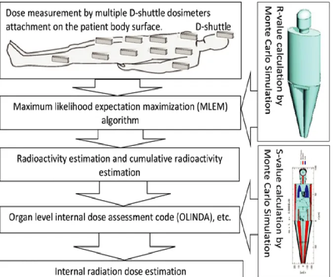
Purpose: Internal radiation dosimetry plays an important role in ensuring the safe use of nuclear medicine technology and is a legal requirement in most countries. Conventionally, the radiation dose is not personalized, which means informed radiation dose to a patient is actually estimated by a rodent data and no consideration of personal information such as age, height, and weight. We propose a new technique to estimate the personalized internal radiation dose in nuclear medicine by means of multiple D-shuttle dosimeters attached on the body surface of the patient.

Methods: Radioactivity in a source organ was estimated iteratively using measurements from multiple D-shuttle dosimeters with a maximum-likelihood expectation-maximization (MLEM) algorithm with dose response from a source to a D-shuttle dosimeter computed by Monte Carlo simulation. We validated the technique in positron emission tomography (PET) study using a National Electrical Manufacturers Association (NEMA) body phantom with 18_F-FDG

solution. The radioactivity concentrations present in the torso cavity and six spheres were 0.00165 MBq/mL and 1.32 MBq/mL, respectively. Eleven D-shuttle dosimeters were attached to the NEMA body phantom surface to obtain information on body surface dose, and a mathematical NEMA body phantom has been modelled in the Heavy Ion Transport Code System (PHITS) Monte Carlo simulation code. To compare the performance of our proposed technique with whole body dynamic PET imaging technique, this phantom was then placed over patient’s bed and imaged for one hour. To investigate the errors associated with the D-shuttle dosimeters positioning on the NEMA body phantom, the mis-locations in a range of 1 to 5 cm at Z-direction (upper) were assumed instead of their original positions. After performing the above-mentioned studies successfully, we performed the several clinical PET studies using 15_{O-water PET radiotracers. Finally, the internal radiation dosimetry was}

estimated through the D-shuttle dosimeter technique in the PET clinical study.

Results: In the validation, a significant correlation (R2 _{= 0.992) was found between actual}

radioactivity and estimated radioactivity at every two-minute interval for the torso cavity and six spheres of NEMA body phantom. In the comparison study, the estimated internal radiation

(5)

Abstract

ii

dosimetry (i.e., cumulative radioactivity, absorbed dose and effective dose) obtained from whole body dynamic PET imagining and D-shuttle dosimeter techniques were very close to the actual radiation dosimetry. The ratios of absorbed doses obtained from D-shuttle and PET measurement against actual were in between 0.9 to 1.3 and 0.7 to 1.0, respectively. The bias for the mis-location of dosimeters were significant. The maximum bias of the average estimated cumulated radioactivity in each compartment and the effective doses were -49.0 % and -71.3 % for the 5 cm shifted positions of all eleven D-shuttle dosimeters, respectively. The most of the estimated dosimetries in clinical PET studies were in agreement with the past studies.

Conclusion: D-shuttle dosimeter technique is capable to conveniently estimate the internal radiation dosimetry successfully in the PET study. Therefore, this technique can be used to evaluate the personalized internal radiation dosimetry routinely in clinical PET study. This method may also be useful for single photon emission computed tomography (SPECT) study, which needs further investigation.

(6)

iii

Acknowledgement

I am sincerely grateful to my supervisor professor, Hiroshi Watabe, for his active guidance, patience, support, cordial encouragement, sincere supervision and whole hearted co-operation throughout my PhD studies without which the completion of the present work would never be done. He did not only help me and guide my research with his advice, but became mentors of mine, to whom I can rely on. I would like to thank professor Manabu Tashiro for supporting me in the PET clinical study and allowing me to work on his projects. I also would like to thank Dr. Miho Shidahara for her advice and comments on my work. I would like to thank Mr. Shoichi Watanuki for supporting me a lot during my experiments. I would also like to thank Mr. Masayasu Miyake for his help, especially in case of dealing with Japanese documentation.

I thank all my lab mates for their advice, comments, participation and support within the lab. I also thank the staffs of Cyclotron and Radioisotope Center (CYRIC) at Tohoku University for their help, especially in case of dealing with academic documentation.

Special acknowledgement to Ministry of Education, Culture, Sports, Science and Technology (MEXT), Japanese Government for giving me the grants to study in Japan.

Finally, I thank my family for their encouragement and continuous support in my life pursue and their company through my tough times in Japan.

(7)

iv

List of Figures

Figure 1. 1: Radiation health effects at different exposure levels………2 Figure 1. 2: Radiation exposure in living environment………7 Figure 1. 3: SHIMADZU Eminence; a modern PET scanner………8 Figure 1. 4: An illustration of the basic biophysics which generates an image utilizing the PET technology………...9 Figure 1. 5: Flowchart of the general imaging procedures for positron emission tomography…9 Figure 1. 6: Concept of the MIRD method. Radiation dose in ith target organ is connected to radioactive decay in each source organ and the so-called S-values from source organ to target organ……….12 Figure 1. 7: Mathematical adult phantom, 1960's version (Snyder et al., 1969) ………15 Figure 1. 8: Anterior view of internal organs of the mathematical adult phantom, 1960’s version (Snyder et al., 1969) ……….………16 Figure 1. 9: Mathematical adult male phantom, 1970's version (Snyder et al., 1978) ………17 Figure 1. 10: Illustration of age-specific mathematical phantoms developed by ORNL………….18 Figure 1. 11: S-value vs body weight for various positron emitting radionuclides; a) Self-absorbed S-value for the kidney, and b) cross Self-absorbed S-value for the kidney irradiating the liver……….………23 Figure 1. 12: Flowchart of the tissue dissection method in animal species for estimating cumulative activity in the human tissue or organ by extrapolating animal data in nuclear medicine……….25 Figure 1. 13: Flowchart of the whole-body PET imaging method for estimating cumulative activity in the interested source organ in nuclear medicine……….………..26 Figure 2. 1: D-shuttle dosimeters which are capable to record every two-minute dose data in the internal memory and can be later read out by a computer interface……….………..33

(13)

List of Figures

x

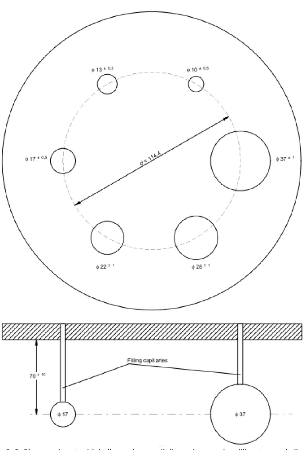
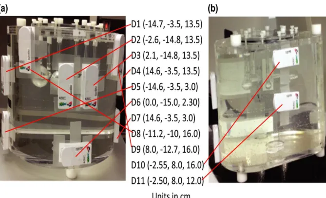
Figure 2. 2: D-shuttle dosimeter with its pocket reader……….……….33 Figure 2. 3: Effective workstation to read out the integrated dose data for calculation and to display the dose graphically for easy comprehension………..………34 Figure 2. 4: Concept of the proposed technique. The body surface dose at the D-shuttle dosimeter position is connected to gamma decay in each source organ and R-values from the source organ to the D-shuttle dosimeter position………..………36 Figure 2. 5: Flowchart of the proposed technique for estimating internal radiation dose in PET studies……….…….38 Figure 3. 1: NEMA body phantom……….………….41 Figure 3. 2: Cross-section of the NEMA body phantom; all dimensions are in millimetres …….41 Figure 3. 3: Phantom insert with hollow spheres; all dimensions are in millimetres and all diameters are inside the diameters……….……….42 Figure 3. 4: Experimental setup and 11 D-shuttle dosimeter (D) positions in Cartesian coordinates on the surface of a NEMA body phantom for obtaining body surface doses; (a) front side of the phantom and (b) back side of the phantom………..………43 Figure 3. 5: Simulated mathematical NEMA body phantom with 11 D-shuttle dosimeter (D) positions in Cartesian coordinates; (a) front side of the phantom and (b) back side of the phantom……….51 Figure 3. 6: (a) Coronal view at Y = 0 cm and (b) lateral view at Z = 13.5 cm of the mathematical NEMA body phantom in PHITS; there are six spheres, with inner diameters of (1) 37 mm, (2) 28 mm, (3) 22 mm, (4) 17 mm, (5) 13 mm, and 6) 10 mm……….……….51 Figure 3. 7: Photon track on XZ plane in PHITS for; a) 10 mm sphere, b) 13 mm sphere, c) 17 mm sphere, d) 22 mm sphere, e) 28 mm sphere, f) 37 mm sphere, and g) torso cavity in mathematical NEMA body phantom……….……..55 Figure 3. 8: Energy spectrum of a) 10 mm sphere, b) 13 mm sphere, c) 17 mm sphere, d) 22 mm sphere, e) 28 mm sphere, f) 37 mm sphere, and g) torso cavity obtained by the Monte Carlo simulation……….59 Figure 3. 9: Correlation between actual radioactivity and estimated radioactivity over 110 min of dose measurements (n = 55) in the source organs……….………..61 Figure 3. 10: Number of iterations vs the cumulative radioactivity in each source organ……...63

(14)

List of Figures

xi

Figure 3. 11: Initial guess vs the cumulative radioactivity in each source organ……….63 Figure 4. 1: Positioning of D-shuttle dosimeters and NEMA body phantom imaging set up as performed in this PET study……….……….71 Figure 4. 2: Super imposed of transmission and emission scans; PET images………..………72 Figure 4. 3: Cumulative radioactivity ratios between the PET and D-shuttle measurements against actual value for all seven source organs (i.e., the torso cavity and six spheres) …...75 Figure 4. 4: Absorbed dose ratios between the PET and D-shuttle measurements against actual value for all seven source organs (i.e., the torso cavity and six spheres). …………..…….…76 Figure 5. 1: D-shuttle dosimeters on the surface of NEMA body phantom; the arrow indicates the centre of mis-located D-shuttle dosimeters at Z direction (upper) in a range of 1 to 5 cm from the original positions (the mis-located D-shuttle dosimeter positions attached the backside of the phantom was not shown) ……….……….80 Figure 5. 2: Mathematical NEMA body phantom in Monte Carlo simulation with accurate and mis-located positions of the D-shuttle dosimeters (D) in the Cartesian co-ordinates; the green and red colors (points) show the accurate positions and the 5 cm shifted positions, respectively……….………..….….81 Figure 5.3: The lateral view at z=13.5 cm of the NEMA body phantom in PHITS; red color represents the position of six spheres in torso, with inner diameters of (1) 37 mm, (2) 28 mm, (3) 22 mm, (4) 17 mm, (5) 13 mm, and 6) 10 mm; x, y, z are 3 dimensional positions and r is the radius of the spheres (units are in cm)………82 Figure 5. 4: Box plots of the bias (%) in the cumulative radioactivity of the torso cavity and six spheres associated with the location of D-shuttle dosimeters; bias due to a) 1 cm location, b) 2 cm location, c) 3 cm location, d) 4 cm location and e ) 5 cm mis-location at z direction upper from the original positions. D1, D1-D2, D1-D3,…., D1-D11 indicate that one (i.e., D1), two (i.e., D1 and D2), three (i.e., D1, D2 and D3),……, eleven (i.e., D1 to D11) D-shuttle dosimeters were mis-located, respectively. Red filled circle represents the average cumulative radioactivity………..………87 Figure 5. 5: Box plots of the bias (%) in the absorbed dose of the torso cavity and six spheres associated with the mis-location of D-shuttle dosimeters; bias due to a) 1 cm mis-location, b) 2 cm mis-location, c) 3 cm mis-location, d) 4 cm mis-location and e ) 5 cm mis-location at z

(15)

List of Figures

xii

direction upper from the original positions. D1, D1-D2, D1-D3,…., D1-D11 indicate that one (i.e., D1), two (i.e., D1 and D2), three (i.e., D1, D2 and D3),……, eleven (i.e., D1 to D11) D-shuttle dosimeters were mis-located, respectively. Red filled circles represent average absorbed doses……….……….90 Figure 6. 1: The 3D view of the Japanese Reference Phantom; a) adult male, and b) adult female……….………..…..98 Figure 6. 2: Coronal view of the principal organs of Japanese reference phantom at; a) Y=0 cm, b) Y= 5 cm, and c) Y=-5cm……….……100 Figure 6. 3: Lateral view of the head and neck portion of the Japanese reference phantom at a) Z= 74.0 cm, b) Z= 73.0 cm, c) Z=69 cm, and d) Z= 64.0 cm……….……102 Figure 6. 4: Lateral view of the trunk portion of the Japanese reference phantom at a) Z= 62.0 cm, b) Z=-52.0 cm, c) Z=-48.0 cm (male), d) Z= 48.0 cm (female), e) Z=44.3 cm, f) Z= 44.0 cm, g) Z=37.0 cm, h) Z= 36.0 cm, i) Z= 30.0 cm, j) Z= 24.0 cm, k) Z=19.0 cm, l) Z=13.0 cm (male), m) Z= 13.0 cm (female), n) Z= 7.0 cm, and o) Z= 4.0 cm………..……….107 Figure 6. 5: Lateral view of the leg portion of the Japanese reference phantom at a) Z= 0.0 cm (male), b) Z=-2.0 cm (male), c) Z=-2.0 cm (female)……….….………108 Figure 6. 6: Skeleton system of Japanese reference phantom in PHITS……….109 Figure 7. 1: A common frame with 14 D-shuttle dosimeters (D2 to D15) to place on the trunk region of the subject for measuring the body surface doses during PET study……….113 Figure 7. 2: Schematic diagram of 15 D-shuttle dosimeters positioning on the subject’s body for detection of body surface doses……….……….114 Figure 7. 3: D-shuttle dosimeter positioning on the torso region of the subject…….………115 Figure 7. 4: D-shuttle dosimeter positioning on the subject’s head……….………115 Figure 7. 5: Japanese reference phantom (JRP) and personalized mathematical Phantom simulated by PHITS; a) (JRP) b) subject-1, b) subject-2, c) subject-3, and d) subject-4….………121 Figure 7. 6: Time-dose curve due to four times bolus injections of [15_{O] water; these body}

surface doses at 2 minutes’ interval were measured by 15 D-shuttle dosimeters (D1 to D15) attachment in the 3rd session of subject-1……….……….122 Figure 7. 7: Time activity curve of nine source organs for bolus injection of [15_{O] water}

(16)

xiii

List of Tables

Table 1.1: The radiation weighting factors for certain types of radiation………..4 Table 1.2: Tissue weighting factor for calculating effective dose (or effective dose equivalent) ………..5 Table 1.3: Positron-emitting radionuclides of interest for biomedical studies………10 Table 1.4: Elemental composition of body tissues in the MIRD phantom expressed as percentage by weight and density of body tissues in [g/cm3]………19 Table 1.5: Organ volume of the ORNL reference phantoms……….………21 Table 1. 6: The height, volume, and weight of the age-specific ORNL phantoms………….……….22 Table 2.1: Specifications of D-shuttle Dosimeter……….35 Table 3. 1: Phantom data for spheres……….….……47 Table 3. 2: Volumes (in ml) of the NEMA body phantom's compartments……….62 Table 3. 3: R-values (mGy/MBq.s) at 11 D-shuttle dosimeter positions (D) for each fillable compartment (treated as source organ) of the NEMA body phantom obtained from the PHITS simulation……….……….60 Table 3. 4: Actual initial radioactivity and estimated initial radioactivity of each fillable compartment (mean with standard deviation, n=55) of the NEMA body phantom [MBq]….…73 Table 4. 1: S-values (mGy/MBq.s) for the torso cavity and six spheres of NEMA body phantom obtained from the Monte Carlo (PHITS) simulation……….….74 Table 4. 2: The actual and estimated cumulative radioactivities [kBq.h/MBq] of the torso cavity and six spheres of the NEMA body phantom……….….74 Table 4. 3: Absorbed dose estimates [mGy/MBq] to target organs and effective dose[mSv/MBq] from 18F-FDG……….….75 Table 5. 1: Number of miss-determined D-shuttle dosimeters and bias (%) in the average cumulative radioactivity of the torso cavity and six spheres and in the effective dose associated with D-shuttle dosimeter positioning on the NEMA body phantom surface……..…84 Table 6. 1: Height and weight of the major sections for representing the Japanese reference phantom……….94

(17)

List of Tables

xiv

Table 6. 2: Organ volume [cm3_{] in Japanese reference phantom (adult male and female) ……95}

Table 6. 3: Elemental composition of body tissues in the Japanese reference phantom (adult male and female) expressed as percentage by weight and density of body tissues in [g/cm3_]

………96 Table 7. 1: D-shuttle dosimeter (D) positions in Cartesian coordinates (X, Y, Z) on the body surface for subject-1………116 Table 7. 2: D-shuttle dosimeter (D) positions in Cartesian coordinates (X, Y, Z) on the body surface for subject-2………116 Table 7. 3: D-shuttle dosimeter (D) positions in Cartesian coordinates (X, Y, Z) on the body surface for subject-3………117 Table 7. 4: D-shuttle dosimeter (D) positions in Cartesian coordinates (X, Y, Z) on the body surface for subject-4………117 Table 7. 5: The injected activity of the tracer [15_{O] water………...118}

Table 7. 6: Outer body dimensions of the four human subjects participated in [15_{O] water PET}

study………119 Table 7. 7: The cumulated activities (±SD) in kBq.h/MBq of nine source organs for each subject for bolus injection of [15_{O] water estimated by D-shuttle dosimeter technique……….124}

Table 7. 8: Comparison of cumulated activities of this work for bolus injection of [15_{O] water}

and other studies due to bolus injection of [15_{O] water or inhalation of [}15_{O] carbon}

dioxide……….……….124 Table 7. 9: Absorbed dose estimates in mGy/MBq (mean ± standard deviation) to various target organs and effective dose in mSv/MBq for each subject from [15_{O] water calculated by}

D-shuttle dosimeter technique……….125 Table 7. 10: Comparison of dosimetry of [15_{O] water in PET study; the dose estimates for}

various organs obtained from D-shuttle dosimeter technique were compared to the past studies reported by ICRP-106, Brihaye et al., Narayana et al., Deloar et al., and Kearfott et al...126

(18)

xv

Abbreviations

AIST National Institute of Advanced Industrial Science and Technology

11_C _Carbon-11

C Carbon

Ca Calcium Cl Chlorine

CYRIC Cyclotron and Radioisotope Center CT Computed Tomography

CV Coefficient of Variation D D-shuttle dosimeter 3D Three-dimensional

DICOM Digital imaging and communications in medicine DNA Deoxyribonucleic acid

EANM European Association of Nuclear Medicine

18_F _Fluorine-18

F Fluorine

Fe Iron

FDG Fluorodeoxyglucose FOV field of view

GPS Global-positioning System

68_Ga _Gallium-68

GSO gadolinium oxyorthosilicate

H Hydrogen

IAEA International Atomic Energy Agency

ICRP International Commission on Radiological Protection

ICRU International Commission on Radiation Units and Measurements IEC International Electrotechnical Commission

JAEA Japan Atomic Energy Agency K Potassium

(19)

Abbreviations

xvi

KEK High Energy Accelerator Research Organization Mg Magnesium

MIRD Medical Internal Radiation Dose

MLEM Maximum-Likelihood Expectation-Maximization MPI Message Passing Interface

MRI Magnetic Resonance Imaging

NEMA National Electrical Manufacturers Association

13_N _Nitrogen-13

N Nitrogen

Na Sodium

NIRS National Institute of Radiological Sciences

15_O _Oxygen-15

O Oxygen

OLINDA Organ Level Internal Dose Assessment ORNL Oak Ridge National Laboratory

P Phosphorus

Pb Lead

PET Positron Emission Tomography PHITS Heavy Ion Transport Code System PMMA polymethylmethacrylate

PVE Partial Volume Effect

82_Rb _Rubidium-82

Rb Rubidium

RCBF Regional cerebral blood flow

RIST Research Organization for Information and Technology

S Sulfur

SAF Specific Absorbed Fraction SD Standard Deviation Si Silicon

(20)

Abbreviations

xvii Sr Strontium

TAC Time Activity Curve

TLD Thermoluminescent Dosimeter VOI volume of interest

Zn Zinc

(21)

xviii

Nomenclature

𝝀 radioactive decay constant [s-1_]

μenρ−1 the mass energy absorption coefficient [m2/kg] 𝝍(𝑬) the photon fluence as a function of energy per unit cumulative

radioactivity in the source organ [1/cm2_/source]

∅_𝒊 the absorbed fraction for radiation I [kg-1_]

∆𝒊 the mean energy of radiation type i [MeV]

𝑨̃ the total cumulative radioactivity in human organ [MBq.h] 𝑨̃_𝒋 the cumulative radioactivity in the jth_{source organ} _[MBq.h]

A(t) the present radioactivity in the source organ [MBq]

𝑨_𝒋(𝒕) the radioactivity at time t in the jth_{source organ} _[MBq]

𝑨𝒋(𝒕)(𝒏) estimated radioactivity at time t at the nth iteration

in the jth_{source organ} _[MBq]

As the activity in source s [MBq]

𝑨̌_𝒔 total number of nuclear transformations in source s [MBq.h]

CV Coefficient of Variation [%]

di(t) the body surface dose at the ith D-shuttle dosimeter

position at time t [mSv]

𝑫̅𝜸(𝒗 ← 𝒔) the mean absorbed dose to volume v in source s [mGy]

𝑫𝒊 radiation dose in the ith target organ [mGy]

DT,R internal radiation dose from radiation R in a tissue or organ T [mGy]

E effective dose [mSv]

HT the equivalent dose in a tissue or organ [mSv]

R the radiation dose at the ith_{D-shuttle dosimeter position per}

unit cumulative radioactivity in the jth_{source organ} _[mGy/MBq.s]

𝑹𝒊,𝒋 the radiation dose at the ith D-shuttle dosimeter position per

unit cumulative radioactivity in the jth_{source organ} _[mGy/MBq.s]

mv the mass of target volume v [kg]

(22)

Nomenclature

xix

𝑺_𝒊,𝒋 the radiation dose in the ith_{target organ per unit}

Cumulative radioactivity in the jth_{source organ} _[mGy/MBq.s]

𝑻𝒌(∞) the body surface dose for infinite time at the k’th TLD position [mSV]

𝑻_𝒌(𝒕_𝟎) the body surface dose at the kth_{TLD position during the}

measuring time period 𝑡0 [mSv]

T1/2 half-life of the radiotracers [s]

WR radiation weighting factor unit less

(23)

1

Chapter 1 Introduction

Nuclear medicine is a medical field to examine and diagnose a patient through radiopharmaceuticals and imaging techniques such as positron emission tomography (PET) and single photon emission computed tomography (SPECT). The nuclear medicine utilizes radioisotope labeled biomolecules, and detection of gamma rays produced by radioactive decay, in order to generate 3D functional images of the body. By altering the radiopharmaceuticals, the nuclear medicine enables to diagnose several diseases such as cancer, heart failure, brain stroke, and dementia. The radioisotopes have long been indispensable in nuclear medicine technology, although ionizing radiation has sufficient energy to affect the atoms in living cells and poses a health risk of the patient.

1.1. The Effects of Radiation

When Ionizing radiation penetrates into the human body, it affects the atoms in living cells and their genetic material (DNA) is damaged. Fortunately, the living cells in the human bodies are extremely efficient to repair most of this damage. If this damage is not repaired correctly, the affected cells may die or eventually become cancerous. The biological effects observed in irradiated persons fall into one of two categories; Deterministic effect and Stochastic effect.

1.1.1. Deterministic effects

Deterministic effects which result in a direct effect, and occurs from radiation-induced cell death at a high enough exposure rate, and can impair the integrity of the organs and tissues in the human body. A threshold dose is needed for damage to become clinically observable, and the extent of damage depends on the absorbed dose, dose rate, and radiation quality.

(24)

Chapter 1: Introduction

2

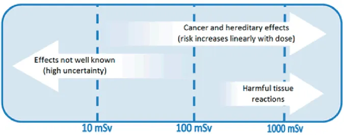
Figure 1. 1: Radiation health effects at different exposure levels (ARPANSA Fact Sheet, 2015)

Thus, the severity of this effect increases with increasing absorbed dose. Early tissue reactions include gastrointestinal symptoms (e.g., haemorrhagic diarrhoea), bone marrow failure (e.g., anaemia and leucocytopenia), skin disturbance (e.g., erythema and epilation), and various other symptoms, and late tissue reactions are cataracts, cardiovascular

disorders, and necrosis. Generally, there will be no direct effect exposure for properly performed diagnostic examinations.

1.1.2. Stochastic effects

Exposure to ionising radiation, even at low doses, can cause damage to the genetic material (DNA) in living cells, which might result in radiation-induced cancer years later, or in heritable disease in the descendants of the exposed individual. These effects are known as stochastic effects of radiation. The probability of the occurrence of the stochastic effect depends on the dose but not severity. The risk of stochastic effects increases with dose, with no threshold.

1.2. Radiation Dose Quantities

The health risk from high radiation doses is relatively well quantified, but for low radiation doses is more limited. While there is a possible increased risk of the stochastic effects at low

(25)

3

radiation doses or for radiation delivered over a long period of time, although these effects are not always detectable. Australian radiation protection and nuclear safety agency has published the following chart for radiation health effect at different exposure levels (Figure 1.1). Therefore, it is essential to evaluate the radiation dose quantities which are described in three ways: absorbed dose, equivalent dose, and effective dose.

1.2.1. Absorbed dose

Absorbed dose describes the intensity of the energy deposited in any small amount of tissue located anywhere in the human body as a result of an exposure to ionizing radiation, and used to assess the potential for biochemical changes in specific tissues. The absorbed dose is measured in a unit called the gray (Gy). A dose of one gray is equivalent to the energy deposited per unit weight (J/kg) at each organ or tissue exposed to radiation. Absorbed dose in a tissue depends on the type of medical examination. For example; the purpose of computed tomography (CT) examination for upper abdomen of a patient, the absorbed dose to the chest is very low, because it has only been exposed to a small amount of scattered radiation. The absorbed dose to the stomach, liver, pancreas and other organs is greatest, because these organs have been directly exposed.

1.2.2. Equivalent dose

When ionizing radiation is absorbed in the tissues or organs or body, a biological effect may be observed. This effect depends on the type of radiation (e.g., alpha, beta, gamma, etc.) and the tissue or organ receiving the radiation. For example, 1 Gy of alpha radiation is more harmful to tissue than 1 Gy of beta radiation. The equivalent dose provides a single unit which accounts for the assessment of harm of different types of radiation. A factor used to equate different types of radiation with different biological effectiveness is called radiation weighting factor (wR). This weighted absorbed quantity is called the equivalent dose. The equivalent

dose is measured in a unit called the sievert (Sv). This means that 1 Sv of alpha radiation will have the same biological effect as 1 Sv of beta radiation. To obtain the equivalent dose, the

(26)

4

absorbed dose is multiplied by the radiation weighting factor (wR). The equivalent dose to a

given tissue or organ is

𝐻𝑇 = ∑ 𝑤𝑅 𝑇

𝐷𝑇,𝑅 (1.1)

Where, DT,R is the internal radiation dose from radiation R in a tissue or organ T, and wR is the

radiation weighting factor. The radiation weighting factors for certain types of radiation as published in International Commission on Radiological Protection (ICRP) 60 are tabulated in Table 1.1.

Table 1. 1: The radiation weighting factors for certain types of radiation.

Type of Radiation Radiation weighting factor

X-rays 1 Gamma rays 1 Beta particles 1 Slow neutrons 5 Fast neutrons 10 Alpha particles 20

1.2.3. Effective dose

Effective dose has been defined and introduced by ICRP for risk management purposes. The effective dose is measured in a unit called the sievert (Sv), and used to assess the potential for long term effects of the patient’s whole body that might occur in future and to compare the stochastic risk of non-uniform exposure to radiation. Since different tissues and organs have different radiation sensitivities, body tissues react differently to radiation and cancer-induction occurs at different rate of dose in different tissues. For example, bone marrow is much more radiosensitive than muscle or nerve tissue. A factor used to equate different types of tissues with different biological effectiveness is called tissue weighting factor (wT).

(27)

5

Table 1. 2: Tissue weighting factor for calculating effective dose (or effective dose equivalent)

Tissue Tissue Weighting Factor

ICRP 26 (1977) ICRP 60 (1990) ICRP 103 (2007)

Bladder 0.05 0.04

Bone marrow (red) 0.12 0.12 0.12

Bone surface 0.03 0.01 0.01 Brain 0.01 Breast 0.15 0.05 0.12 Colon 0.12 0.12 Esophagus 0.05 0.04 Gonads 0.25 0.20 0.08 Liver 0.05 0.04 Lung 0.12 0.12 0.12 Salivary glands 0.01 Skin 0.01 0.01 Stomach 0.12 0.12 Thyroid 0.03 0.05 0.04 Subtotal 0.70 0.95 0.88 Remainder 0.30 0.05 0.12* Total 1.00 1.00 1.00

* ICRP publication 103 remainder tissues include adrenals, extrathoracic (ET) region, gall bladder, heart, kidneys, lymphatic nodes, muscle, oral mucosa, pancreas, prostate, small intestine, spleen, thymus, uterus/cervix.

To obtain an indication of how exposure can affect overall health, the equivalent dose can be multiplied by the tissue weighting factor (wT) related to the risk for a particular tissue or organ.

This multiplication provides the effective dose absorbed by the body. If the body is uniformly irradiated, the summed effective doses are equal to 1. According to ICRP 103, the effective

(28)

6

dose is the sum of the equivalent doses over a defined ensemble of organs each weighted by a tissue weighting factor and expressed by the following formula:

𝐸 = ∑ 𝑤_𝑇 _𝑇𝐻_𝑇 (1.2) Where HT is the equivalent dose in a tissue or organ, wT is the tissue weighting factor. The

tissue weighting factors for calculating effective dose (or effective dose equivalent) are listed in Table 1.2 as published by ICRP.

These factors are normalized in such a way as to ensure that when a person received a uniform gamma exposure, the effective dose in sieverts is equivalent to the absorbed dose in grays. The equivalent doses that are used to calculate the effective doses represent amount of energy deposited per unit of volume in an organ or tissue, and are independent of the size this organ or tissue. If the weighting factors are correctly determined, then valid comparisons can be made between the doses absorbed by people of differing sizes or ages, such as a baby and an adult.

1.3. Radiation Exposure in Living Environment

The National Institute of Radiological Sciences (NIRS), Japan has created a chart of dose scale for radiation exposure in living environment by representing the dose of radiation in milli sievert (mSv) to the entire human body considering sensitivity of each organ or tissue to cancer and hereditary effects (Figure 1.2). In our daily life, we are always exposed to the natural background radiation and artificial radiation. Medical diagnostic tests and treatments are the largest source of artificial (or man-made) radiation exposure in many countries. There is a growing concern over the radiation exposure of a patient due to radiotracer administration during the PET study. Radiation exposure of a patient from a PET scan is modest and depends on the activity of the administrated radiotracer and is typically 8 mSv for adults using 400 MBq of the 18_{F-Fluoro deoxyglucose and is the same whether a part of}

(29)

7

Figure 1. 2: Radiation exposure in living environment (NIRS Report, 2013)

1.4. Positron Emission Tomography (PET) Imaging Technology

Positron emission tomography (PET) is an important radioisotope imaging modality in nuclear medicine for the diagnosis, prognosis, staging, treatment response monitoring, and radiation therapy planning for a wide range of malignancies (Figure 1.3). Nowadays, is has been revolutionary in the diagnosis of cancer.

(30)

8

Figure 1. 3: SHIMADZU Eminence; a modern PET scanner (Shimadzu site)

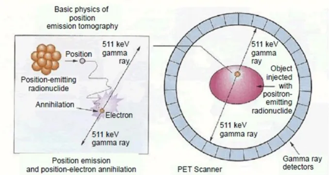
1.4.1. Basic principle

The PET imaging technology utilizes the unique decay characteristics of positron (i.e., an antiparticle to electron with the same mass but with opposite electric charge) emitting radionuclides. A significant amount of radiopharmaceutical synthesized from radionuclide is administered to the patient. When one of the radionuclide atoms decays, a positron is emitted from the nucleus and travels a very short distance in the tissue (typically 10-1_{to 10}0

mm) and annihilates with an electron in the tissue. The annihilation of the particles results in the simultaneous emission of back to back 511 keV gamma rays, as shown in Figure 1.4. The PET systems have sensitive detector panels that register simultaneous gamma hits and their location, thus defining the line alone which the positron emission took place. The three - dimensional functional images of the body reflecting the concentration of the positron-emitting radionuclide can be produced by collecting large numbers of gamma-ray pair events

(31)

9

Figure 1. 4: An illustration of the basic biophysics which generates an image utilizing the PET technology (Jacob et al, 2013).

Figure 1. 5: Flowchart of the general imaging procedures for positron emission tomography

(The electronic text book, University of Calgary Site, 2013-2015) Radionuclide Generation • Cyclotron • Nuclear Reactor • Radionuclide Generator Radiotracer Production • Synthetic biomolecules • Coordination complexes • Salts Radioactive Decay • Positron emission • Annihilation Patient Exposure • Injection • Ingestion Gamma-ray Detection

• Ring of detectors of PET

Image Reconstruction

(32)

10

More sophisticated statistical algorithms are also available to reconstruct the data. Figure 1.4 represents the flowchart of the general imaging procedures for positron emission tomography.

1.4.2. PET- radionuclides and radiotracers

Manmade radionuclides became available for medical use in the late 1930s and the 1940s. These radionuclides are now widely using in the medical science. There are several positron-emitting radionuclides that have been used in PET technology. A list of some commonly used positron-emitting radionuclides and their characteristics appears in Table 1.3.

Table 1. 3: Positron-emitting radionuclides of interest for biomedical studies.

Nuclide Half-life Production Tracer Application

11_C _{20 min} _Cyclotron _Methionine _{Tumour protein synthesis} 13_N _{9.97 min} _Cyclotron _Ammonia _{Myocardial blood flow} 15_O _{122 sec} _Cyclotron _Water _{Cerebral blood flow}

18_F _{110 min} _Cyclotron _FDG _{Glucose metabolism} 68_Ga _{68.1 h} 68_Ge/68_{Ga generator} _DOTANOC _{Neuroendocrine imaging} 82_Rb _{75 sec} _{Reactor, Cyclotron} 82_Rb _{Myocardial perfusion}

1.5. Internal Radiation Dosimetry in Nuclear Medicine

In 1964 and 1965, Ellett et al. performed the Monte Carlo calculations for photon sources of various energies and for target volumes of various sizes and shapes and estimated the absorbed dose to the specific tissues. It was the first application of Monte Carlo methods to radionuclide dosimetry calculations. They formulated an equation and used to internal dosimetry calculations. Their equation for absorbed dose estimation from a gamma ray emitter can be written as follows.

(33)

Chapter 1: Introduction 11 𝐷̅𝛾(𝑣 ← 𝑠) = 𝐴̌𝑠∑ ∆𝑖∅𝑖(𝑣←𝑠) 𝑚𝑣 𝑖 (1.3)

Where 𝐷̅_𝛾(𝑣 ← 𝑠) is the mean absorbed dose to volume v from radioactivity in source s that emits gamma-rays. The symbol As represents the activity in source s, and the symbol

𝐴̌_𝑠 represents the time integral of the activity for the time interval of interest and is called, in medical internal radiation dose (MIRD) terminology, the cumulated activity. Thus, 𝐴̌𝑠

represents the total number of nuclear transformations in source s during the time of interest. The symbol ∆𝑖 represents the mean energy of radiation type i emitted per nuclear

transformation; values of ∆𝑖 are tabulated for various radionuclides in Weber et al. The

symbol ∅𝑖 represents the absorbed fraction for radiation i, and the argument of ∅𝑖 indicates

that it is the fraction of the energy emitted by source s that is absorbed in target volume v. Finally, mv is the mass of target volume v. This equation (1.3) was limited to gamma rays, and

there is no reason why this equation must be limited to gamma rays. Later on, this equation was reformed in general terms by MIRD committee and published in 1968 in the MIRD pamphlet no. 1.

1.6. Medical Internal Radiation Dose (MIRD) Method

In 1965, The Medical Internal Radiation Dose (MIRD) committee was formed by the Society of Nuclear Medicine and charged with the responsibility of providing the nuclear medicine community with guidance on how to calculate the radiation dose from radionuclides. The MIRD facilitates the problem of assessing internal radiation doses by providing models, methodologies, and schema. The internal radiation dosimetry formulation has been adopted by the MIRD computational methodology and simplifies radiation dose calculations for specified target organs from the cumulative radioactivities in source organs and the so-called S-values from the source organ to the target organ (Figure 1.6). Doses due to radioactive decay in source organs are expressed by the following formula:

(34)

12

Figure 1. 6: Concept of the MIRD method. Radiation dose in ith target organ is connected to radioactive decay in each source organ and the so-called S-values from source organ to target organ (Islam et al, 2018).

𝐷_𝑖 = ∑ 𝑆_𝑗 _𝑖,𝑗. 𝐴̃_𝑗. (1.5) Where, 𝐴̃𝑗 is the cumulative radioactivity in the jth source organ, Di is the radiation

dose in the ith target organ, and 𝑆𝑖,𝑗 is the radiation dose in the ith target organ per unit

cumulative radioactivity in the jth source organ. This equation can also be expressed by the following matrix equation:

[ 𝐷₁ 𝐷₂ ⋮ 𝐷𝑖 ] = [ 𝑆_1,1 𝑆_1,2 ⋯ 𝑆1,𝑗 𝑆_2,1 𝑆_2,2 ⋯ 𝑆2,𝑗 ⋮ ⋮ ⋱ ⋮ 𝑆_𝑖,1 𝑆_𝑖,2 ⋯ 𝑆_𝑖,𝑗][ 𝐴̃1 𝐴̃2 ⋮ 𝐴̃_𝑗] (1.6)

(35)

13

The source organs are radioactive, and the target organ is the organ in which the dose is calculated, and the target and source organs can be the same organ. There are few methods for estimating the cumulative radioactivity in the source organ of a patient, and the S-value can be calculated using an MIRD reference phantom and a Monte Carlo simulation. Finally, the radiation dose of the target organ can be estimated from the cumulative radioactivities in the source organs by using computer software, such as the MIRDOSE software, OLINDA/EXM software, SPRIND Software, Hybrid Dosimetry software, etc.

1.7. Monte Carlo Simulation

The Monte Carlo technique was introduced during the 2nd_{World War. Nowadays, it has}

become one of the most important tools in different areas of medical physics following the development and subsequent implementation of powerful computing systems for clinical use. The applications of the Monte Carlo techniques in medical physics cover almost all areas, such as radiation protection, diagnostic radiology, radiotherapy and nuclear medicine, with an increasing interest in exotic and new applications, such as intravascular radiation therapy, and boron neutron capture therapy. In the Monte Carlo technique, the physical systems and phenomena are simulated by statistical methods employing random numbers. The general idea of Monte Carlo method is to form a computerised model, which is as similar as possible to the real physical system, and to create interactions within that system based on known probabilities of occurrence, with random numbers of sampling of the probability. As the number of histories (i.e., individual events) is increased, the quality of the simulated outputs of the system improves, meaning that the statistical relative error decreases. Almost any complex physical system can be modelled in Monte Carlo code. The transport of ionizing radiation particles is simulated by defining a source region with random numbers of particles and a tally with the tracking of the particles; the particles or rays from the source region travels through the system and create the interactions within the system with the random particle numbers and then the particles are traced by the defined tally section to evaluate their trajectories and energy deposition at different points in the system. These interactions determine the penetration and motion of particles. The energy deposited during each

(36)

14

interaction gives the radiation absorbed dose, when divided by the appropriate values of mass. The mean absorbed dose at points of interest can be obtained with acceptable relative errors by performing the Monte Carlo simulation with the sufficient number of interactions. The major issues associated with the Monte Carlo technique include how well the real system of interest can be simulated by a geometrical model, how many histories (i.e. how much computer time) are needed to obtain acceptable relative errors (i.e., uncertainties) (usually around 5%, no more than 10%) and how can measured data be used to validate the theoretical calculations.

1.8. MIRD Reference Phantom

Computerized anthropomorphic mathematical (also called stylised) phantoms can be defined by equation-based analytical functions. For purposes of internal radiation dose calculation, and due to the required computational characteristics, family anthropomorphic mathematical phantoms associated with Monte Carlo simulations have been developed by the Oak Ridge National Laboratory (ORNL), and these phantoms are categorized as MIRD reference phantoms. Mathematical phantoms consist of regularly shaped continuous objects defined by combinations of simple mathematical geometries. Mathematical phantoms have the advantage of being able to model anatomical variability and dynamic organs easily. In the 1960s, the first mathematical phantom representing an adult human in use of Monte Carlo techniques was the development of the Fisher–Snyder heterogeneous, hermaphrodite, anthropomorphic model of the human body to estimate doses from photon emitting radionuclides within organs of the body. This phantom, referred to as ‘MIRD-5 phantom’, was reported in Snyder et al 1969 (see Figure 1.7). They performed the Monte Carlo simulation using three type of tissue densities – skeleton tissue, lung tissue and the bulk soft tissue. This mathematical phantom was developed representing the three principal body sections: an elliptical cylinder for the arms, torso, and hips; a truncated elliptical cone for both the legs and feet; and an elliptical cylinder for the head and neck (See Figure 1.8). In this phantom, the arms are inside the trunk, the legs are not separated from each other, the testes are inside the legs region; and minor appendages (i.e., hands, feet, chin, and nose) are omitted.

(37)

15

(38)

16

Figure 1. 8: Anterior view of internal organs of the mathematical adult phantom, 1960’s version (Snyder et al., 1969).

The simple mathematical geometries such as ellipsoids, elliptical cylinders, and cones were used to represent the internal organs of this phantom. Since these simple equations can only capture the most general description of an internal organ’s position and geometry, the representation of internal organs of this this mathematical phantom is very crude.

In the 1970’s Snyder modified this phantom through separating the legs region into two parts, housing the testes in a male genitalia box between the two legs, and rounding the top of the head. One should note that the reference man was a 20-to-30 years old Caucasian, 70 kg in weight and 174 cm in height. In 1978, Snyder et al reported an improved version of their mathematical phantom which included more than 20 organs and more detailed anatomical

features, and estimated an elaborative set of specific absorbed fraction (SAF) (See Figure 1.9). Organs not seen Adrenals Stomach Marrow Pancreas Skin Spleen Ovaries Testes Thymus Thyroid Uterus Leg bones Brain Skull Spine Arm bone Ribs Lungs Heart Liver Upper large intestine Bladder Kidneys Small Intestine Lower large Intestine Pelvis

(39)

17

Figure 1. 9: Mathematical adult male phantom, 1970's version (Snyder et al., 1978)

70 cm 24 cm

20 cm

80 cm

(40)

18

Figure 1. 10: Illustration of age-specific mathematical phantoms developed by ORNL (Program History, ORNL Site)

In 1987 Cristy and Eckerman of Oak Ridge National Laboratory (ORNL) developed a series of phantoms representing children of different ages, adult male and adult female. The ORNL added analogous phantoms for five pre-adult ages: infant, 1, 5, 10, and 15 years, and one of which (the 15-year-old) also served as a model for the adult female. ORNL's age-specific mathematical phantoms are illustrated in Figure 1.10.

(41)

19

Each ORNL phantom consists of the tissues that are lung tissue, skeleton tissue, and the bulk soft tissue. The different elemental compositions and densities of these tissues are used to perform the Monte Carlo simulation. The three tissues used are composed principally of hydrogen, carbon, nitrogen, and oxygen. The density and the elemental composition of body tissues in these MIRD reference phantoms are tabulated in the Table 1.4.

Table 1. 4: Elemental composition of body tissues in the MIRD phantom expressed as percentage by weight and density of body tissues in [g/cm3].

Element Soft tissue Skeleton Lung Breast

H 10.454 7.337 10.134 11.7 C 22.663 25.475 10.238 38.04 N 2.49 3.057 2.866 0 O 63.525 47.893 75.752 50.26 F 0 0.025 0 0 Na 0.112 0.326 0.184 0 Mg 0.013 0.112 0.007 0 Si 0.03 0.002 0.006 0 P 0.134 5.095 0.08 0 S 0.204 0.173 0.225 0 Cl 0.133 0.143 0.266 0 K 0.208 0.153 0.194 0 Ca 0.024 10.19 0.009 0 Fe 0.005 0.008 0.037 0 Zn 0.003 0.005 0.001 0 Rb 0.001 0.002 0.001 0 Sr 0 0.003 0 0 Zr 0.001 0 0 0 Pb 0 0.001 0 0 Density 1.04 1.4 0.296 0.955

(42)

20

The organ models of these mathematical phantoms are described using some quadric equations; for example, a cylindroid for the torso and two cones for the legs. The equations for the head, trunk, and legs are expressed as follows. The parameters for the x and y axes of the ORNL reference phantoms were adopted from the statistics of Caucasians.

Head: (𝑥 𝐴H) 2 + (𝑦 𝐵H) 2 ≤ 1, 𝐶_T ≤ 𝑧 ≤ 𝐶_T+ 𝐶_H1, (1.7) (𝑥 𝐴H) 2 + (𝑦 𝐵H) 2 + (𝑧−[𝐶T+𝐶H1] 𝐶H2 ) 2 ≤ 1, 𝑎𝑛𝑑 𝑧 ˃ 𝐶_T+ 𝐶_H1 (1.8) Trunk: (𝑥 𝐴T) 2 + (𝑦 𝐵T) 2 ≤ 1, 0 ≤ 𝑧 ≤ 𝐶_T (1.9) Legs: 𝑥2 _{+ 𝑦}2 _{≤ ±𝑥(𝐴} T+ 𝐴T 𝐶L′𝑧), −𝐶L≤ 𝑧 ≤ 0 (1.10)

All equations for boundaries of organs of these ORNL reference phantoms are explicitly defined with realistic sizes. The data of organ volumes were derived from the ICRP publication 23, and these volumes were determined by the organ masses at the various ages. The volume of the principal organs of the age-specific ORNL mathematical phantoms are summarized in Table 1.5. The height, volume, and weight of the age-specific ORNL mathematical phantoms are described in the Table 1.6.

(43)

21

Table 1. 5: Organ volume of the ORNL reference phantoms.

organs

New-born

1 year 5 year 10 year 15 year (Adult female) Adult male Adrenals 5.61 3.39 5.07 6.94 10.1 15.7 Brain 338 850 1210 1310 1350 1370 Gall bladder 2.43 5.50 22.5 44.0 56.0 63.7 Heart Kidneys 22.0 60.5 111 166 238 288 Liver 117 281 562 583 1230 1830 Lung 171 484 980 1530 2200 3380 Stomach 16.37 55.7 119.4 209.8 300 402 Small Intestine 50.9 132 265 447 806 1060 Upper large intestine 20.85 54.3 108.8 183.6 331.2 435.5 Lower large intestine 14.37 37.37 75.11 126.7 227.1 297.9

Kidneys 22 60.5 111 166 238 288 pancreas 2.69 9.87 22.7 28.9 62.4 90.7 Spleen 8.76 24.5 46.4 74.4 119 176 Thymus 10.8 22 28.5 30.2 27.3 20.1 Unary bladder 14.67 39.11 76.2 120.9 188.5 248.7 Leg bones 61.4 207 610 1250 2100 2800 Arm bones 45.3 121 239 404 731 956 Pelvis 28.9 76 151 258 460 606 Spine 50 128 245 403 707 920 Skull 49.8 139 339 434 508 618 Facial skeleton 6013 22.8 114 161 234 305 Rib cage 34 87.4 174 295 531 694 Clavicles 2.62 6.85 13.7 23.2 41.6 54.7 Scapulae 9.64 25.3 50.4 85.7 154 202

(44)

22

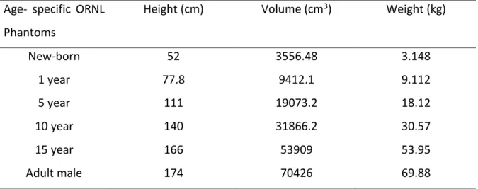
Table 1. 6: The height, volume, and weight of the age-specific ORNL phantoms

Age- specific ORNL Phantoms

Height (cm) Volume (cm3₎ _{Weight (kg)}

New-born 52 3556.48 3.148 1 year 77.8 9412.1 9.112 5 year 111 19073.2 18.12 10 year 140 31866.2 30.57 15 year 166 53909 53.95 Adult male 174 70426 69.88

These age-specific ORNL mathematical phantoms are mainly established using the statistical geometries of Caucasians. The International Atomic Energy Agency (IAEA) reported that the average organ volume of the people of different regions are markedly less than that of Caucasians. The differences in organ mass may exit among the populations from different regions because of their diverse dietary habits, lifestyles, and geographical environments. Therefore, several region-specific reference phantoms are already developed in various regions.

1.9. S-Value

The S-value is the radiation dose in the target organ per unit of cumulative radioactivity in the source organ, which can be calculated using a computerized anthropomorphic phantom and a Monte Carlo simulation. The S-values have a relationship with the body weight of the phantoms. Xie et al reported a relationship between the S-values and body weights of various ages people for various positron emitting radionuclides (see Figure 1.11). The self-absorbed S-values for source organs are contributed from non- penetrating particles (e.g., electrons and positrons), whereas cross-absorbed S-values of different source to target organ pairs are contributed from penetrating radiation.

(45)

23

Figure 1. 11: S-value vs body weight for various positron emitting radionuclides; a) Self-absorbed S-value for kidney, and b) cross Self-absorbed S-value for the kidney irradiating the liver (Xie et al. 2013)

1.10. Cumulative Radioactivity

The cumulative radioactivity in a source organ is the total number of radioactive decays during the time the source organ is radioactive and can be expressed by the following formula:

𝐴̃_𝑗 = ∫ 𝐴(𝑡) 𝑑𝑡₀∞ . (1.11)

Where, 𝐴̃𝑗 is the cumulative radioactivity in the jth source organ, and A(t) is the present

(46)

24

There are a few conventional methods which have been applied to estimate cumulative radioactivities in the source organs of a patient in nuclear medicine.

1.10.1. Tissue dissection method in animal species

Cumulative radioactivities in source organs have been estimated in animal species, such as rodents, dogs, rabbits, and non-human primates; these estimates were later extended to humans. In many cases, the classical tissue dissection method has been applied with extrapolation of animal data to humans. After intravenously injecting animal species with a radiopharmaceutical, the animals were euthanized by cervical dislocation at several time points, and the major tissues have been harvested, weighed, and the tissue uptake is calculated as the percent injected dose per gram of tissue (%ID/g). Then, tissue uptake data has been extrapolated to a reference human body phantom using the %kg/gm method to estimate the cumulative radioactivity in human source organs. The total cumulative radioactivity in human organ can be determined from percentage kilogram dose per gram units by

𝐴̃ = µ𝐶𝑖 𝑑𝑜𝑠𝑒 ∫ % 𝑘𝑔 𝑑𝑜𝑠𝑒/𝑔𝑚

(70 𝑘𝑔)(100%) [𝑜𝑟𝑔𝑎𝑛 𝑤𝑡 𝑖𝑛 𝑔𝑚] 𝑑𝑡 ∞

0 (1.12)

Where, organ weight is representative of standard man. Thus, absorbed dose estimates can be ascertained using the total activity or concentration in the equation of MIRD scheme. This conventional ex vivo tissue dissection method requires a large number of animals to obtain cumulative radioactivities in source organs for dosimetry calculation. Human data predicted on the basis of animal species data is also inaccurate. The large metabolic differences with regards to the administrated radiopharmaceuticals, interspecies differences in pharmacokinetics, and methodological differences are the primary factors for the resulting inconsistencies between extrapolation from animal data and real human data in internal radiation dosimetry. Moreover, a low amount of radioactivity per kilogram body weight has been injected in real humans instead of the large amount of injected radioactivity per kilogram body weight in the animal species. These differences and anesthetic protocols

(47)

25

Figure 1. 12: Flowchart of the tissue dissection method in animal species for estimating cumulative activity in the human tissue or organ by extrapolating animal data in nuclear medicine(Zhou et al. 2017)

between animal species and humans may also result in the mismatch between the extrapolation and data from real humans. This conventional method is expensive and time-consuming, and obtained organ cumulative activity distribution of a patient from animal species extrapolation data can be compared roughly to the real human. A Flowchart of the tissue dissection method in animal species for estimating cumulative activity in the human tissue or organ by extrapolating animal data in nuclear medicine is shown in Figure 1.12.

Calculation of the uptake of major tissues

Cumulative radioactivity estimation by extrapolating the tissue uptakes using the reference human phantom

Euthanizing the animals by cervical dislocation

(48)

26

Figure 1. 13: Flowchart of the whole-body PET imaging method for estimating cumulative activity in the interested source organ in nuclear medicine (Chang Yi et al. 2015).

1.10.2. Whole body PET imaging method

In the last decade, a repeated whole-body PET imaging method was used to estimate the cumulative radioactivity in the source organ from internally administrated radioactivity in humans and has been widely applied in nuclear medicine. Whole-body PET images have been reconstructed with attenuation and scattering corrections. Three-dimensional volumes of interest (VOIs) have been manually drawn on multiple slices of PET images, where the organ is used to form time activity curves (TAC) for calculating cumulative radioactivity in the source organ.

Volume of interest (VOI) selection

Time activity curve (TAC) or

Cumulative radioactivity estimation Whole body PET images taken at several time points

(49)

27

Since sophisticated imaging protocols and sufficient data are required to form TACs, a series of whole-body PET scans at different times are required to obtain an internal radiation dosimetry estimation, which takes much longer than a usual clinical PET study. Moreover, repeated whole body PET protocols are difficult to perform routinely and make the patient uncomfortable. Therefore, TAC measurement for estimating cumulative radioactivities in a patient’s source organs by repeated whole body PET scans is time consuming and expensive. A flowchart of the whole-body PET imaging method for estimating cumulative activity in the interested source organ in nuclear medicine is shown in Figure 1.13.

1.10.3. Alternative method

As an alternative to these aforementioned conventional methods, Matsumoto et al. has proposed a method to estimate internal dosimetry through the external measurements with thermoluminescent dosimeters (TLDs). In this method, a number of TLD are attached to the patient' body surface during a PET study to obtain information on body surface doses, as these doses are connected to cumulative radioactivities in multiple source organs considering gamma ray contributions. The R-matrix (i.e., S-value) is then calculated by a Monte Carlo simulation with an MIRD mathematical phantom. Cumulative radioactivities of the source organs have been estimated by solving the dose-radioactivity equation from the R-matrix and the body surface dose by using the mathematical inverse transform method. Recently Cheng-Chang Lu et al. have proposed an advanced TLD method to obtain TAC data from fractional cumulative radioactivities in a source organ, and they performed validation studies on physical phantoms. In this method, serial body surface dose measurements at different time periods with several sets of TLDs are placed on the body surface and used to estimate the fractional cumulative radioactivities in each organ for each time period using Monte Carlo simulation, a patient-specific dosimetry system (SimDOSE), and the Jacobi linear inverse method. In their validation study, body surface doses have been measured three times at three time periods by using three sets of TLDs. This study is impractical and time consuming. Because TLD measurements can usually be obtained during a one-hour clinical PET study,