Radial velocity modulation of an outer star orbiting an unseen inner binary: analytic perturbation formulae in a three-body problem to search for wide-separation black-hole binaries

(1)

DISSERTATION

Radial velocity modulation of an

outer star orbiting an unseen inner

binary: analytic perturbation

formulae in a three-body problem

to search for wide-separation

black-hole binaries

(

不可視連星を公転する恒星の視線速度変動：

三体問題における解析的摂動公式を用いた

長周期連星ブラックホール探査

)

林利憲

A thesis submitted to

the graduate school of science,

the University of Tokyo

in partial fulfillment of

the requirements for the degree

of

Master of Science in Physics

January, 2019

(2)

(3)

Abstract

Since the discovery of close-in binary black hole with LIGO, the origin and evo-lution of such systems are active research fields in astrophysics. Current formation scenarios usually require long-term evolution to achieve coalescence. It implies the presence of numerous wide-separation binary black holes as progenitors of LIGO’s black hole analogs. However, the existence of this new population is not yet clear observationally. Both gravitational wave and direct photometry observations have diﬃculty in identifying this kind of systems since they are expected to have neither detectable gravitational wave signals nor electromagnetic radiations.

In this thesis, as a possible methodology, we propose a new approach to search for wide-separation binary black holes with radial velocity modulation of the outer star. Following the perturbation theory for a hierarchical three-body problem in celestial mechanics, we derive analytic approximation formulae to describe the motion of outer objects orbiting around an unseen inner binary, including wide-separation binary black holes. For simplicity, the formulation in this thesis focuses on a triple system with coplanar and near-circular orbits. This treatment clarifies the origin and characters of expected observation signals. Although it is for very ideal situations, the currnet observations imply the presence of such systems. There are a few known systems relevant for our model; 2M05215658+4359220 and PSR J0337+1715. These formulae can provide a directly applicable tool for this class of objects.

In order to confirm the validity, we compare the approximate formulae with N-body numerical simulation. Although these formulae are expected to be applicable for a variety of observational data, we particularly consider radial velocity as a specific example. We derive the approximate radial velocity formula of outer body and examine it with numerical simulation. As a practical application, we derive a constraint on an unseen companion inside a binary system 2M05215658+4359220 recently discovered through the radial velocity observation. This constraint reveals that if the unseen bodies constituting an inner binary have roughly equal masses, even the current data could exclude the inner binary with more than 12.5 day orbital period. Future radial velocity follow-up observation will either strengthen the constraint or even detect a signature of the inner binary.

Since Gaia and TESS are expected to find many binary systems with unseen com-panions in near future, this radial velocity formulae may be useful to either put a constraint on these or estimate radial velocity modulations before real follow-up ob-servation. The detection of wide-separation binary black hole will contribute to the formation theory currently proposed. Finally, we discuss outlook and future prospects.

(4)

Chapter 1 Introduction

The first direct detection of a gravitational wave (GW) from a binary black-hole (BBH) merger (Abbott et al. 2016) has convincingly established the presence of very compact BBHs in the universe. The origin, evolution and distribution of such BBHs are hardly understood, but several scenarios have already been proposed. The isolated binary evolution scenario (e.g. Belczy´nski & Bulik 1999; Belczynski et al. 2012, 2016, 2002, 2007; Dominik et al. 2012, 2013; Kinugawa et al. 2014, 2016) considers that massive stars like Pop III stars are formed as binary systems, experience supernovae, and finally evolve into compact binaries including binary black holes. The dynamical formation scenario (e.g. O’Leary et al. 2009, 2006; Portegies Zwart & McMillan 2000; Rodriguez et al. 2016; Tagawa et al. 2016) considers that black holes in dense star clusters experience significant gravitational interactions and binary black holes can be formed due to occasional capture. The primordial origin scenario (e.g. Bird et al. 2016; Sasaki et al. 2016, 2018) proposes that abundant primordial black holes are formed in a very early universe and they finally interacts each other and form binary black holes through GW emission.

Regardless of such diﬀerent formation scenarios, however, there should be abundant progenitor BBHs with wider separations and thus longer orbital periods. Detection of such unseen BBHs will not only constrain the formation and evolutionary channel towards the GW emitting BBHs, but also establish a yet unknown species of astro-physical objects.

Those BBHs do not generate a detectable GW signal until a few seconds before the final merger. Also they are diﬃcult to be detected directly unless they are surrounded by appreciable accretion disks. Therefore, the presence of such unseen binaries have to be searched for through their dynamical influence on nearby visible objects.

Indeed there are a couple of examples that are relevant for such a strategy. One is a triple system consisting of a white dwarf-pulsar binary and an outer white dwarf orbiting around the inner binary (Ransom et al. 2014). The system was detected with the arrival time analysis of the pulsar. Quite interestingly, the inner and outer orbits of the triple system are near-circular and coplanar; the eccentricities of the inner and outer orbits are ein∼ 6.9 × 10−4 and eout ∼ 3.5 × 10−2, and their mutual inclination is

i = (1.20± 0.17) × 10−2 deg.

(8)

2 Introduction

The other is a red giant 2M05215658+4359220 with an unseen massive object, possibly a black hole (Thompson et al. 2018). The system was discovered from a systematic survey of stars exhibiting anomalous accelerations. The follow-up radial-velocity (RV) observation indicates that the orbit is also near-circular; eout = 0.00476±

0.00255.

The two examples are very encouraging, implying that the dynamical search for unseen companions of visible objects is very rewarding, and even that a near-circular outer object with a near-circular and coplanar inner binary really exists.

Indeed there are several on-going/future projects that search for unseen companions around stars. Gaia was launched at the end of 2013, and is performing astrometric survey for about billion of stars in the Galaxy. Since the astrometry of Gaia has great astrometric precision especially for bright stars, it can detect a subtle motion of a star around an unseen object. There are many proposals to search for star – black hole binaries with Gaia (e.g. Breivik et al. 2017; Kawanaka et al. 2017; Mashian & Loeb 2017; Yamaguchi et al. 2018). Yamaguchi et al. (2018), for instance, estimate that

Gaia can detect 200− 1000 binaries in 5 year operation.

TESS launched in 2018 is carrying out photometric surveys of near-by stars to

search for transit planets. Masuda & Hotokezaka (2018) propose that TESS will potentially discover ∼ 103 _{binaries consisting of a star and an unseen compact object}

through identifying a relativistic eﬀect in their photometric light-curves.

Thus it is quite likely that Gaia, TESS and other surveys detect numerous binary systems with an unseen object. Given the LIGO discovery of very tight BBHs, it is natural to expect that a fraction of those systems are indeed triple systems that host unseen inner BBHs. Therefore it is important to see if one can distinguish dynamically between a single black hole and a binary black hole in such triple systems. For that purpose, we consider the orbital evolution of an outer visible body in a near-circular and coplanar triple system. While this is a fairly idealized system, there exists at least one system as we mentioned in the above. Also we can approach the dynamics of the system analytically by applying a perturbation theory in the hierarchical three-body problem. This provides a good physical insight on the dynamical behavior of such systems, and also puts preliminary constraints on the parameter space before performing an intensive numerical study to unambiguously identify the inner BBHs.

The rest of this thesis is organized as follows. Chapter 2 summarizes the current observational reports on the binary and triple systems relevant to our study. The summary of each formation scenario and observing proposals with Gaia and TESS is also described in Chapter 2. Chapter 3 summarizes the theoretical background for the research in this thesis. Chapter 4 describes the formulation of the three-body problem that we adopted, and derives the basic perturbation equations. Here, we also present the approximate analytic solutions and comparison of them against the result from numerical simulation. Chapter 5 applies our analytic formulae to put a constraint on a possible unseen binary inside 2M05215658+4359220 reported in Thompson et al. (2018), and discusses the validity of the approximation using numerical simulations. Finally, Chapter 6 is devoted to the summary of result and discussion about future

(9)

3

prospects. Appendices are added in order not to disturb the main part of this thesis. They summarize the Hansen coeﬃcients, variation of constants method, and show the full comparison of perturbation and numerical solutions on a term-by-term basis.

(10)

Chapter 2 Examples of observed compact

binaries and triples

2.1 Examples of observed compact binary and triple

systems

LIGO’s discovery of close-in binary black hole strongly implies the presence of wide-separation ones as progenitors although they are not yet discovered. As mentioned in Chapter 1, this thesis concerns a system consisting of an outer star and inner unseen binary, and develops a possible methodology to search for wide-separation unseen binaries via radial velocity modulations of outer star. Thus, the presence of such systems should be the key issue in the practical application of this methodology.

Indeed, some systems implying the existence of them have already been announced although the number is currently quite limited. In this section, we briefly summarize a few examples for compact binary and triple systems. Figure 2.1 shows schematic illustrations of the binary and triple systems we summarize in this section.

2.1.1 A binary black hole merger GW150914

First, we have a look at the discovery of close-in binary black hole with LIGO since it first motivates the research in this thesis. In 2016, Abbott et al. (2016) reported the first detection of gravitational wave event GW150914 from a binary black hole merger with the Laser Interferometer Gravitational-Wave Observatory (LIGO). LIGO consists of two observatories at Hanford, WA, and Livingston, LA, to detect gravitational waves using laser interferometers. On the 14th of September in 2015, the detectors at two observatories coincidently detected the gravitational wave signals GW150914. After matched-filter analyses using relativistic models of compact binary waveforms, they can reproduce the strains due to GW150914 projected onto each detector.

GW150914 signals have the feature that both frequency and amplitude increase with time and show a sudden disappearance later. The frequency of signals f changes from 35 Hz to 150 Hz over the time duration of 0.2 sec. Considering this feature, they

(11)

2.1 Examples of observed compact binary and triple systems 5

(a)

(b)

(c)

Figure 2.1: Schematic illustrations of observed binary and triple systems. The crosses denote the centre of mass of the system. The triangles denote the centres of mass of the inner binary: (a) binary black hole merger GW150914, (b) binary system 2M05215658+4359220 including an unseen companion, (c) triple system PSR J0337+1715 consisting of an white dwalf - pulsar inner binary and outer white dwarf.

(12)

6 Examples of observed compact binaries and triples

conclude that GW150914 is likely due to coalescence of two black holes. The whole scenario they propose is as follows. Due to the loss of the orbital energy via grav-itational wave emission, the orbit of binary black hole shrinks and exhibits inspiral motion. During this phase, its orbital separation decreases drastically and gravita-tional wave emission is highly enhanced and becomes detectable with LIGO. Then, two black holes collide each other and this merger event is reflected in the signals as strong strains. After that, a spinning single black hole is formed and the gravitational wave signals are decaying immediately.

With this scenario in mind, they first try to estimate the mass of each black hole by computing the charp mass. The charp mass M, which is known to well characterize the merger event at lower frequencies, is defined as

M ≡ (m1m2) 3 5 (m1 + m2) 1 5 = c 3 G [ 5 96π −8 3f− 11 3 f˙ ]3 5 , (2.1)

where m1 and m2 are the masses of two black holes, c is the speed of light, G is the

gravitational constant, and f is the frequency of signals. They find that ∼ 30 M_⊙ charp mass explain the data well. Using equation (2.1) and the inequality between the arithmetic and geometric means:

M ≡ (m1m2) 3 5 (m1 + m2) 1 5 ≤ 1 435 (m1+ m2)≈ 1 2.3(m1 + m2). (2.2)

Thus,∼ 30 M_⊙charp mass reveals the total mass of system m1+m2 ≳ 70 M⊙. Besides,

they find that the separation of the two black holes ∼ 350 km when f ∼ 150 Hz. Then, they proceed a detail parameter survey using about 250000 template wave forms to find the best-fit values of parameters specifying the system. The parameter sets cover individual masses from 1 to 99 M_⊙, total mass less than 100 M_⊙, and dimensionless spins up to 0.99. The dimensionless spin is defined as the ratio between a spin angular momentum of a spinning black hole and maximum spin of it above which a naked singularity appears. As template waveforms, they use the eﬀective-one-body formalism, which combine the post-Newtonian approach with results from black hole perturbation theory and numerical relativity. Table 2.1 lists the best-fit parameters they found from this procedure.

This discovery has a huge impact on formation theory of such systems. Some scenarios have already been proposed (e.g. Belczynski et al. 2012, 2016, 2002, 2007; Bird et al. 2016; Dominik et al. 2012, 2013; Kinugawa et al. 2014, 2016; O’Leary et al. 2009; Portegies Zwart & McMillan 2000; Rodriguez et al. 2016; Sasaki et al. 2016, 2018; Tagawa et al. 2016) and expect long-time dynamical evolution before an orbit shrinks and finally reaches coalescence. This fact proposes that there should be many wide-separation binary black holes as progenitors of GW150914 analogs. Although LIGO has a great precision within the range around 1 - 1000 Hz, the gravitational waves from wide-separation ones are expected to be significantly weaker and have lower frequency than ∼ 1 Hz. For example, if orbital period of such a binary is ∼ 10 days, the

(13)

parameter value

Primary black hole mass m1 36+5₋₄ M⊙

Secondary black hole mass m2 29+4₋₄ M⊙

Final black hole mass 62+4₋₄ M_⊙ Final black hole spin 0.67+0.05_−0.07

Luminosity distance 410+160₋₁₈₀ Mpc Source redshift z 0.09+0.03_−0.04

Table 2.1: Best-fit parameters for GW150914 with 90% credible intervals. Masses are given in the source frame. Adapted from Abbott et al. (2016)

expected frequency is only ∼ 10−6 Hz. Therefore, it may be diﬃcult to observe them with the current gravitational wave detectors. Without electromagnetic radiation from the matter surrounding black holes, direct observation is also impossible. This fact motivates us to develop an alternative method to search for them.

2.1.2 A binary system 2M05215658+4359220

Second, we move to the discovery of a near-circular binary system containing an unseen object. This discovery is important bacause such systems can be realistic candidates to apply our methodology to search for unseen binaries. Many researchers (e.g. Breivik et al. 2017; Kawanaka et al. 2017; Mashian & Loeb 2017; Masuda & Hotokezaka 2018; Yamaguchi et al. 2018) propose that binary systems consisting of a star and black hole should exist and can be observed with Gaia and TESS. The discovery of a binary system 2M05215658+4359220 is also important as the first sucsessful example.

In 2018, Thompson et al. (2018) report the discovery of a binary system consisting of a red giant and unseen companion by combining radial velocity and photometric variation data. They claim that a large collection of binary systems with compact objects provides good observational data for study on binary stellar evolution models. They start to search for binary systems with massive unseen companions using the radial velocity data from the Apache Point Observatory Galactic Evolution Ex-periment (APOGEE). APOGEE performs near-infrared spectroscopic observation for more than 105 stars in the Galaxy, providing the radial velocity data useful to search for the anomalies due to binary motion. The radial velocity anomalies from APOGEE are useful to pick up possible binaries with unseen companions among huge amount of stars, although follow-up observations are required to confirm the binaries. They first calculated the maximum acceleration amax for each system using APOGEE data:

amax≡ max ( ∆RV ∆tRV ) , (2.3)

where ∆RV is the diﬀerence between two subsequent radial velocity data, and ∆tRV

is the time interval of two observations. This quantity is useful to determine candi-dates since large acceleration implies the presence of massive object in system. Using

(14)

JD-2450000 Absolute RV(km/s) Uncertainty(km/s)

6204.9537 −37.417 0.011

6229.9213 34.846 0.010

6233.8732 42.567 0.010

Table 2.2: Radial velocity measurements for 2M05215658+4359220 from APOGEE. Adapted from Thompson et al. (2018).

equation (2.3), the mass of companion in each system can be estimated by

amax∼ GM (amax) s2 ∼ GM (amax) (∆RV∆tRV)2 → M(a max)∼ (∆RV)3_∆t RV G , (2.4)

where M (amax) is the estimated mass of companion and s is the separation between two

bodies. Since they are interested in binary systems with massive compact objects, they select in total ∼ 200 stars with largest estimated masses M(amax) as the candidates.

Determining the mass of unseen companions requires precise estimates of the orbital periods, inclinations, and eccentricities. Since the radial velocity data from APOGEE are not enough to determine the overall radial velocity curve as shown in Table 2.2, the authors need radial velocity follow-up observations. Before that, they search for peri-odic photometric variations in data from the All-Sky Automated Survey for Supernovae (ASAS-SN). Since periodic variations indicate transit signals, ellipsoidal variations, or starspots, they provide rough estimates of the orbital periods. Although many candi-dates show no variations, the authors find some systems showing periodic variations in data. Among all candidates, they pick up a red giant 2M05215658+4359220, which lies towards Auriga with Galactic co-ordinates (l, b) = (164.774 deg, 4.184 deg), as a feasi-ble candidate since it shows the longest well-measured photometric variations. They find that the raw and phased V-band lightcurves for this system from the ASAS-SN over four observing seasons are consistent with the variations with the period of 83.2 days. Table 2.2 lists up the radial velocity for this system obtained from APOGEE, showing about 2.9 km/s/day apparent acceleration.

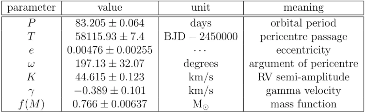
Then, they perform both multi-band photometry and radial velocity follow-up ob-servations to constrain the orbit and photometric variations further. For photometry follow-up observation, they use the Post Observatory Mayhill (POM). For radial ve-locity follow-up observation, they use the spectroscopy with the Tillinghast Reflector Echelle Spectrograph (TRES) on the 1.5 m Tillinghast Reflector at the Fred Lawrence Whipple Observatory (FLWO). They find that multi-band photometry show periodic variations inconsistent with stellar pulsations or ellipsoidal variations but consistent with spots from the shape of lightcurves. Besides, they find that in total 11 radial velocity data from TRES are well-fit by a near-sinusoidal curve. Table 2.3 shows the list of all measured radial velocities from TRES and Figure 2.2 shows the plot for them. Table 2.4 lists the best-fit orbital parameters they find from TRES.

Table 2.4 shows that the system has a near-circular orbit with the eccentricity

(15)

2.1 Examples of observed compact binary and triple systems 9 BJD-2450000 Relative RV(km/s) Uncertainty(km/s) 8006.9760 0.000 0.075 8023.9823 −43.313 0.075 8039.9004 −27.963 0.045 8051.9851 10.928 0.118 8070.9964 43.782 0.075 8099.8073 −30.033 0.054 8106.9178 −42.872 0.135 8112.8188 −44.863 0.088 8123.7971 −25.810 0.115 8136.6004 15.691 0.146 8143.7844 34.281 0.087

Table 2.3: Radial velocity measurements for 2M05215658+4359220 from data with TRES. In total, 11 spectra were obtained between 10 September 2017 and 25 January 2018. Adapted from Thompson et al. (2018).

parameter value unit meaning

P 83.205± 0.064 days orbital period

T 58115.93± 7.4 BJD− 2450000 pericentre passage

e 0.00476± 0.00255 · · · eccentricity

ω 197.13± 32.07 degrees argument of pericentre

K 44.615± 0.123 km/s RV semi-amplitude

γ −0.389 ± 0.101 km/s gamma velocity

f (M ) 0.766± 0.00637 M_⊙ mass function

Table 2.4: Best-fit orbital parameters from radial velocity follow-up observation with TRES. Adapted from Thompson et al. (2018).

f (M ) in Table 2.4 is computed from the observed variables K, Porb and e:

f (M )≡ K

3_P orb

2πG (1− e

2₎3₂_, _(2.5)

where K is the radial velocity semi-amplitude. Using equation (3.67), equation (2.5) reduces to f (M ) = M 3 COsin3iorb (Mgiant+ MCO) , (2.6)

where MCO is the mass of unseen companion, iorb is the orbital inclination, and Mgiant

is the mass of red giant 2M05215658+4359220. Therefore, the mass function is widely used to characterize the mass of unseen companion with the radial velocity observation. In order to analyze further, they assume that the system is tidally circularized and synchronized since Porb ≈ Pphot and e ≈ 0. Thus, for simplicity, they assume a fully

(16)

Figure 2.2: The radial velocity data for 2M05215658+4359220 from TRES follow-up observation. An error in each datum is within a filled circle.

parameter value meaning

MCO 3.2+1.1_−0.4 M⊙ mass of companion

Mgiant 3.0+0.6_−0.5 M⊙ mass of red giant

sin i 0.97+0.02_−0.14 orbital inclination

R 23.8+3.9_−0.6 R_⊙ radius of red giant

Table 2.5: Best-fit parameters from TRES, Gaia, and the SED. Adapted from Thomp-son et al. (2018).

synchronized and aligned orbit:

Prot = Porb = P, irot = iorb = i. (2.7)

Then, they search for the best-fit model in stellar evolution track with the surface gravity constraint log g = 2.35±0.14 from TRES spectroscopy, the giant radius R, the bolometric luminosity L and the eﬀective temperature Teﬀ from Gaia and the spectral

energy distribution (SED). This procedure reveals that best-fit value of companion mass lies on the range between the maximum neutron star and the minimum black hole masses from theoretical models. Table 2.5 summarizes the best-fit parameters.

Since log g for this sytem is known to include large systematic uncertainties (2.2≤ log g ≤ 2.6 depending on observation), they also try fitting procedure without the constraint on log g. Table 2.6 shows the result. However, they conclude that the best-fit values in Table 2.5 are better since the best-fit log g is found to be too small (log g≈ 1.7+0.2_−0.3) without constraint.

As a result, they reach a conclusion that 2M05215658+4359220 is a binary system consisting of a red giant and a possible black hole. However, there is the possibility

(17)

MCO 5.5+3.2_−2.2 M⊙ mass of companion

Mgiant 2.2+1.2_−0.9 M⊙ mass of red giant

sin i 0.65+0.17_−0.12 orbital inclination

R 35.8+8.3_−7.6 R_⊙ radius of red giant

Table 2.6: Same as Table 2.5 but derived without constraint on log g. Adapted from Thompson et al. (2018).

that the black hole is actually an unseen binary since it is not yet confirmed as a single object. Later, supposing that it is a binary rather than a single, we put a constraint on the binary as a practical application of our methodology.

2.1.3 A triple system PSR J0337+1715

As the final part of this section, we have a look at the discovery of a near-circular coplanar triple consisting of a white dwarf - millisecond pulsar binary and another outer white dwarf. If the motion of the outer white dwarf is precisely determined, this system would provide an ideal situation for our methodology. Thus, it is important since it implies the existence of the system for which the formulae derived in this thesis are directly applicable.

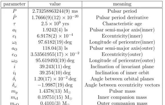
In 2014, Ransom et al. (2014) announced the discovery of a hierarchical triple consisting of a millisecond pulsar PSR J0337+1715, an inner white dwarf, and another outer white dwarf. As a part of large-scale pulsar survey, they discover a millisecond pulsar PSR J0337+1715 having a spin period of 2.73 ms with the Robert C. Byrd Green Bank Telescope (GBT). Since a millisecond pulsar emits the beams hundreds of times per second due to its rotation, the spin rate can be measured with high precision using pulse arriving time. In addition, analysing its delay in detail, it is possible to obtain the orbital information. At first, this system is considered to be a binary consisting of a millisecond pulsar and an inner white dwarf, however, the large timing systematics later reveal that the time delay is composed of two periodic variations with diﬀerent periods. This fact shows that this system should be classified into triple rather than binary. Although two other millisecond pulsars B1257+12 and B1620-26 have already known to have multiple companions, they contain planet-mass companions. On the other hand, large timing perturbations in PSR J0337+1715 implies more massive tertiary than a planet-mass companion.

In order to constrain the system’s position and orbital parameters, and the ter-tiary, they perform intensive multi-frequency radio timing campaign using the GBT, the Arecibo telescope, and the Westerbork Synthesis Radio Telescope (WSRT). The Arecibo has median arrival time uncertainties of 0.8 µs in 10 s. Thus, half-hour inte-grations achieve a precision of about 100 ns, which makes it possible to achieve one of the highest known precisions to PSR J0337+1715. They first approximate the motion as two Keplerian orbits, with the centre of inner binary moving around in the outer

(18)

P 2.73258863244(9) ms Pulsar period

˙

P 1.7666(9)(12)× 10−20 Pulsar period derivative

τ 2.5× 109 _yrs _{Characteristic age}

aI 1.9242(4) ls Pulsar semi-major axis(inner)

eI 6.9178(2)× 10−4 Eccentricity(inner)

ωI 97.6182(19) deg Longitude of pericentre(inner)

aO 118.04(3) ls Pulsar semi-major axis(outer)

eO 3.53561955(17)× 10−2 Eccentricity(outer)

ωO 95.619493(19) deg Longitude of pericentre(outer)

i 39.243(11) deg Inclination of invariant plane

iI 39.254(10) deg Inclination of inner orbit

δi 1.20(17)× 10−2deg Angle between orbital planes

δω −1.9987(19) deg Angle between eccentricity vectors

mp 1.4378(13) M⊙ Pulsar mass

mcI 0.19751(15) M⊙ Inner companion mass

mcO 0.4101(3) M⊙ Outer companion mass

Table 2.7: Best-fit system parameters for PSR J0337+1715. Note that values in parentheses are 1σ errors in the final decimal places. Adapted from Ransom et al. (2014).

orbit. Then, they determine pulse times of arrival (TOAs) using standard techniques and correct them to the Solar System barycentre at infinite frequency using a precise radio position obtained with the Very Long Baseline Array (VLBA). The variations of TOAs are known to have two physical origins. One is the “Rømer delay”, which is a geometric effect due to the finite speed of light. The other is the “Einstein delay”, which is a cumlative effect of time dilation due to the special relativistic transverse Doppler effect and the general relativistic gravitational redshift. The Rømer delay reflects the infomation on both inner and outer orbits.

Then, they plot the arrival timing data from the GBT, the WSRT, and the Arecibo telescope, and compare them with the Rømer delays model. They first calculate the residuals between data and two-Keplerian-orbit approximation. It shows the large systematic descrepancies up to several microseconds over multiple timescales, showing the presence of three-body interactions. Actually, these discrepancies contain much information about masses and geonetry of system. Thus, it is necessary to find param-eter sets minimizing the diﬀerence between measured TOAs and those by three-body integration. For this purpose, they use the Monte Carlo techniques to obtain the best-fit parameters. Table 2.7 summarizes the best-fit and derived parameters they find.

Besides, they suceed in identifying an object with blue colors in the Sloan Digital Sky Survey (SDSS). The optical spectroscopy reveals that it is consistent with a inner

(19)

2.2 Formation scenarios and observing proposals 13

white dwarf in the system confirmed by pulsar timing. It also shows that the outer companion cannot be a low-mass main-sequence star for lack of near- and mid- infrared excess, implying it should be a white dwarf with an eﬀective temperature less than 20000 K. Therefore, they finally conclude that the system is a triple consisting of a millisecond pulsar - white dwarf inner binary and another outer white dwarf.

This system is extremely surprising since its orbits are extraordinarily coplanar and near-circular. The authors propose a possible scenario to form such a system as follows. In a multiple star system, the most massive star experiences a supernove turning into a neutron star. Two companions survive the explosion, probably in eccentric orbits. After ∼ 109 _{yrs, the outermost star evolves and transfers mass onto inner}

binary. The angular momentum vectors of inner and outer orbits nearly align due to the torque during this process. After the outer star evolves into a white dwarf and another ∼ 109 _{yrs passes, the remaining main sequence star finally becomes a white}

dwarf. During this phase, the inner orbit becomes highly circularized and transfers small amount of mass to a neutron star, speeding up its rotation rate to form a millisecond pulsar. Then, three-body secular eﬀects have aligned the apsides of two orbits. Although this scenario is not yet fully confirmed whether or not to work well, it could produce near-circular and coplanar hierarchical triples if it can really take place.

2.2 Formation scenarios and observing proposals

Although the formation mechanism of compact binaries is not yet clearly understood, some scenarios have been proposed. These scenarios are roughly classified into three categories, isolated binary evolution, dynamical formation in star dense rigions, and primordial origin. Among these scenarios, the isolated binary evolution and dynamical formation scenarios are considered to be most promising ones. Since each scenario has characteristics for produced binaries, it is important to understand them. In this section, we briefly summarize two major scenarios (i.e. isolated binary evolution and dynamical formation) and their uniqueness especially on the preferred orbital parameters.

Besides, recently there are many observing proposals to search for star - black hole binaries with Gaia and TESS. Since Gaia and TESS have their own preferences for the property of detectable binaries, the knowledge on them is very useful to presume the binaries providing the targets to which we will apply our methodology. Thus, we also briefly summarize Yamaguchi et al. (2018) and Masuda & Hotokezaka (2018), which are proposals with Gaia and TESS, respectivaly.

2.2.1 Compact binary formation through isolated binary

evo-lution

The isolated binary evolution scenario (e.g. Belczy´nski & Bulik 1999; Belczynski et al. 2012, 2016, 2002, 2007; Dominik et al. 2012, 2013; Kinugawa et al. 2014, 2016) is

(20)

proposed as a most promising formation mechanism of close binary black holes. Apart from diﬀerences in detail concerns, overall picture of this scenario is summarized as follows.

This scenaio supposes presence of pre-existing binaries consisting of massive low-metal stars in the early universe. Since the typical lifetime of massive star is no more than ∼Myrs, the stars in a binary system quickly evolve oﬀ main sequence phases. First, one star in a binary evolves into a super redgiant and increase its radius drastically. Once the star fills in its Roche robe, significant mass flows into a companion, increasing the orbital separation and mass of companion. After the star finishes its super red giant phase, it evolves into a black hole via either direct collapse or non-violate supernova. During this phase, a star - black hole binary is formed. After a while, the companion also evolves into a giant phase. If the mass transfer is too strong to be stable, the unstable mass flow leads to the common-envelope phase, where the preformed black hole is absorbed by the envelope of the companion giant. During the common-envelope phase, since the orbital energy is consumed to eject the envelope, the orbital separation significantly decreases. Eventually, the giant also evolves into a black hole without a violate supernova. These successive processes preferentially form a close binary black hole. Since binary interactions such as the mass transfer and common-envelope phase well circularize an orbit, a typical produced binary tends to have vary small eccentricity e∼ 0.

Although it is confirmed that this scenario works well to produce close black hole binaries (e.g. Belczynski et al. 2016; Dominik et al. 2013; Kinugawa et al. 2014, 2016), there are many uncertainties in physical processes during this scenario. For example, it is known that violate common-envelope phase often leads to coalescense before compact binaries are formed although this process is important to form close binaries that merge within the age of universe. Since the eﬃciency of common-envelope phase is not yet clearly understood, this phase would change the surviving rate of close compact binaries. Even more serious problem raises up from uncertain supernova physics. Several previous researches (e.g. Belczy´nski & Bulik 1999; Belczynski et al. 2002; Kinugawa et al. 2014, 2016) found that significant mass loss and large natal kick due to supernova could produce wide and highly eccentric orbits although it simultaneously disrupts many binaries. If the direct collapse is really preferable for massive stars as proposed in Fryer et al. (2012), the natal kick and mass loss may be almost negligible. Thus, this scenario would produce massive compact binaries with circular close orbits.

No matter whether or not black hole binaries have initially eccentric orbits, the gravitational wave emission well circularizes the orbits after a long time evolution. Thus, the orbits are usually expected to have almost zero eccentricities before coales-cence. On the other hand, our methodology can detect wide and eccentric binaries if they exist since the methodology is irrelevant to coalescense. Our methodology could provide even new hints to understand currently uncertain supernova processes although careful checks are required to distinguish eccentric binaries formed via the dynamical formation scenario.

(21)

2.2.2 Compact binary formation through dynamical

interac-tions in star dense region

The dynamical formation scenario (e.g. O’Leary et al. 2009, 2006; Portegies Zwart & McMillan 2000; Rodriguez et al. 2016; Tagawa et al. 2016) is proposed as a counterpart of the isolated binary evolution scenario. While the isolated binary scenario requires pre-existing massive binary systems, the dynamical formation scenario enables single black holes to form binary black holes via strong gravitational interaction in star dense region. In this subsection, we have a look at the rough sketch of the dynamical formation scenario and the characteristics of the produced binaries.

Portegies Zwart & McMillan (2000) explored the possibility that black holes become close binaries via numerous gravitational scatterings with other members in star dense region, and estimate merger rate of the products. They found that this scenario could produce many black hole binaries even if their component black holes do not originally belong to binary systems. The overall picture of this scenario is summarized as follows. After all massive stars evolve oﬀ into black holes in star dense region such as globular cluster, black holes become most massive objects there. Since massive objects feel the dynamical friction strongly and lose kinetic energy, black holes tend to sink into the inner part of star dense region (e.g. Morris 1993). As a result of the condensation of black holes around core, many gravitational scattering and capture processes take place among black holes and other stars, resulting in the formation of binary black holes via three-body encounters. It is known that black holes preferencially form binary black holes with other black holes (e.g. Kulkarni et al. 1993). Therefore, the typical products may be binary black holes. While the close binary black holes become more tightly bound by superelastic encounter with other objects (e.g. Heggie 1975; Kulkarni et al. 1993), they are eventually ejected after getting the velocities large enough to escape from star dense region. Majority of these escaping binary black holes may have short enough orbital periods and high enough eccentricities that gravitational wave emissions lead them to coalescence within a few Gyrs.

In order to confirm this scenario, Portegies Zwart & McMillan (2000) performed N-body simulation with GRAPE-4, which is a special purpose computer for the multi-body problem. They used 2048 equal mass stars, with 1% of them 10 times more massive than the average (i.e. black holes). As a result, they found that ∼ 30% of in total 204 black holes were ejected from a cluster in the form of binary black holes,

∼ 61% were ejected in the form of single black holes, and ∼ 8% were retained by the

cluster. The binding energy of binary black holes Ebhad a roughly log-flat distribution

within the range of 1000kT − 10000kT , where (3/2)kT is mean stellar kiniteic energy in the cluster. The eccentricities of binaries roughly followed a thermal distirbution (p(e) ∼ 2e) with high eccentricities slightly overrepresented. They also found that ≳ 90% of black holes were ejected before the cluster had lost 30% of its initial mass (roughly within a few Gyrs).

After that, they estimated merger rate within 12 Gyr for typical star dense regions. The result is listed in Table 2.8. Table 2.8 shows that a variety of binary black holes may be formed depending on the properties of clusters although massive cluster tend

(22)

cluster type log M (M_⊙) log rvir (pc) 1000kT (R_⊙) Nbh fmerge (%) MR (Myr−1) populus 4.5 −0.4 420 7.9 7.7 0.0061 globular 5.5± 0.5 0.5 ± 0.3 315 150 51 0.0064 nucleus ∼ 7 ≲ 0 ≲ 3.3 2500 100 0.21 zero-age globular 6.0± 0.5 0± 0.3 33 500 92 0.038

Table 2.8: Typical parameters for each star dense region and expected merger rate. The M is the total mass and rvir is the virial radius. The fourth column denotes

the separation of binary consisting of two 10M_⊙ black holes to obtain 1000kT orbital energy. The Nbh is the expected number of binary black holes. The fmerge is the

fraction of these binaries which merge within 12Gyr. The final column denotes the contribution to the total black hole merger rate per cluster. Adapted from Portegies Zwart & McMillan (2000).

to produce tight binaries which merge soon after ejection.

O’Leary et al. (2006) systematically survey the distribution of eccentricities, orbital energies, and chirp masses for ejected binary black hole mergers. Instead of using ex-pensive N-body numerical simulation, they consider this scenario using a Monte Carlo technique to sample interaction rates, and few-body numerical simulation to treat each interaction. Thus, they succeeded to contain∼ 106 _{bodies including}_{∼ 500 black holes}

depending on models in their calculations. Since the ejected binary black holes are cir-cularized via gravitational wave emissions, their orbits are normally circular just before merger even though they tend to have high eccentricities when ejected. O’Leary et al. (2006) found that the eccentricities of almost all orbits would be less than 0.001 when their gravitational wave frequencies enter LIGO’s detectable range (∼ 10 Hz). They, however, found that LISA preferencially could detect the binary black holes with their eccentricities between 0.01 and 1 since LISA would have sensitivity around ∼ 10−3 Hz. More recent analysis including binary - binary interaction in general relativistic scheme (Zevin et al. 2018) also predicted that LISA would detect gravitational waves from binary black holes with eccentricities between∼ 0.00001 and ∼ 0.1 with the peak at∼ 0.001 around 10−2 Hz.

Therefore, apart from merger, the binary black holes formed dynamically will have high eccentricities. They found the chirp masses of merging binary black holes range from ∼ 10 to ∼ 100 although the distribution highly depend on models. They also computed the energy distribution of binary black holes ejected before equipartition using a model. They found that the energy distribution is nearly lognormal with a peak of ∼ 104_{kT between} _{∼ 100kT and ∼ 10}5_{kT , almost independent of models.}

The authors implied the discrepancy from Portegies Zwart & McMillan (2000) might be due to small number particles in the simulation in Portegies Zwart & McMillan (2000). Regardless, the results by Portegies Zwart & McMillan (2000) and O’Leary et al. (2006) may imply the presence of wider separation for ejected binary black holes.

(23)

Rodriguez et al. (2016) investigated the possibility that the progenitor binary black hole of GW150914 is formed by dynamical scenario. Although they did not calculate the distribution of orbital parameters since their concern was possible GW150914 progenitors, they found that the possible progenitors tend to have large eccentricities ≳ 0.5 and relatively wide separation ≳ 0.3 au at ejection. It probably imply the preference of eccentric and wider orbits indirectly. Interestingly, Rodriguez et al. (2016) found a temporary hierarchical triple consisting of blackholes among possible GW150914 progenitors during many scattering events although it was replaced by binary black holes before ejection. It may imply that this scenario could produce a hierarchical triple consisting of a star and inner binary black holes even though this class of objects are not much.

In summary, the dynamical scenario would provide relatively wider and highly eccentric binary black holes although it is not yet fully confirmed. Although grav-itational wave emission almost completely circularize the orbits before merger, our methodology can detect eccentric binaries from this scenario long before coalescence.

2.2.3 Observing proposals for binary systems including black

holes with Gaia

There are many proposals to search for star - black hole binaries using precise astrom-etry observation with Gaia(e.g. Breivik et al. 2017; Kawanaka et al. 2017; Mashian & Loeb 2017; Yamaguchi et al. 2018). Yamaguchi et al. (2018) suggest that Gaia can detect 200− 1000 binaries dependiong on the parameters in the isolated binary evolution model within 5 year operation. Since the binaries detected with Gaia will provide the targets to which we can apply our methodology, it is beneficial to know which kind of binaries Gaia will detect. In this subsection, we briefly summarize the proposal Yamaguchi et al. (2018) for this purpose.

First, Yamaguchi et al. (2018) estimate the number of star - black hole binaries in the Galaxy using the standard isolated binary formation scenario. They use the initial mass function of stars and binary distribution in terms of mass ratio of component stars, and estimate the number of binary systems. They assume that the initial sep-aration distribution of binaries is logarithmically flat, and binary orbits are circular initially. If the primary collapses into a black hole and the secondary still exists as a star, they count it as a star - black hole binary. In order to consider spatial distribution of such systems in the Galaxy, they use the exponentially decreasing number density in the Galactic plane. Since the systems in the Galactic bulge should not be detected due to strong interstellar absorption, they do not consider the systems located in the bulge. For simplicity, they assume that 50% of stellar systems are binaries. Taking into account the mass transfer and common-envelope phase during evolution, they can estimate the masses and separations of binary systems after evolution. They consider several diﬀerent values of paramaters describing the initial mass function, the binary distribution for a given mass ratio, the relation between zero-age mass and final black hole mass, and the common-envelope phase eﬃciency. They also take into account the

(24)

interstellar extinction to obtain detectable companions with Gaia.

Next, the authors consider the required condition to identify star - black hole binary systems with the standard errors in Gaia observation. For astrometry observation, we obtain (MBH+ M2)2 M3 BH = G 4π2 P_orb2 (a_∗D)3, (2.8)

where MBH and M2 are the masses of black hole and companion, respectively, Porb is

the orbital period, a_∗ is the angular semi-major axis, D is the distance. Thus, it is necessary to obtain Porb, a∗, D precisely to determine MBH. Through the discussion

on the standard errors of the observed quantities, the authors found the required condition for the semi-major axis of binary A:

A > 10MBH+ M2 MBH

σπ(mV)D ≡ Aast, (2.9)

where σπ(mV) is the Gaia standard error of parallax at a given apparent V -band

magnitude mV (Gaia Collaboration et al. 2016):

σπ(mV)≈

√

−1.631 + 680.8z(mV) + 32.73z2(mV), (2.10)

where

z(mV) = 100.4(max[12.09,mV]−15). (2.11)

Besides, they consider the required condition for semi-major axis from the viewpoint of orbital period. Considering the result from astrometry observation with Hipparcos, it is estimated that the standard errors in observed orbital periods are ≲ 10% if the periods are shorter than 2/3 of the total observation time. Since they consider 5 year oparation with Gaia in total, the upper limit of orbital period is∼ 3 years. In addition, since the observation cadence of Gaia is 50 days, the lower limit is 50 days. Therefore, the required condition for semi-major axis is

max[Aast, A(Porb = 50 days)] < A < A(Porb = 3 years). (2.12)

As a result, the authors found that in total 200− 1000 binaries would be detected with Gaia depending on the values of parameters. They also found that the detectable binaries would locate within 1− 10 kpc and the peak would be at 7 kpc. While the estimated number of binaries increases monotonically within ∼ 5 kpc due to larger volume, it drastically decreases after the peak ∼ 7 kpc. The distribution of black hole mass is sensitive to the parameters, especially the mass ratio of zero-age star and black hole. The distribution is the decreaing powerlaw within 4−30 M_⊙in the fiducial case. However, the maximum mass can reach∼ 100 M_⊙ if they assume high eﬃciency from zero-age star mass to black hole mass. They also found that the contribution of companion less massive that 20 M_⊙ is much smaller than those with larger masses. Since the mass ratio smaller than 0.3 undergo a strong common-envelope phase, the orbits might be too small to detect with Gaia.

(25)

In summary, considering the required condition (2.12), Gaia will provide the sys-tems which have relatively larger orbits with au-scale separations. It will be main diﬀerence between the systems TESS can detect. Although they do not consider the mass loss due to the stellar wind, natal kick, and initial eccentricity, they conclude that the countable black hole masses may not change drastically even including these eﬀects from the result in Breivik et al. (2017).

2.2.4 Observing proposals for binary systems including black

holes with TESS

Masuda & Hotokezaka (2018) recently point out that TESS will also detect star - black hole binaries via the photometric variations in light curves. While the typical targets of Gaia will be∼ 10 M_⊙ black holes in binary systems with their separations au-scale, Masuda & Hotokezaka (2018) find that the targets of TESS will be relatively tighter detached binaries with separations ≲ 0.3au. Thus, TESS will provide complementary samples of binary systems. In this subsection, we have a look at the observing proposal Masuda & Hotokezaka (2018).

First, they consider three kinds of effects in lightcurves that unseen massive com-panions induce. One is the “self-lensing”, which causes pulse-like periodic brightening due to microlensing during eclipse. Another is the “ellipsoidal variations”, which cause the phase-curve modulations induced by the change of geometrical shapse of stars due to tidal forces by massive companions. The other is the “Doppler beaming”, which is the special relativistic effect and causes the change of shape of light curves. Since they need consider the required conditions separately from self-lensing effect, they classify the latter two effects into the phase-curve variation. Although they concentrate on circular orbits throughaout their paper, this method will also be promising to detect the eccentric binaries.

Next, they computed the magnitude of each signal for given parameters to esti-mate the number of stars bright enough to detect the eﬀects above with TESS. They separately count the number of detectable stars for the self-lensing and phase-curve variation eﬀects. They define that the self-lensing is detectable if at least two pulses are observed. They define that the phase-curve variation is detectable if the binary period is less than half the observing duration. Since they are interested in detached stable binaries, they exclude the cases that the separation is within the Roche robe or strong gravitational wave emissions cause rapid orbital decays during observing du-ration. TESS performs photometric survey for transiting exoplanets around near-by stars. TESS will observe each sector for 27.4 days with 30 minute cadence usually. They use these values to estimate the number of targets.

They assume that the self-lensing signals are detectable if the following relation is satisfied: √ n ( ssl στ ) > 8.3, στ ≡ σ30 min ( _τ 30 min )_−0.5 , (2.13)

(26)

single pulse, and σ30 min is the noise level over 30 minute timescale corresponding to

one cadence. They used σ30 min by modifying σ1 houravailable in Stassun et al. (2018).

Equation (2.13) corresponds to the false-positive rate of ∼ 10−9 (Sullivan et al. 2015). For the phase-curve variation, they use the following required condition:

√ T 30 min ( s σ30 min ) > 10.4, (2.14)

where T is the observing duration, s is the amplitude of sine waves corresponding to phase-curve variation eﬀects. Equation (2.14) also corresponds to the false-positive rate of ∼ 10−9. Assuming that the inclination is random and using the TESS input catalog, which is a list of stars among which the target of TESS will be chosen, they found that ∼ O(107_{) and} _{∼ O(10}5_{) stars with periods up to} _{∼ 10 days would be}

bright enough to detect phase-curve variation and self-lensing, respectively. Since the self-lensing eﬀect is detectable only when the orbit is quite nearly edge-on, the number of targets is significantly smaller that that of phase-curve variation.

Next, they consider the occurrencre rate of star - black hole binaries based on two models. One is the “Field Binary model”, which is a simple estimation constructed by the combinatation of powerlaw occurence rate of black holes and that of massive binaries. The other is the “Common-envelope Evolution model”, which consider the common-envelope phase during evolution. Since they concentrate on large mass ratio, they need not consider the mass transfer as Yamaguchi et al. (2018). Combining the occurence rate and the result of searchable stars, they can construct the estimated number of detectable star - black hole binaries with TESS in terms of the mass of black hole and the orbital period.

As a result, regardless of the binary occurrence models, they found that TESS would detect ∼ O(10) and ∼ O(103) binaries by self-lensing and phase-curve vari-ation, respectively. Unlike the binaries which will be detected by Gaia, the tight binaries with 0.3− 30.0 day orbital periods will be detected by TESS. They found that the peak of orbital period was ∼ 5 days and the peak of mass was ∼ 20 M_⊙. Assuming 0.8 day orbital period and 7 M_⊙black hole, which is the representative value of X-ray black hole binaries, they estimated 0.25 kpc and 1.3 kpc as the maximum searchable distances for sun-like companions by self-lensing and phase-curve variation, respectively.

In summary, while Gaia is expected to detect wide-separation and massive binary systems beyond 1 kpc, TESS will detect the tight star - black hole binaries in near-by space. Since the performance of radial velocity method is the best for bright near-by stars, the binaries that TESS will find may provide good samples for our methodology.

(27)

Chapter 3 Perturbation theory to the

three-body problem

3.1 Two body problem

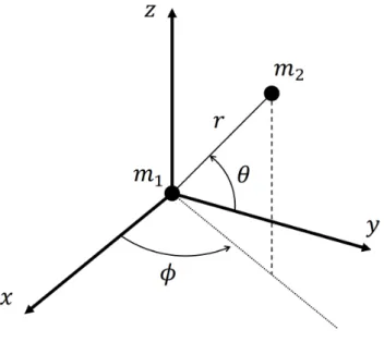
Before moving to the detailed formulation of three-body perturbation theory in celes-tial mechanics, we start from the simplest case for the motion under the gravitational interaction, i.e. the body problem. Many references are available for the two-body problem (Brouwer & Clemence 1961; Moulton 1914; Murray & Dermott 2000; Roy 2005, e.g.). This section specifically follows Murray & Dermott (2000). Con-sider two point particles with mass m1 and m2. They interact each other only by the

Newtonian gravitational force.

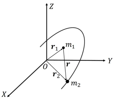
Figure 3.1 shows the configuration of the system that we consider here. In terms of an arbitrary Cartesian co-ordinate system (X, Y, Z), the equations of motion for the two particles are written as follows:

¨ r1 =−Gm2 (r1− r2) |r1− r2|3 (3.1) and ¨ r2 = Gm1 (r1− r2) |r1− r2|3 , (3.2)

where G is the universal gravitational constant, r1 and r2 are the position vectors of

m1 and m2, respectively. We introduce the position vector of the centre of mass R,

and the relative position vector r:

R≡ m1r1+ m2r2 m1+ m2 (3.3) and r ≡ r2− r1. (3.4) 21

(28)

22 Perturbation theory to the three-body problem

Figure 3.1: Two-body system in an arbitrary Cartesian co-ordinates

Using equations (3.3) and (3.4), we rewrite equations (3.1) and (3.2) to separate the motion of the centre of mass and the relative motion:

¨ R = 0 (3.5) and ¨ r =−Gmtotr r3 , (3.6)

where mtot is the total mass of the system. Equation (3.5) shows the centre of mass

moves with constant velocity.

Taking the vector product of r with equation (3.6), we obtain

r× ¨r = 0, (3.7)

thus,

r× ˙r = h, (3.8)

where h is a constant vector and called the “specific relative angular momentum”. Equation (3.8) shows that r and ˙r always lie on the invariant plane perpendicular to

h. This plane is called the “orbital plane”. Since we are interested in the relative

motion between two bodies, we concentrate on the motion fixed on the orbital plane using the result from equation (3.8).

(29)

3.1 Two body problem 23

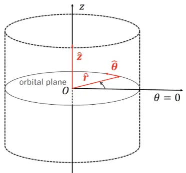
Figure 3.2: Cylindrical co-ordinate system.

Consider a cylindrical co-ordinate system (r, θ, z) with the origin at m1 as shown

in Figure 3.2. In the cylindrical co-ordinates, we can define basis vectors {ˆr, ˆθ, ˆz} as

ˆ r ≡   cos θsin θ 0   , ˆθ ≡   − sin θcos θ 0   , ˆz ≡   00 1   . (3.9)

Using these basis vectors, the position vector r, the velocity vector ˙r, and the

accel-eration vector ¨r are written as follows:

r = r ˆr, (3.10) ˙ r = d dt(r ˆr) = ˙r ˆr + r ˙ˆr = ˙r ˆr + r ˙θ ˆθ, (3.11) and ¨ r = d dt( ˙r) = ¨r ˆr + ˙r ˙ˆr + ˙r ˙θ ˆθ + r ¨θ ˆθ + r ˙θ˙ˆθ = (¨r− r ˙θ)ˆr + [ 1 r d dt(r 2_˙ θ) ] ˆ θ. (3.12)

Using equations (3.10) - (3.12), equations (3.6) and (3.8) become (¨r− r ˙θ2) ˆr =−Gmtot

(30)

and

h ˆz ≡ r2θ ˆ˙z = h. (3.14)

The areal element dA is

dA = 1 2|rˆr × rdθ ˆθ| = 1 2r 2 dθ. (3.15)

Thus, using equation (3.14), the areal velocity dA/dt is written as

dA dt = 1 2r 2_{θ =}_˙ 1 2h. (3.16)

Since h is constant, this equation shows that the areal velocity is also constant. This corresponds to Kepler’s second law.

In order to determine the orbit, we solve equation (3.13). Using u ≡ 1/r and equation (3.14), ˙r and ¨r are given by

˙r = −r2θ˙du dθ =−h du dθ (3.17) and ¨ r =−hu2r2θ˙d 2_u dθ2 =−h 2_u2d2u dθ2. (3.18)

Therefore, when we use u instead of r, equation (3.13) reduces to

d2_u

dθ2 + u =

Gmtot

h2 . (3.19)

Thie equations is solved as:

r = 1 u =

h2/Gmtot

1 + e cos(θ− ϖ), (3.20)

where e and ϖ are constants of integration and called the “eccentricity” and the “longitude of pericentre”, respectively. Equation (3.20) shows that when h ̸= 0, the orbit is ellipse (0 ≤ e < 1), parabola (e = 1) and hyperbola (e > 1) with m1 at the

focus (see Figure 3.3). Elliptical orbits correspond to Kepler’s first law.

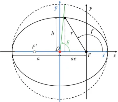
For an elliptical orbit, we can define semi-major axis a so that a(1−e) and a(1+e) become the minimum and maximum values of r, respectively. The point at which r takes the minimum value is called the “pericentre” and the point at which r takes the maximum is called the “apocentre”. If we introduce the “true anomaly” f as θ− ϖ, the pericentre and apocentre correspond to f = 0 and f = π, respectively (see Figure 3.4). The length b in Figure 3.4 is called the “semi-minor axis”. Using the fact that the summation of distances from two foci is equal for every point on an ellipse, we can express b in terms of a and e:

(31)

Figure 3.3: Classification of conical sections depending on eccentricity value.

Figure 3.4: Definition of the eccentric anomaly E. The dashed circle is the circum-scribed circle of ellipse with its centre at the centre of ellipse O. F and F′ denote the focus and the empty focus, respectively.

(32)

Using the semi-major axis and true anomaly, equation (3.20) is written as

r = a(1− e

2₎

1 + e cos f. (3.22)

This is a conventional expression for the elliptical Keplerian orbit.

Integrating equation (3.16) over one period of an elliptical orbit P , we obtain the following relation: 1 2hP = ∫ ellipse dA = πab = πa2√1− e2_. _(3.23)

Using equations (3.20) and (3.22),

h2 Gmtot

= a(1− e2) → h =√Gmtota(1− e2). (3.24)

Therefore, equation (3.23) becomes

P2 = 4π

2

Gmtot

a3. (3.25)

Equation (3.25) shows that the orbital period is independent of the eccentricity and only depends on semi-major axis and the total mass. This is Kepler’s third law.

Since the angle f covers 2π radians during one orbital period, we can introduce a kind of averaged angular velocity, the “mean motion”:

ν ≡ 2π

P , (3.26)

which characterizes the Keplerian motion. In terms of a and ν, equations (3.24) and (3.25) are written as

h = νa2√1− e2 _(3.27)

and

ν2a3 = Gmtot. (3.28)

We find that the specific angular momentum h is a constant of the motion. We next consider searching for another constant of the motion. Taking the scalar product

of ˙r with equation (3.6), ˙ r· ¨r = −Gmtot ˙ r· r r3 . (3.29) Thus, dC dt ≡ d dt ( 1 2r˙ 2₋Gmtot r ) = 0. (3.30)

Equation (3.30) shows that C is a constant of the motion. Since C denotes the orbital energy per unit mass, it is called the “vis viva integral” or “specific orbital energy”.

(33)

Consider writing C as a function of a, e, and mtot. Using equation (3.11), the square

of velocity ˙r2 _{can be written as}

˙

r2 = ˙r2+ (r ˙θ)2 = ˙r2+ (r ˙f )2, (3.31) where ˙θ = ˙f + ˙ϖ = ˙f . Using equations (3.16), (3.22) and (3.27),

r ˙f = h r = νa √ 1− e2(1 + e cos f ) (3.32) and ˙r = r ˙f e sin f 1 + e cos f = νa √ 1− e2e sin f. (3.33) Therefore, ˙r2 is written as ˙ r2 = ˙r2+ (r ˙f )2 = n 2_a2 1− e2(1 + 2e cos f + e 2₎ = ν 2_a2 1− e2 [ 2a(1− e2) r − (1 − e 2₎ ] = Gmtot ( 2 r − 1 a ) . (3.34)

The specific orbital energy C is written down using the equations above:

C = ( 1 2r˙ 2₋ Gmtot r ) =−Gmtot 2a . (3.35)

This equation shows that the orbital energy of elliptical motion is independent of the eccentricity and determined only by the semi-major axis and masses.

We have completed deriving the shape of orbit. However, the position of a body at a given time is still unknown. In order to determine the motion in a two-body problem, we derive the relation between the position and time as follows. Using equations (3.27), and (3.33) - (3.34), ˙r reduces to ˙r = √ ˙ r2− (r ˙f)2 ₌ νa r √ a2_e2− (r − a)2_. _(3.36)

In order to integrate equation (3.36), we can introduce the “eccentric anomaly” E instead of the true anomaly f (Figure 3.4).

The equation of a centred ellipse is (_x_¯ a )2 + (_y_¯ b )2 = 1, (3.37)

where a is the semi-major axis, b is the semi-minor axis, and (¯x, ¯y) is a set of

co-ordinates in rectangular co-co-ordinates with the origin at the centre of ellipse (see Figure 3.4). Considering equations (3.21) and (3.37), Figure 3.4 shows

¯

Radial velocity modulation of an outer star orbiting an unseen inner binary: analytic perturbation formulae in a three-body problem to search for wide-separation black-hole binaries

DISSERTATION