Playing Game 2048 with Deep Convolutional Neural Networks Trained by Supervised Learning

全文

(1)Vol.2018-GI-40 No.2 2018/6/29. IPSJ SIG Technical Report. Playing Game 2048 with Deep Convolutional Neural Networks Trained by Supervised Learning Naoki Kondo1,a). Kiminori Matsuzaki2,b). Abstract: Game 2048 is a stochastic single-player game and development of strong computer players for 2048 has. been based on N-tuple networks trained by reinforcement learning. Some computer players were developed with (convolutional) neural networks, but they did not perform well. In this study, we develop computer players for 2048 based on deep convolutional neural networks (DCNNs). We increment the number of convolutional layers from two to nine, while keeping the number of weights almost the same. We train the DCNNs by applying supervised learning with a large number of play records from existing strong computer players. The best average score achieved is 86,030 with five convolutional layers, and the best maximum score achieved is 401,912 with seven convolutional layers. These results are better than existing neural-network-based players, while our DCNNs have less weights. Keywords: game 2048, neural network, supervised learning. 1. Introduction Neural networks (NN) are now widely-used in the development of computer game players. Among them, deep convolutional neural networks (DCNN) have been studied actively in recent years and played an important role in the development of master-level computer players, for example, for Go (AlphaGo [13] and AlphaGo Zero [15]), Chess (Giraffe [6] and DeepChess [2]), Shogi (AlphaZero [14]), Poker (Poker-CNN [20] and DeepStack [10]), and Atari games [9]. The target of this study is game “2048” [1], a stochastic singleplayer game. Game 2048 is one of slide-and-merge games and its “easy to learn but hard to master” characteristics attracted quite a few people. According to its author, during the first three weeks after the release, people spent a total time of over 3000 years on playing the game. Several computer players have been developed for game 2048. Among them, the most successful approach is to use N-tuple networks (NTNs) as evaluation functions and apply a reinforcement learning method to adjust the weights of NTNs. This approach was first introduced to 2048 by Szubert and Ja´skowski [16], and then several studies were based on it. The state-of-the-art computer player developed by Ja´skowski [5] combined several techniques to improve NTN-based players, and achieved average score 609,104 under the time limit of 1 second per move. DCNN-based computer players, however, have not achieved a success yet. The only published work by Guei et al. [3] proposed a player with two convolutional layers followed by two 1. 2. a) b). Graduate School of Engineering, Kochi University of Technology Kami, Kochi 782–8502 JAPAN School of Information, Kochi University of Technology Kami, Kochi 782–8502 JAPAN [email protected] [email protected]. c 2018 Information Processing Society of Japan ⃝. full-connect layers but the average score was about 11,400. The player by tjwei [17] used two convolutional layers with a large number of weights with supervised learning and achieved average score 85,351. There exist some other implementations of DCNNbased players [12, 18], but the performance of these players were not reported. In this paper, we try to improve the performance of DCNNbased players by increasing the number of convolutional layers. We designed DCNNs with 2–9 convolutional layers and applied supervised learning with the play records of existing strong players [8]. As the result, we achieved better results than existing NN-based players. The best player with five convolutional layers achieved average score 86,030. The player with seven convolutional layers achieved maximum score 401,912. These results suggest that DCNNs with 5–7 convolutional layers have great potential to develop strong 2048 players. The rest of the paper is organized as follows. Section 2 briefly introduces the rule of game 2048. Section 3 reviews existing computer players for 2048, categorized in terms of N-tuple networks and neural networks. Section 4 shows the design of our DCNN players and explain how we applied supervised learning. Section 5 reports the experiment results. We discuss the findings in this study in Section 6, and conclude the paper in Section 7.. 2. Game 2048 The game 2048 is played on a 4 × 4 grid. The objective of the original 2048 game is to reach a 2048 tile by moving and merging the tiles on the board according to the rules below. In an initial state (Fig. 1), two tiles are put randomly with numbers 2 (p2 = 0.9) or 4 (p4 = 0.1). The player selects a direction (either up, right, down, or left), and then all the tiles will move in the selected direction. When two tiles of the same number collide they create a tile with the sum value and the player gets the. 1.

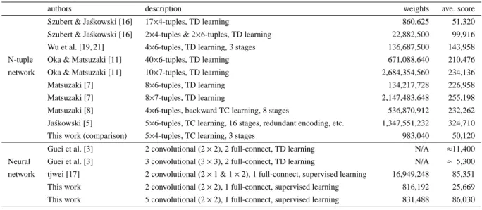
(2) Vol.2018-GI-40 No.2 2018/6/29. IPSJ SIG Technical Report. Table 1 Summary of players in terms of number of weights and average score of greedy play. (a). authors. description. weights. Szubert & Ja´skowski [16]. 17×4-tuples, TD learning. 860,625. 51,320. Szubert & Ja´skowski [16]. 2×4-tuples & 2×6-tuples, TD learning. 22,882,500. 99,916. Wu et al. [19, 21]. 4×6-tuples, TD learning, 3 stages. 136,687,500. 143,958. N-tuple. Oka & Matsuzaki [11]. 40×6-tuples, TD learning. 671,088,640. 210,476. network. Oka & Matsuzaki [11]. 10×7-tuples, TD learning. 2,684,354,560. 234,136. Matsuzaki [7]. 8×6-tuples, TD learning. 134,217,728. 226,958. Matsuzaki [7]. 8×7-tuples, TD learning. 2,147,483,648. 255,198. Matsuzaki [8]. 4×6-tuples, backward TC learning, 8 stages. 536,870,912. 232,262. 1,347,551,232. 324,710. Ja´skowski [5]. 5×6-tuples, TC learning, 16 stages, redundant encoding, etc.. This work (comparison). 5×4-tuples, TC learning, 3 stages. Guei et al. [3]. 2 convolutional (2 × 2), 2 full-connect, TD learning. Neural. Guei et al. [3]. 3 convolutional (3 × 3), 2 full-connect, TD learning. network. tjwei [17]. 2 convolutional (2 × 1 & 1 × 2), 1 full-connect, supervised learning. This work This work. 2. (b) 2. 2. 2. (c). 50,120. N/A. ≈11,400. N/A. ≈ 5,300 85,351. 2 convolutional (2 × 2), 1 full-connect, supervised learning. 816,192. 25,669. 5 convolutional (2 × 2), 1 full-connect, supervised learning. 831,488. 86,030. (c) 2. 4. 2. An example of the initial state. Two tiles are put randomly. After the first move: up. A new 2-tile appears at the lower-left corner. After the second move: right. Two 2-tiles are merged to a 4-tile, and score 4 is given. A new tile appears at the upper-left corner. Fig. 1 Process of game 2048. sum as the score. Here, the merges occur from the far side and newly created tiles do not merge again on the same move: move to the right from 222␣, ␣422 and 2222 results in ␣␣24, ␣␣44, and ␣␣44, respectively. Note that the player cannot select a direction in which no tiles move nor merge. After each move, a new tile appears randomly at an empty cell with number 2 (p2 = 0.9) or 4 (p4 = 0.1). If the player cannot move the tiles, the game ends. When we reach the first 1024-tile, the score is about 10,000. Similarly, the score is about 21,000 for a 2048-tile, about 46,000 for a 4096-tile, about 100,000 for an 8192-tile, about 220,000 for a 16384-tile, and about 480,000 for a 32768-tile.. 3. Existing 2048 players Table 1 summarizes the existing computer players in terms of their features, the number of weights, and the average score with greedy plays (i.e. without search methods). 3.1 Players based on N-Tuple Networks The most successful approach to computer 2048 players is based on N-tuple networks (NTNs) and reinforcement learning methods, which was first introduced by Szubert and Ja´skowski [16]. NTNs consist of a set of N-tuples and associated tables of (feature) weights. Given NTNs, we compute the evaluation value of a state simply by looking up weights corresponding to the tiles where the N-tuples cover. Thanks to the simple design and implementation of the NTNs, we can increase the number of also weights to improve the performance of players. We can also extend NTNs as follows.. c 2018 Information Processing Society of Japan ⃝. 983,040. 16,949,248. 2. (a) (b). ave. score. ( 1 ) Enlarge the size of tuples. Szubert and Ja´skowski [16] reported that the computer player performed significantly better by introducing 6-tuples instead of 4-tuples. Some studies used larger 7-tuples [5, 7, 11]. Note that a 4-tuple requires 164 = 65,536 weights, a 6-tuple does 166 = 16,777,216, and a 7-tuple does 167 = 268,435,456. ( 2 ) Increase the number of N-tuples. Though several studies have used four 6-tuples designed by Wu et al. [19], we can use more N-tuples if memory size permits. Oka and Matsuzaki [11] and Matsuzaki [7] analyzed the performance of players that utilizes many 6-tuples or 7-tuples. Ja´skowski’s redundant encoding is also a technique to increase the number of N-tuples (and we can save the number of weights with the use of smaller additional tuples). ( 3 ) Multi-staging. Multi-staging is a technique to divide a game into multiple stages and to use different tables of weights for each stage, which was first introduced by Wu et al. [19] for 2048. The feature weights are adjusted by reinforcement learning methods. For 2048 players, temporal difference learning (TD learning) was commonly used [16, 19, 21], and then a learningrate-free variant (temporal coherence learning) was introduced [5, 8]. Due to the characteristics of the game, biasing the boards to learn sometimes improves the performance, such as carousel shaping [5] and restart strategy [8]. The state-of-the-art player by Ja´skowski [5] was based on five 6-tuples networks adjusted by the temporal coherence learning with some other improvements, and achieved average score 324,710 with the greedy play and 609,104 with the expectimax search under the time limit of 1 second. Though NTNs have worked fine, a weakness remains: missing generalization. Since the weights are basically independent from each other, NTNs do not obtain some important property of the game (for example, the similarity among 1024–2048–4096 tiles and 2048–4096– 8192 tiles). Weight promotion [5, 8], which initializes a firstaccessed weight with a certain existing one, can be considered as a human-aided solution to this issue. A more affirmative reuse of feature weights achieved even a 65536-tile [4].. 2.

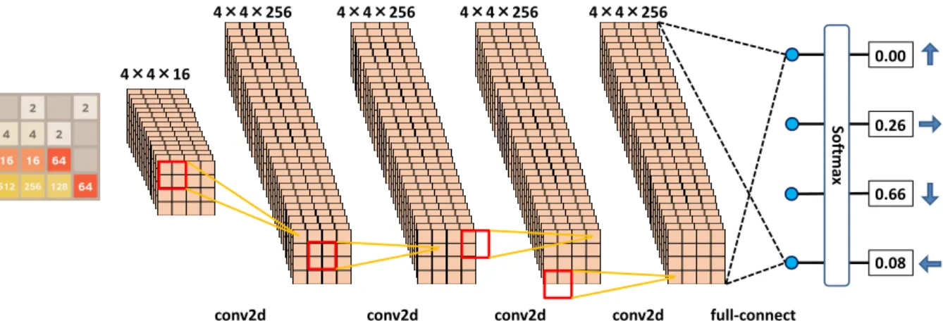
(3) Vol.2018-GI-40 No.2 2018/6/29. IPSJ SIG Technical Report. 4×4×256. 4×4×256. 4×4×256. 4×4×256 0.00. 4×4×16 Softmax. 0.26. 0.66. 0.08 conv2d. conv2d Fig. 2. 3.2 Players based on Neural Networks Behind the success of NTNs, (deep) neural networks have been less studied or utilized for the development of 2048 players. As far as the authors know, the work by Guei et al. [3] was the only published one. Some open-source programs have been developed, for instance, (convolutional) neural network player [17], deep Q-learning player [18], and deep recurrent neural network player [12], but the performance of these players was not analyzed well (at least from the documents provided). Guei et al. [3] first tried to develop 2048 players based on convolutional neural networks. They developed two networks, one with 2 × 2 filters and the other with 3 × 3 filters. The first network consists of two convolutional layers and two full-connect layers. The input board was encoded to a 4 × 4 16-channel image, where each channel corresponds to either empty-cells, 2-tiles, 4tiles, . . . , or 32768-tiles. Then, 2 × 2 filters are convoluted twice followed by ReLU, which result in 2 × 2 image (the number of filters for these convolutional layers was not described in the paper). The pixel values are flattened and then processed with two full-connect layers. The output consists of a single value (for TD learning) or four values (for Q learning). The second network is different from the first one in terms of the size of filters and the number of convolutional layers: 3 × 3 filters are convoluted (with zero padding) three times. The weights in these networks are adjusted by TD-learning and Q-learning methods with the results of selfplays. The best average score achieved with the first network was about 11,400 and with the second network about 5,300. The neural network developed by tjwei [17] consists of two convolutional layers followed by a full-connected layer. The input is a 4 × 4 16-channel image. In the first convolutional layer, 2 × 1 filters and 1 × 2 filters are applied concurrently and then ReLU, yielding a 3 × 4 512-channel image and a 4 × 3 512channel image. In the second convolutional layer, 2 × 1 filters and 1 × 2 filters are applied concurrently to both intermediate images, yielding four 4096-channel images. The pixel values are finally processed in a full-connected layer to a single output value. The average score achieved was 85,351 for the player trained with the supervised learning method.. c 2018 Information Processing Society of Japan ⃝. conv2d. conv2d. full-connect. Overview of our deep convolutional neural network. 4. Design In this study, we have designed deep convolutional neural networks (DCNNs) that have more convolutional layers than existing work [3, 17] and adjusted the weights by supervised learning with play records of existing strong players. In this section, we show the structure of designed DCNNs, the method of supervised learning, and the play method with the trained DCNNs. 4.1 Structure of Our DCNN As we reviewed in the previous section, existing NN-based players consisted of two (or three) convolutional layers. Since the game is played on a small 4 × 4 board, twice applications of convolution might cover the board. We, however, considered that those networks were too shallow to obtain good (and versatile) knowledge in the games, and designed DCNNs with more convolutional layers. Figure 2 depicts the structure of our DCNN for the case of four convolutional layers. In general, our DCNNs have k convolutional layers, a full-connected layer, and a softmax layer. The input board is encoded to a 4 × 4 16-channel image as the work by Guei et al. [3]. Each channel represents the positions of empty cells, 2-tiles, 4-tiles, . . . , and 32768-tiles, respectively. Then, 2 × 2 filters are convoluted k times. The stride width is one and zero padding is on so that the size of result images is also 4×4. We used the same number Ch(k) of filters (equals to the number of channels of intermediate images) for all the convolutional layers. Note that the convolution is asymmetric because the zero padding is applied only on the right and the bottom sides. After each convolution, ReLU is applied. After the convolutional layers, all the pixel values are processed in the full-connected layer that outputs four values. After the softmax layer, the four values represent probabilities of selecting the four directions. We selected the number Ch(k) so that designed DCNNs have almost the same number of weights to see the importance of depth of DCNNs. Table 2 shows the number of layers k, the number of channels Ch(k) and the number of weights in the DCNNs. Note that the numbers of weights are between 810,000–832,000, which are much smaller than that of existing players (only comparable to that of [16]).. 3.

(4) Vol.2018-GI-40 No.2 2018/6/29. IPSJ SIG Technical Report. Table 3 Example of state and its symmetries. Table 2 Numbers of convolutional layers, channels and weights Layers k. Channels Ch(k). Weights. 2. 436. 816,192. 3. 312. 818,688. 4. 256. 819,200. 5. 224. 831,488. 6. 200. 825,600. 7. 182. 818,272. 8. 168. 811,776. 9. 158. 819,072. 4.2 Supervised Learning Since the authors developed strong computer players for 2048 [8], we used play records of existing players as the training data of supervised learning. Since our DCNNs output probability P(i) for each move i, the supervised learning adjusts the weights to maximize the probability of the desired move. For this end, we defined the error E based on the cross entropy as follows. E=−. 3 ∑. t(i) log P(i). i=0.     1 where t(i) =    0. if i is the best move otherwise. We selected three players from the artifacts of our previous work [8] to generate the training data. These players utilized N-tuple networks as the evaluation functions: the networks consisted of four 6-tuples and the game was split to eight stages based on the maximum number of tiles. The weights of the networks were adjusted by backward temporal coherent learning with restart strategy. These players selected moves by the 3-ply expectimax search. The difference of the players was only in the weights. The average scores of the players were 459,455, 463,660 and 460,069. For the training data, we selected 6 × 108 boards from the play records of these players (these boards were from about 33,000 games). Each board was augmented with the move that the player selected, and we used the move to be the best move. Note that the training data were shuffled before fed to supervised learning. We would like to add short remarks about symmetry. The board and the rule of the game 2048 is rotation- and reflectionsymmetric, but the moves of a player are not usually symmetric. The N-tuple networks used in this study were trained in a completely symmetric manner, and the play records were not biased in terms of symmetry. Therefore, we did not feed symmetric boards in the training of DCNNs. 4.3 Playing Method As we discussed above, the training data were not biased in terms of symmetry, but the structure of DCNNs was asymmetric due to the implementation of zero padding. Therefore, in the playing, we generate eight symmetric boards and feed each of the eight boards to the DCNN. Table 3 gives an example. For each of the board, the DCNN returns the probabilities of the moves. We pick up the move with the largest probability and compute the corresponding move in the original board (written in the paren-. c 2018 Information Processing Society of Japan ⃝. up. 0.000. 0.000. 0.188. 0.095. right. 0.256. 0.178. 0.001. 0.644 (↓). down. 0.660 (↓). 0.560 (↓). 0.444 (→). 0.252. left. 0.084. 0.261. 0.367. 0.009. up. 0.673 (↓). 0.649 (↓). 0.317. 0.248. right. 0.083. 0.147. 0.372 (↓). 0.001. down. 0.000. 0.001. 0.312. 0.196. left. 0.244. 0.202. 0.000. 0.556 (↓). theses). We finally select the move to play with a majority vote. If two or more moves become the majority, we select the move based on the sum of probabilities. Since the training data were not biased, we had considered this use of symmetric boards worked insignificantly, but in fact it improved the score to a degree. Another design choice of selecting a move from symmetric ones was simply based on the sum of probabilities. This, however, performed worse than the majority vote.. 5. Experiments 5.1 Implementation and Experiment Settings We implemented the DCNN player using the TensorFlow framework. The supervised learning was executed with a batch of 1,000 boards. We used tf.train.AdamOptimizer for the optimization algorithm with the learning parameter 0.001. The initial values of weights were set randomly between −0.1 and 0.1. During the training phase, we observed the progress of learning through the error E and the accuracy. Here, the accuracy was calculated during the training using the training data themselves. After each training with 2 × 107 boards, the player took the snapshot of the weights and performed test plays of 1000 games. After the test plays, we calculate the average score, the maximum score, and the ratio of reaching 2048. 5.2 Experiment Results The progress of training was plotted in Fig. 3. We plotted the cases with two convolutional layers and five convolutional layers only, because the graphs for three to nine convolutional layers were quite similar. From Fig. 3, the training proceeded fast up to 1 × 108 boards, and did not stop even at 6 × 108 boards. We observed rather large oscillation of the error (and also the accuracy), and considered that this was caused by wide variety of states compared with the number of weights available. Table 4 summarized the error and the accuracy of selecting moves after training with 5.9–6.0 × 108 boards. Generally speaking, the smaller the error the larger the accuracy. The smallest error and highest accuracy were achieved with six convolutional layers, and the results of 3–8 convolutional layers would be within the oscillation. 4.

(5) Vol.2018-GI-40 No.2 2018/6/29. IPSJ SIG Technical Report. Table 5. Average score, maximum score, and ratio of reaching 2048. 1. average score. Average loss. 0.9. maximum. 2048. 2x conv2d. layers. 2 × 108. 4 × 108. 6 × 108. score. ratio. 5x conv2d. 2. 22,189. 25,530. 25,669. 175,628. 45.6. 3. 61,037. 64,212. 69,840. 332,868. 79.4. 4. 65,022. 73,054. 80,284. 343,496. 83.3. 5. 68,153. 73,435. 86,030. 385,560. 84.7. 6. 69,482. 74,441. 83,791. 387,376. 83.5. 7. 67,874. 77,448. 79,812. 401,912. 83.1. 8. 64,465. 74,737. 74,787. 363,916. 81.1. 9. 66,732. 73,484. 68,129. 358,736. 75.9. 0.8 0.7 0.6. 0.5 0.4 0. 1. 2 3 4 Training data (x 108). Fig. 3. 5. 6. Transition of error over learning. Table 4 The average error and accuracy during 5.9 × 108 – 6.0 × 108 actions. Average score (x 104). 39. 4. 46. 16384. 301. 307. 128. 188. 148. 1. 0. 412. 186. 36. 85. 8. 172. 387. 263. 11. 37. 66. 155. 394. 280. 18. 55. 33. 77. 152. 378. 284. 21. 2. 0.698. 0.692. 7. 27. 39. 103. 166. 382. 275. 8. 3. 0.543. 0.749. 8. 35. 51. 103. 190. 363. 245. 13. 4. 0.537. 0.750. 9. 50. 54. 137. 187. 348. 216. 8. 5. 0.535. 0.752. 6. 0.532. 0.755. 7. 0.544. 0.748. 8. 0.551. 0.751. 9. 0.552. 0.744. 2 0 1. 2. 3 4 Training data (x 108). 5. 6. Transition of average score over learning. max. 35 Best score (x104). 134. 39. 8192. 50. 4. ave. 109. 3. 4096. 6. 6. 40. 2. 2048. 5. 2x conv2d. 45. 1024. accuracy. 3x conv2d. Fig. 4. 512. error. 5x conv2d. 0. ≤256. layers. 10 8. Table 6 Distribution of maximum tiles layers. 30 25. We then plotted the average scores of test plays in Fig. 4. We selected the cases with 2, 3, and 5 convolutional layers: the graphs for 5 and 6 convolutional layers were close and the graphs for 4, 6, 7, 8 and 9 convolutional layers were between those of 3 and 5 convolutional layers at most of the points. Table 5 summarized the average scores of the test plays after the training of 2 × 108 , 4 × 108 and 6 × 108 boards, the maximum score over the whole test plays (up to training 6 × 108 boards), and the ratio of reaching 2048 after the training with 6 × 108 boards. The average scores and the maximum scores were also plotted in Fig. 5. From these figures and table, we claim that the player with two convolutional layers performed apparently worse than those with more convolutional layers. The best average score was 86,030 with five convolutional layers, which was a bit higher than the average score of tjwei’s player [17]. The best maximum score was 401,912 with seven convolutional layers. Note that the average score were still increasing at the training with 6 × 108 boards as we can see in Fig. 4. Table 6 summarized the number of test plays categorized by the maximum number of tiles at the game end. Unfortunately, the players could not reach a 32768-tile. The best player with six convolutional layers reached a 16384-tile in 2% of the games. This ratio was higher than that achieved by tjwei’s player [17], while the ratios of reaching 8192-, 4096- and 2048-tiles were lower.. 6. Discussion. 20 15 10 5. 0 2. Fig. 5. 3. 4 5 6 7 Number of conv2d layers. 8. Average score and maximum score of players. c 2018 Information Processing Society of Japan ⃝. 9. The most interesting result in this study is that the performance of the player improved significantly from two convolutional layers to three convolutional layers. Since the size of board is just 4 × 4, applying 2 × 2 filters twice would cover the whole board. One possible reason is related to generalization of knowledge obtained through the training phase. Let us consider combinations of tiles on an edge: [128, 64, 32, 16], [256, 128, 64, 32], and [512, 256, 128, 64]. There patterns often appear in good plays, 5.

(6) Vol.2018-GI-40 No.2 2018/6/29. IPSJ SIG Technical Report. and thus we would like to evaluate those patterns better. However, it would be impossible to obtain generalized knowledge with just two convolutional layers (we need to encode combinations independently in the weights). If we have three (or more) convolutional layers, we could encode the knowledge in the additional layer(s). This could be a reason why the players with three or more convolutional layers performed almost as the same level as the existing NN-based player [17], while the number of weights is much smaller. Of course, we could improve the performance by increasing the number of weights, but it is our future work to confirm it. It is also interesting that the results in this study are much better than those in the work by Guei et al. [3], even if the network consists of two convolutional layers. There could be several reasons for the improvement: the difference of learning method, that is, we used supervised learning instead of reinforcement learning; the number of weights available in the networks might be too small. Under the condition of a similar number of weights, the proposed DCNN players performed better than existing players including NTN-based ones . The first NTN-based player developed by Szubert and Ja´skowski achieved the average score 51,320. We also generated an NTN-based player with the techniques in [8], but the average score was almost the same. The best DCNN player achieved average score 86,030. One drawback of the proposed method is the long training time. In our preliminary tests, the training of DCNN players took 500 times longer than that of NTN players. Since we used only CPUs in the training, we could speed up the training by using GPUs.. Acknowledgment The training data used in this study were generated under the support of the IACP cluster in Kochi University of Technology. References [1] [2]. [3] [4] [5]. [6] [7]. [8]. [9] [10]. [11]. [12]. 7. Conclusion In this paper, we developed computer players for game 2048 based on deep convolutional neural networks trained by supervised learning. We changed the number of convolutional layers from two to nine while keeping the total number of weights. These networks were trained with the play records of existing strong computer players. The experiment results showed some interesting findings. The player with two convolutional layers did not perform well, and the players with three or more convolutional layers did much better, even with similar number of weights. The best player with five convolutional layers achieved the average score 86,030 without combining any search techniques, which was higher than existing NN-based players. The average score was also higher than that of NTN-based players under a similar number of weights. The player with seven convolutional layers achieved the maximum score 401,912, and this suggested that a deeper network would perform better if we could use more weights and training data. One of our future work is to identify the knowledge that our DCNN players have obtained by investigating the weights in the networks. We expect that the DCNNs successfully encoded some generalized knowledge, which is hard to obtain in N-tuple networks. We also want to increase the number of weights and training data and improve the performance of DCNN players for 2048.. c 2018 Information Processing Society of Japan ⃝. [13]. [14]. [15]. [16] [17] [18] [19]. [20] [21]. Cirulli, G.: 2048, http://gabrielecirulli.github.io/2048/ (2014). David, O. E., Netanyahu, N. S. and Wolf, L.: DeepChess: End-toEnd Deep Neural Network for Automatic Learning in Chess, International Conference on Artificial Neural Networks and Machine Learning (ICANN 2016), pp. 88–96 (2016). Guei, H., Wei, T., Huang, J.-B. and Wu, I.-C.: An Early Attempt at Applying Deep Reinforcement Learning to the Game 2048, Workshop on Neural Networks in Games (2016). Guei, H. and Wu, I.-C.: personal communication (2018). Ja´skowski, W.: Mastering 2048 with Delayed Temporal Coherence Learning, Multi-Stage Weight Promotion, Redundant Encoding and Carousel Shaping, IEEE Transactions on Computational Intelligence and AI in Games, Vol. 10, No. 1, pp. 3–14 (2018). Lai, M.: Giraffe: Using Deep Reinforcement Learning to Play Chess, Master’s thesis, Imperial College London, arXiv 1509.01549v1 (2015). Matsuzaki, K.: Systematic Selection of N-tuple Networks with Consideration of Interinfluence for Game 2048, Proceedings of the 2016 Conference on Technologies and Applications of Artificial Intelligence (TAAI 2016) (2016). Matsuzaki, K.: Developing 2048 Player with Backward Temporal Coherence Learning and Restart, Proceedings of Fifteenth International Conference on Advances in Computer Games (ACG2017), pp. 176– 187 (2017). Mnih, V., Kavukcuoglu, K., Silver, D., Graves, A., Antonoglou, I., Wierstra, D. and Riedmiller, M.: Playing Atari With Deep Reinforcement Learning, NIPS Deep Learning Workshop (2013). Moravc´ık, M., Schmid, M., Burch, N., Lisý, V., Morrill, D., Bard, N., Davis, T., Waugh, K., Johanson, M. and Bowling, M. H.: DeepStack: Expert-level artificial intelligence in heads-up no-limit poker, Science, Vol. 356, No. 6337, pp. 508–513 (2017). Oka, K. and Matsuzaki, K.: Systematic Selection of N-tuple Networks for 2048, Proceedings of 9th International Conference on Computers and Games (CG2016), Lecture Notes in Computer Science, Vol. 10068, Springer, pp. 81–92 (2016). Samir, M.: 2048 Deep Recurrent Reinforcement Learning. https: //github.com/georgwiese/2048-rl. Silver, D., Huang, A., Maddison, C. J., Guez, A., Sifre, L., van den Driessche, G., Schrittwieser, J., Antonoglou, I., Panneershelvam, V., Lanctot, M., Dieleman, S., Grewe, D., Nham, J., Kalchbrenner, N., Sutskever, I., Lillicrap, T., Leach, M., Kavukcuoglu, K., Graepel, T. and Hassabis, D.: Mastering the game of Go with deep neural networks and tree search, Nature, Vol. 529, No. 7587, pp. 484–489 (2016). Silver, D., Hubert, T., Schrittwieser, J., Antonoglou, I., Lai, M., Guez, A., Lanctot, M., Sifre, L., Kumaran, D., Graepel, T., Lillicrap, T., Simonyan, K. and Hassabis, D.: Mastering Chess and Shogi by Self-Play with a General Reinforcement Learning Algorithm, arXiv 1712.01815 (2017). Silver, D., Schrittwieser, J., Simonyan, K., Antonoglou, I., Huang, A., Guez, A., Hubert, T., Baker, L., Lai, M., Bolton, A., Chen, Y., Lillicrap, T., Hui, F., Sifre, L., van den Driessche, G., Graepel, T. and Hassabis, D.: Mastering the game of Go without human knowledge, Nature, Vol. 550, pp. 354–359 (2017). Szubert, M. and Ja´skowski, W.: Temporal Difference Learning of NTuple Networks for the Game 2048, 2014 IEEE Conference on Computational Intelligence and Games, pp. 1–8 (2014). tjwei: A Deep Learning AI for 2048. https://github.com/tjwei/ 2048-NN. Wiese, G.: 2048 Reinforcement Learning. https://github.com/ georgwiese/2048-rl. Wu, I.-C., Yeh, K.-H., Liang, C.-C., Chang, C.-C. and Chiang, H.: Multi-Stage Temporal Difference Learning for 2048, Technologies and Applications of Artificial Intelligence, Lecture Notes in Computer Science, Vol. 8916, pp. 366–378 (2014). Yakovenko, N., Cao, L., Raffel, C. and Fan, J.: Poker-CNN: A Pattern Learning Strategy for Making Draws and Bets in Poker Games, arXiv 1509.06731 (2015). Yeh, K.-H., Wu, I.-C., Hsueh, C.-H., Chang, C.-C., Liang, C.-C. and Chiang, H.: Multi-stage temporal difference learning for 2048-like games, IEEE Transactions on Computational Intelligence and AI in Games, Vol. 9, No. 4, pp. 369–380 (2016).. 6.

(7)