A Study on Gain Scheduling of Auxiliary Noise for Online Secondary and Feedback Path Modeling in Active Noise Control Systems

(1)

A Study on Gain Scheduling of

Auxiliary Noise for Online Secondary

and Feedback Path Modeling in Active

Noise Control Systems

by

Shakeel Ahmed

A thesis submitted in partial fulﬁlment

of the requirments for the degree of

Doctor of Engineering

Department of Communication Engineering and Informatics

Graduate School of Informatics and Engineering

The University of Electro-Communications

1-5-1 Chofugaoka, Chofu, 182-8585, Tokyo, Japan

(2)

Copyright

by

Shakeel Ahmed

(3)

DEDICATION

To my beloved parents, father Muhammad Javed; mother Sabia Beigum, and proﬁcient teachers for their invaluable support, and for guiding me to where I am

(4)

GLOSSARY

ADC Analog to digital converter. ANC Active noise control.

ANP Auxiliary-noise-power.

CEMFxLMS Computationally efficient modified filtered-x-least-mean-square. DAC Digital to analog converter.

DSP Digital signal processing. EMFN Even mirror Fourier non-linear. FBPM Feedback path modeling. FBPN Feedback path neutralization.

FBPMN Feedback path modeling and neutralization. FDAF Frequency domain adaptive ﬁlter.

FFT Fast Fourier transform. FIR Finite impulse response. FN Fourier non-linear.

FsLMS Filtered-s-least-mean-square. FxLMS Filtered-x-least-mean-square.

(5)

IIR Infinite impulse response. LMS Least-mean-square. MFxLMS Modified filtered-x-least-mean-square. MFxNLMS Modified filtered-x-normalized-least-mean-square. MNR Mean-noise-reduction. MSE Mean-square-error. NLMS Normalized-least-mean-square. NRP Noise-reduction-performance. OSPM Online secondary path modeling. PPSEQ Perfect-periodic-sequences. SNR Signal to noise ratio. SPM Secondary path modeling.

VFxLMS Volterra ﬁltered-x-least-mean-square. VSS Variable step-size.

(6)

SYMBOLS

d(n) Desired response/ Unwanted noise at the summing junction.

E[·] Mathematical expectation operator.

Eq Energy of signal q(n).

e(n) Residual error signal.

eq(n) Error signal of any adaptive ﬁlter Q(z).

f Signal frequency.

F (z) Feedback path transfer function with impulse response f (n). ˆ

F (z) Estimate of F (z) with impulse response ˆf (n). G(n) Time-varying gain.

G(n) Diagonal gain matrix.

G−1(n) Inverse of diagonal gain matrix.

k Frequency index.

Lq Length of any ﬁlter Q(z) and its estimate ˆQ(z).

n Time index.

P (z) Primary path transfer function with impulse response p(n).

(7)

Q(z) Filter transfer function with impulse response q(n).

Q−1(z) Inverse ﬁlter of Q(z) with impulse response q−1(n). ˆ

Q(z) Estimate of ﬁlter Q(z) with impulse response ˆq(n).

ˆ

Qo(z) Optimal value of the estimate ˆQ(z). ˆ

Q−1(z) Inverse ﬁlter of ˆQ(z) with impulse response ˆq−1(n).

q(n) Vector of length Lq containing tap-weights of ﬁlter Q(z)

Q(k) Complex conjugate of Q(k).

r(n) Noise from a noise source at reference microphone.

Rqq(n) Autocorrelation function of a signal q(n)

Rpq(n) Cross-correlation function of signal p(n) with q(n).

S(z) Secondary path transfer function with impulse response s(n). ˆ

S(z) Estimate of S(z) with impulse response ˆs(n). v(n) Auxiliary WGN used for system identiﬁcation.

vd(n) Measurement noise.

vg(n) Output of White noise generator.

vf(n) Output of F (z) corresponding to input v(n).

v_fˆ(n) Output of ˆF (z) corresponding to input v(n).

vs(n) Output of S(z) corresponding to input v(n).

vˆs(n) Output of ˆS(z) corresponding to input v(n).

x(n) Input excitation signal/ Noise signal from a noise source.

xq(n),x(n)(n) Input signal vector of ﬁlter Q(z) with input x(n) at iteration n

yq(n) Output signal of any adaptive ﬁlter Q(z).

ypq(n) Output of series combination of filters P (z) and Q(z) with input signal filtered first through P (z) and then through Q(z).

(8)

∆ Delay.

∆Dq(n) Relative modeling error of ﬁlter Q(z).

δ(n) Unit sample function.

∆X Mean-square-error in the signal r(n).

|| · ||2 _{Square of the Euclidean norm.}

λ Forgetting factor.

µ Fixed step-size parameter for an adaptive ﬁlter.

µq(n) Time-varying step-size parameter for adaptive ﬁlter Q(z).

µq(n) Diagonal matrix of time-varying step-size parameters for adaptive ﬁlter Q(z).

(9)

概　　要

アンチノイズ信号を生成して音響ノイズをキャンセルする非常に興味深い手法は，1936 年に P. Lueg によって提案された．フィードフォワード型アクティブノイズコントロール (ANC) システムでは，アンチノイズ信号は，基準マイクとエラーマイク，ANC フィルタに基づく適応 FxLMS (Filtered-x-Least-Mean-Square) アルゴリズム及び電気音響二次経路により生成される．ANC システムが安定に動作するには，FxLMS アルゴリズムが二次経路の推定が必要である．スピーカーで生成されたアンチノイズ信号が基準マイク信号と干渉を引き起こす．この干渉はスピーカーと基準マイクの間にフィードバック経路と呼ばれる電気音響経路が存在することに起因する．よって，このフィードバック経路の影響を中和する必要があり，フィードバック経路の推定が必要である．二次経路とフィードバック経路のオンラインモデリングのために，付加的な補助ノイズが注入される．この補助ノイズは，残留誤差を招き，ANC システムのノイズ低減性能 (NRP) を劣化させる．NRP を改善するために，ゲインスケジューリング手法が使われ，注入された補助ノイズの電力を変化させる．ゲインスケジューリングの目的は，二次経路とフィードバック経路のモデル推定値が実際の未知経路とかけ離れているとき，大きい補助ノイズを注入して高速に収束させることである．推定値が実際の未知経路に近いときは，補助ノイズを小さい値に低減させる．したがって，ゲインスケジューリングは，二次経路とフィードバック経路のモデル推定に役に立つと同時に，定常状態では NRP を改善できる．本論文では，二つの重要な問題：オンライン二次経路モデリング (OSPM) と、オンラインフィードバック経路モデリングとニュートラリゼション (FBPMN) について，ゲインスケジューリングの幾つか異なる方法を提案する．第１章では，まず ANC システムの基礎となる物理的原理と構成について概説する．異なるシステム同定において，ANC システム，すなわち，適応フィルタの基本構成ブロックの適用について議論し，ANC システムの中で最もよく使われている適応アルゴリズム，すなわち，FxLMS アルゴリズムを一般的な二次経路のために導出する．また，ANC システムにおける二つの基本的な問題：OSPM とオンライン FBPMN について説明し，システム同定のための最適な励起信号，すなわち，完全スイープ信号の使用についても述べる．第２章では，分散値を固定した補助ノイズを使用した条件でゲインスケジューリングなしの OSPM について，既存の手法を解説し，修正された FxLMS (MFxLMS) と OSPM のための簡単な構造を持つ適応アルゴリズムを提案する．提案した簡単な構造の利点は，ANC システムの性能を維持しなが

(10)

ら，MFxLMS アルゴリズムに基づく OSPM の計算量を低減できることである．また，シミュレーションを行い，その結果を用いて既存の方法と性能を比較する．第３章では，まず，ゲインスケジューリングを用いた OSPM について，既存の手法を解説する．既存のゲインスケジューリング手法の利点と欠点を分析し，新しいゲインスケジューリング手法を提案し，SPM フィルタのモデリング精度および ANC システムの NRP を改善する．既存の方法では，ANC システムの収束状態の情報のみを持つ残差信号の電力に基づいてゲインを変動させる．一方，提案法では，SPM フィルタのエラー信号の電力に基づいてゲインを変動させている．SPM フィルタのエラー信号の電力は ANC システムと SPM フィルタの両方の収束状態に関する情報を持つため，ゲインを制御するより望ましい手法である．また，シミュレーションを行い，その結果を用いて既存の方法と性能を比較する．第４章では，ANC システムのフィードフォワード構成に関連するオンライン FBPMN の問題について議論する．はじめに，ゲインスケジューリングを使用しないオンライン FBPMN について，既存の方法とそれらの問題点を説明する．つぎに，ゲインスケジューリングを使用しないオンライン FBPMN のための新しい構造を提案し，シミュレーションを行い，既存の方法と性能を比較する．新しい構造では，既存構造の特長が組み合わせられ，予測器を使って適応 FBPMN フィルタのエラー信号から予測可能な干渉項を除去する．加えて， FBPM フィルタと FBPN フィルタが単一の FBPMN フィルタとして結合される．既存構造に比較して，新しい構造の利点は，ANC フィルタの入力信号にフィードバックカップリングする作用をより良く中和でき，ANC システムの収束性を改善することができる．後半では，ANC システムの NRP を改善するために，ゲインスケジューリング手法を提案する．また，FBPMN フィルタのステップサイズが一致する自己同調 ANP スケジューリング手法も提案する．この自己同調 ANP スケジューリング手法では，チューニングパラメータを必要とせず，ANC システムの NRP をさらに改善できる．第５章では，本論文の結論と今後の研究課題等について述べる．

(11)

ABSTRACT

The idea of cancelling the acoustic noise by generating an anti-noise signal is very fascinating, and was first proposed by P. Lueg in 1936. In feedforward active noise control (ANC) systems, the anti-noise signal is generated with the help of reference and error microphones, an adaptive filtered-x-LMS (FxLMS) algorithm based ANC filter, and an electro-acoustic path named as the secondary path. For stable operation of ANC systems, the FxLMS algorithm needs an estimate of the secondary path. The anti-noise signal generated by the loudspeaker (part of secondary path) causes interference with the reference microphone signal. This interference is due to the presence of electro-acoustic path, named as feedback path, between the loudspeaker and the reference microphone. It is required to neutralize the effect of this feedback path, and hence an estimate of the feedback path is required.

For online modeling of the secondary and feedback paths, an additional aux-iliary noise is injected. This auxaux-iliary noise contributes to the residual error, and thus degrades the noise-reduction-performance (NRP) of ANC system. In order to improve the NRP, a gain scheduling strategy is used to vary the variance of the injected auxiliary noise. The purpose of the gain scheduling is that when the model estimates of the secondary and the feedback paths are far from the actual unknown paths, auxiliary noise with large variance is injected. Once the model estimates are closer to the actual unknown paths, the variance of auxiliary noise is reduced to a small value. In this way, on one hand the gain scheduling can help us to achieve the required model estimates of secondary and feedback paths, and on the other hand to improve the NRP at the steady-state. In this thesis, we discuss the two most important issues, i.e., 1) online secondary path modeling (OSPM), and 2) online feedback path modeling and neutralization (FBPMN) with gain scheduling.

In chapter 1, the basic underlying physical principle and configurations of active noise control (ANC) systems are explained. The application of the basic building block of an ANC system i.e. An adaptive filter, in different system iden-tification scenarios is discussed. The most popular adaptive algorithm for ANC system, i.e., FxLMS algorithm is derived for the general secondary path. A brief overview is given for the two fundamental issues in ANC systems, i.e., 1) OSPM

(12)

and 2) online FBPMN. The use of optimal excitation signal, i.e., Perfect sweep

signals for system identiﬁcation is described.

In chapter 2, the existing methods for OSPM without gain scheduling, where the auxiliary noise with fixed variance is used in all operating conditions, are dis-cussed. In this chapter a simplified structure for OSPM with the modified FxLMS (MFxLMS) adaptive algorithm is proposed. The advantage of the simplified struc-ture is that it reduces the computational complexity of the MFxLMS algorithm based OSPM without having any compromise on the performance of ANC system. In chapter 3, the existing methods for OSPM with gain scheduling are dis-cussed. The drawbacks with the existing gain scheduling strategies are highlighted, and some new gain scheduling strategies are proposed to improve the modeling ac-curacy of SPM filter and the NRP of an ANC system. In existing methods, the gain is varied based on the power of residual error signal which carries information only about the convergence status of ANC system. In the Proposed methods the gain is varied based on the power of error signal of SPM filter. This is more de-sirable way of controlling the gain because the power of error signal of SPM filter carries information about the convergence status of both the ANC system and the SPM filter. The performance comparison is carried out through the simulation results.

In chapter 4, the second most important issue associated with the feedforward configuration of ANC system, i.e., the issue of online FBPMN is deal with. In the first part, the existing methods for online FBPMN without gain scheduling are dis-cussed. A new structure is proposed for online FBPMN without gain scheduling. The performance of the existing methods is compare with the proposed method through the simulation results. In the new structure the good features from the existing structures are combined together. The predictor is used in the new struc-ture to remove the predictable interference term from the error signal of adaptive FBPMN filter. In addition to this, the action of FBPM filter and the FBPN fil-ter is combined into a single FBPMN filfil-ter. The advantage of the new structure over the existing structures is that it can better neutralize the effect of feedback coupling on the input signal of ANC filter, thus improves the convergence of ANC system. In the second part, a gain scheduling strategy is proposed to improve the NRP of ANC system. In addition to this, a self-tuned ANP scheduling strategy with matching step-size for FBPMN filter is also proposed that requires no tuning parameters and further improves the NRP of ANC systems.

In chapter 5, the concluding remarks and some future research directions are given.

(13)

Chapter 1 Introduction

1.1 Active Noise Control (ANC)

Noise is an unwanted or an undesired signal. The unintended and undesired sound in the acoustic domain is called acoustic noise. The major sources of the acoustic noise include industries, and transportation. Broadly speaking the acoustic noise can be classiﬁed into two major types; 1) Narrow band noise, having energy con-centrated at speciﬁc frequencies, e.g., noise from rotating machines and engines etc., and 2) Broad-band noise, having energy distribution over a broad range of audible frequencies, e.g., pink noise, white noise etc [1]-[5].

The traditional approach for acoustic noise cancellation is to use the passive techniques. These techniques include the use of sound absorbing materials,

(17)

si-Noise

Anti-Noise Residual Noise

Figure 1.1: Physical concept of active noise cancellation.

lencers, enclosures, barriers, and mufflers [1, 2] for noise attenuation. These pas-sive techniques are effective at high frequencies, and become ineffective, large in size, and costly at low frequencies (for f < 500Hz). The alternate solution at low frequency is to use active techniques for noise cancellation [3]- [5].

Physical concept of ANC: The basic building block of an ANC system is an adaptive filter [6]-[8], and the underlying physical concept is the principle of superposition. In feedforward configuration of ANC systems, using the reference microphone signal, the electrical adaptive controller followed by the secondary path will generate an anti-noise signal. The anti-noise signal will interfere destruc-tively with the unwanted noise signal at the summing junction, and will cancel the original noise. The better cancellation will be achieved if the magnitude of the anti-noise is same and phase is exactly opposite to that of original unwanted noise. The idea of noise cancellation with an anti-noise signal is shown in Fig. 1.1. It is difficult to achieve the desired performance with analog circuits, hence it is required for the controller of ANC system to be digital [4].

The idea of using the microphones and the secondary source (loudspeaker) to generate the anti-noise signal was ﬁrst proposed by P. Lueg in 1936 [9]. Since the characteristics of the unwanted noise, and the acoustic paths are time-varying, therefore the idea presented in [9] did not have the practical applications until the

(18)

development of adaptive signal processing algorithm and DSP hardware. The idea became practically realizable with the development of adaptive signal processing algorithm and DSP hardware in 1980. The application of adaptive signal process-ing to cancel the noise in a duct was proposed in [10]-[12], where the adaptive ﬁlters adjust its coeﬃcients to minimize some cost functions.

Basic configurations of ANC systems: Based on the structure, the ANC systems can be classified into following two types: 1) Feedforward Single/Multi channel ANC system, and 2) Feedback Single/Multi channel ANC system. The feedforward ANC system can be used to cancel both the narrow-band (predictable) as well as the broad-band (unpredictable) noise signals, whereas the feedback ANC system is used to cancel only the narrow-band signal. The feedback ANC system can not be employed for the cancellation of broad-band noise signal due to inherent delay associated with the feedback configuration. The details for the feedforward and feedback ANC system can be found in [3]- [5].

ANC applications: When the unwanted noise to be canceled is at high fre-quency, the need of high sampling rate will limit the use of active techniques, so passive techniques are the best choice. However on the other hand, when the unwanted noise is at low frequency, active techniques are the obvious choice due to size and cost constraints. ANC has found many applications such as in cars, locomotives, air-planes, particularly hi-tech propeller driven air crafts, helicopters, ships, and boats to cancel the unwanted noise coming from an engine. ANC can be employed in smart-phones, earphones, and blue-tooth head sets to cancel the background noise and allow the user to hear a clean audio of a song, or news etc. The most popular applications of ANC systems are in ventilations, air condition-ing ducts used in seminar rooms, hospitals, concert halls and meetcondition-ing rooms [4].

(19)

In this thesis, our focus will be on the application of ANC in acoustic duct.

1.2 Adaptive Filtering in ANC

The adaptive filter is one of the basic building block of an adaptive ANC system. An adaptive filter can be realized using FIR or IIR structure. In this thesis, the FIR structure will be used for the implementation of an adaptive filter. In an adaptive filter, the coefficients are adjusted automatically such that a certain cost function is minimized. The adaptive filtering finds many applications in area of an unknown system identification [7], prediction [13], and inverse filtering.

System identification: The block diagram for an unknown system identifi-cation using an adaptive filter is shown in Fig. 1.2, where W (z) is the transfer function of an unknown system, ˆW (z) is an adaptive filter and represents an

esti-mate of W (z), yw(n) and ywˆ(n) are the outputs of W (z) and ˆW (z), respectively,

corresponding to input excitation signal x(n), vd(n) is a measurement noise and usually modeled as additive white Gaussian noise (WGN), d(n) is the desired re-sponse of adaptive ﬁlter, and ewˆ(n) is the error signal of adaptive ﬁlter ˆW (z).

The adaptive filter updates its coefficient at each iteration such that the certain cost function is minimized. Acoustic echo cancellation [14] is one of the practical application where system identification is required.

Prediction: The general block diagram of an adaptive linear predictor is shown in Fig. 1.3. It is called predictor because the current value of the in-put x(n) is predicted from the past sample values of x(n). If it is assumed that the adaptive ﬁlter has length Lw, then the output ywˆ(n) can be written as the linear

(20)

Figure 1.2: Adaptive system identiﬁcation.

Figure 1.3: Adaptive linear prediction.

combination of the past sample values of x(n), and is computed as

ywˆ(n) = ˆw(n)∗ x(n − ∆) = ˆwT(n)xw(n),x(nˆ −∆)(n), (1.1)

where ˆw(n) is the impulse response of ˆW (z), x(n−∆) is the delayed version of x(n),

ˆ

w(n) = [ ˆw0(n), ˆw1(n),· · · , ˆwLw−1(n)]

T _{is the impulse response coeﬃcient vector of} adaptive ﬁlter ˆW (z) at time n, xw(n),x(nˆ −∆)(n) = [x(n−∆), x(n−∆−1), · · · , x(n−

∆−Lw+ 1)]T is the input signal vector of ˆW (z) with input x(n−∆) at time n, and ∆ represents the delay. This technique is useful in some applications where it is required to separate the predictable signal from the unwanted random background noise.

(21)

(a)

(b)

Figure 1.4: Adaptive inverse ﬁltering: (a) Unknown system followed by an adaptive

ﬁlter, (b) Adaptive ﬁlter followed by an unknown system.

Inverse filtering: The general block diagram for inverse filtering in two sce-narios is shown in Fig. 1.4. In inverse filtering, the coefficients of the adaptive filter ˆW (z) are updated in such a way that the overall impulse response is the unit

sample function, i.e, ˆw(n)∗ ˆw−1(n) = δ(n), where ˆw(n) is the impulse response of

ˆ

W (z), ˆw−1(n) is the impulse response of ˆW−1(z), and δ(n) is the unit sample func-tion. The block diagram in Fig. 1.4(a) is used in communication systems, where it is required to equalize the eﬀect of the channel on the transmitted signal. The block diagram in Fig. 1.4(b) has found application in ANC, where the controller is required to equalize the eﬀect of the secondary path [4].

(22)

Noise Source Loudspeaker _Error Microphone Reference Microphone Duct

Figure 1.5: LMS adaptive algorithm based ANC for acoustic duct: An example of

indirect system identiﬁcation.

Direct VS Indirect system identification: In direct system identification the output of an adaptive filter is subtracted from the desired response d(n), as shown in Fig. 1.2 _{∼ Fig. 1.4(a), whereas in indirect system identification, the} output of an adaptive filter has to pass through some filters before being subtracted from the desired response, as shown in Fig. 1.4(b). The practical example of an indirect system identification is an ANC system, where the electrical adaptive controller is followed by an electro-acoustic secondary path.

ANC for acoustic duct (an example of indirect system identiﬁcation): The block diagram of a single channel feedforward LMS adaptive algorithm based ANC system for acoustic duct is shown in Fig. 1.5. Here x(n) is the unwanted noise to be canceled. This unwanted noise travels through an electro-acoustic path P (z). The transfer function P (z) represents the combination of the transfer functions

P′(z) and R(z), i. e., P (z) = P′(z)R(z). The transfer function P′(z) includes the transfer function of the acoustic path from the reference microphone to the summing junction, and R(z) is the residual transfer function from the summing junction to the residual error signal e(n). The transfer function R(z) includes not only the transfer function of the acoustic path from the summing junction to the error microphone, but also the transfer functions of error microphone,

(23)

pre-ampliﬁer, anti-aliasing ﬁlter, and analog to digital converter (ADC). The signal

x(n) is also picked-up by the reference microphone and is given to the controller W (z). The output yw(n) of W (z) is applied to secondary path transfer function

S(z) to generate yws(n) (estimate of d(n)). Similar to P (z), the secondary path transfer function S(z) also represents the combination of the transfer functions

S′(z) and R(z). The transfer function S′(z) includes the transfer function from the controller output yw(n) to the summing junction [4]. The transfer functions

P (z) and W (z)S(z) will transform the signal x(n) to d(n) and yws(n), respectively. The signal d(n) and its estimate yws(n) will interfere with each other destructively (note the negative sign at the error microphone in Fig. 1.5 to reduce the noise at the summing junction.

In Fig. 1.5, the controller W (z) will simultaneously identify P (z) (indirect system identiﬁcation) and equalize S(z), i.e., W (z) = ˆP (z) ˆS−1(z), where ˆP (z)

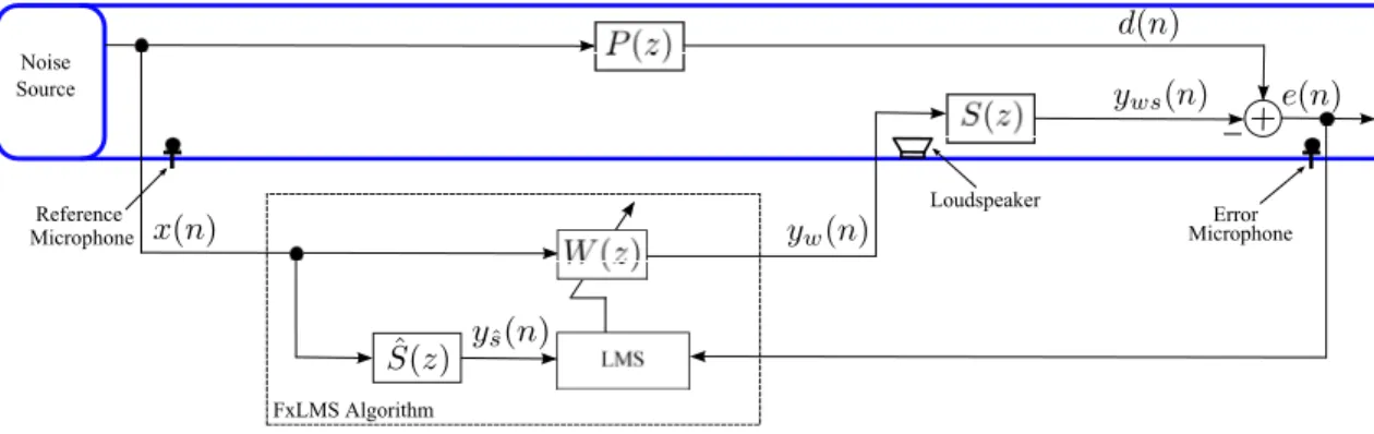
and ˆS−1(z) are the estimate of P (z), and inverse transfer function of S(z). If it is assumed that the secondary path is linear, then the filters W (z), and S(z) can commute. With this commutation the problem of indirect system identification is now transformed to direct system identification and is shown in Fig. 1.6. It is clear from Fig. 1.6 that the input signal x(n) is filtered through the secondary path before being applied to the adaptive algorithm of W (z). Therefore, the assumption of the linearity of the secondary path led to the foundation of the most popular filtered-x-LMS (FxLMS) algorithm [15]. The FxLMS algorithm was also derived independently by Burgess and Widrow in [10], and [16], respectively. The equivalent block diagram of FxLMS algorithm based single channel feedforward ANC system for duct is shown in Fig. 1.7, where ˆS(z) represents the estimate of S(z).

(24)

Noise Source

Figure 1.6: Block diagram of ANC system with secondary path followed by

con-troller. Reference Microphone Loudspeaker Error Microphone Noise Source FxLMS Algorithm

Figure 1.7: FxLMS algorithm based single channel feedforward ANC system for

duct.

1.2.1 FxLMS Algorithm for General Secondary Path

In the case of ANC systems the secondary path can be linear or nonlinear. In this section, at ﬁrst the expression of FxLMS algorithm is derived for general secondary path. After that, the assumption of the linearity of the secondary path is incorporated into the general expression to have an expression for the FxLMS with linear secondary path. From Fig. 1.7, the residual error signal e(n) is given by

(25)

where

d(n) = p(n)∗ x(n) = pT(n)xp(n),x(n)(n), (1.3) and

yws(n) = s(n)∗ yw(n) = sT(n)xs(n),yw(n)(n), (1.4)

where d(n) is the unwanted noise at the summing junction, p(n) is the impulse response of the primary path, p(n) = [p0(n), p1(n),· · · , pLp−1(n)]

T _{is the impulse} response coeﬃcient vector of primary path at time n, xp(n),x(n)(n) = [x(n), x(n− 1),· · · , x(n − Lp + 1)]T is the input signal vector of ﬁlter P (z) with input x(n) at time n, Lp is the tap-weight length of the primary path, yws(n) is the esti-mate of d(n) at the summing junction, s(n) = [s0(n), s1(n),· · · , sLs−1(n)]

T _{is the} impulse response coeﬃcient vector of secondary path at time n, xs(n),yw(n)(n) =

[yw(n), yw(n− 1), · · · , yw(n− Ls+ 1)]T is the input signal vector of ﬁlter S(z) with input yw(n) at time n, Lsis the tap-weight length of the secondary path, and yw(n) is controller output being computed as

yw(n) = w(n)∗ x(n) = wT(n)xw(n),x(n)(n), (1.5) where w(n) is the impulse response of W (z), w(n) = [w0(n), w1(n),· · · , wLw−1(n)]

T is the impulse response coeﬃcient vector of W (z) at time n, xw(n),x(n)(n) = [x(n), x(n− 1), · · · , x(n − Lw+ 1)]T is the input signal vector of ﬁlter W (z) with input x(n) at time n, and Lw is the tap-weight length of W (z). At each iteration the weight of controller are adjusted in such away as to minimize the cost function given by

J (w(n))(n) = E{e2(n)} = E{(d(n) − yws(n))2}, (1.6) where the cost function J(w(n))(n) is a quadratic w.r.t the ﬁlter coeﬃcients. Using the steepest descent method, the weight update equation for the controller W (z)

(26)

can be written as w(n + 1) = w(n)−1 2µE { ∂J (w(n))(n) ∂w(n) } = w(n) + µE { e(n)∂yws(n) ∂w(n) } , (1.7)

where µ is the step-size parameter, and it control the convergence and stability of the adaptive algorithm, and

∂yws(n) ∂w(n) = L∑s−1 m=0 ∂yws(n) ∂yw(n− m) ∂yw(n− m) ∂w(n) , (1.8) where ∂yws(n)

∂yw(n−m) is the I/O gradient of the secondary path. Using (1.5), yw(n− m)

can be written as

yw(n− m) = wT(n− m)xw(n−m),x(n−m)(n− m). (1.9) Assuming that w(n) is slowly varying, the term ∂yw(n−m)

∂w(n) in (1.8) can be written as

∂yw(n− m)

∂w(n) ≈ xw(n),x(n−m)(n− m). (1.10)

Deﬁne the signal

g(n, m) = ∂yws(n) ∂yw(n− m)

. (1.11)

Using (1.8), (1.10), and (1.11), and approximating the expectation with the in-stantaneous values, the weight update equation in (1.7) can be written as

w(n + 1)≈ w(n) + µe(n)

L∑s−1

m=0

g(n, m)xw(n),x(n−m)(n− m)). (1.12) This update equation was derived in [17]. In [18] the concept of virtual secondary path, ˜s(n), is introduced and is given by

˜ s(n) = [g(n, 0), g(n, 1),· · · , g(n, Ls− 1)]T = [ ∂yws(n) ∂yw(n) , ∂yws(n) ∂yw(n− 1) ,· · · , ∂yws(n) ∂yw(n− Ls+ 1) ]T . (1.13)

(27)

Now if it is assumed that the secondary path S(z) is known exactly, i.e., ˆS(z) = S(z) and is linear then from (1.4) and (1.13) it can be concluded that

˜ s(n) = ˆs(n) = s(n) = [ˆs0(n), ˆs1(n),· · · , ˆsLs−1(n)] T _{= [s} 0(n), s1(n),· · · , sLs−1(n)] T_. (1.14) Using (1.13) and (1.14) in (1.12), the FxLMS algorithm weight update equation for linear secondary path is given by

w(n + 1)≈ w(n) + µe(n)[Xw(n),x(n)(n)ˆs(n)] = w(n) + µe(n)xLMS,ysˆ(n)(n), (1.15)

where Xw(n),x(n)(n) =

∑Ls−1

m=0 sˆm(n)xw(n),x(n−m)(n − m) is a matrix of dimension

Lw× Ls with mth column represented by xw(n),x(n−m)(n− m) = [x(n − m), x(n −

m − 1), · · · , x(n − m − Lw + 1)]T for m = 0, 1,· · · , Ls − 1, ˆs(n) is the impulse response coeﬃcient vector of secondary path ˆS(z) having coeﬃcients ˆsm(n), and

xLMS,ysˆ(n)(n) = Xw(n),x(n)(n)ˆs(n) = [yˆs(n), ysˆ(n− 1), · · · , yˆs(n− Lw + 1)]

T _{is the} input signal vector of adaptive LMS algorithm of W (z) at time n and is referred as the ﬁltered reference signal vector.

The FxLMS algorithm is the most popular adaptive algorithm for ANC system due to its simplicity of implementation and robustness. It is found in [15] that the ANC system will remain stable as long as the phase error between S(z) and its estimate ˆS(z) is within ±90◦. The eﬀect of the error, between S(z) and its estimate ˆS(z), on the stability of the FxLMS algorithm implemented in the time

domain was also studied by Snyder and Hansen in [19]. They found that the phase error eﬀect is not symmetric about the 0◦ phase error point and may cause the stability of the algorithm to increase for some values of error. They concluded that while a maximum phase error of ±90◦ is a bound for stability, there is no simple relationship between error and stability within this region.

(28)

1.2.2 Modiﬁed FxLMS Algorithm

In the case of FxLMS algorithm the maximum value of the step-size µ for which the algorithm in (1.15) will be stable is given by [20]

µ = 2

(Lw+ ∆)Pysˆ(n)

, (1.16)

where Lw is the tap-weight length of controller W (z), Pyˆs(n) ≈ E{y

2 ˆ

s(n)} is the power or mean-square value of the signal ysˆ(n), and ∆ is the delay due to the

presence of the secondary path. The value of delay ∆ is equal to the tap-weight length of S(z). Therefore the long filter length of S(z) will result in a large value of ∆. From (1.16), it is clear that the large value of ∆ will reduce the maximum allowable value of the step-size for which the algorithm will be stable, and hence will result in slow convergence of the adaptive filter W (z). The solution to the problem is to use modified FxLMS (MFxLMS) algorithm [5]. The block diagram of MFxLMS algorithm for single channel feedforward ANC system is shown in Fig. 1.8. In the case of MFxLMS algorithm, two extra filters W (z) and ˆS(z) are used

to generate the estimate yswˆ (n) of the desired response ˆd(n) for W (z), and thus

transforming the problem of indirect system identiﬁcation to the problem of direct system identiﬁcation. For MFxLMS algorithm, the allowable maximum value of the step-size is given by

µ = 2

LwPysˆ(n)

. (1.17)

From the comparison of (1.16) and (1.17), it is clear that the maximum allowable value of step-size for stable operation of ANC system is higher for MFxLMS algo-rithm compared to FxLMS algoalgo-rithm, and thus can result in fast convergence of controller W (z). The disadvantage of the MFxLMS algorithm is that the compu-tational complexity is higher than the FxLMS algorithm. This is due to the use

(29)

(actual) Noise

Source

(dummy)

Modified-FxLMS Algorithm

Figure 1.8: MFxLMS algorithm based single channel feedforward ANC system for

duct.

of two extra ﬁlters in MFxLMS algorithm.

1.3 Secondary Path Modeling

For stable operation of FxLMS and MFxLMS adaptive algorithms, the estimate of the secondary path is required to filter the reference signal. If the secondary path S(z) is assumed to be time-invariant, then the estimate can be obtained, prior to the operation of ANC system, using the offline modeling techniques. The detail of offline modeling techniques can be found in [4]. In actual practice, the secondary path is time-varying as it includes the acoustic path transfer function and the transfer functions of many electronic components whose characteristics may change with temperature, ageing etc. Therefore, in order to keep the phase error between S(z) and ˆS(z) to within ±90◦ bound, online modeling of S(z) is required.

(30)

Direct secondary path modeling: The block diagram for direct online sec-ondary path modeling (OSPM) [6] is shown in Fig. 1.9. The LMS algorithm based adaptive ﬁlter ˆS(z) is connected in parallel with S(z). The output of controller W (z) is used as an excitation signal for the adaptive ﬁlter ˆS(z). Based on the

input excitation signal yw(n), and the error signal eˆs(n), the coeﬃcients of ˆS(z) are updated in order to minimize the mean-square vale of the error signal eˆs(n). The error signal esˆ(n) can be written in the z domain as

Esˆ(z) =−E(z) − ˆS(z)Yw(z) = −[P (z)X(z) − S(z)Yw(z)]− ˆS(z)Yw(z). (1.18) Assuming that ˆS(z) is of suﬃcient order, and x(n) is a persistent excitation signal,

the error signal eˆs(n) will converge to zero. Therefore from (1.18) the steady-state solution ˆSo(z) is given by ˆ So(z) = S(z)− P (z)X(z) Yw(z) = S(z)− P (z) W (z). (1.19)

It is clear from (1.19) that ˆSo(z) = S(z) only if P (z) = 0 (i.e. d(n) = 0), otherwise this technique will result in a biased solution. From Fig. 1.9 the optimal value of controller is Wo(z) = P (z)S−1(z), and hence from (1.19) it is clear that this optimal value of controller will result in the vale of ˆSo(z) = 0 (undesirable solution). This shows that the estimation of S(z) is aﬀected by the adaptation of W (z), which is undesirable.

Online secondary path modeling with additive white noise: The block diagram of Eriksson’s method [21] for OSPM is shown in Fig. 1.10. Here an additional auxiliary noise v(n) being modeled as white noise is injected for OSPM. The signal v(n) is uncorrelated with the original unwanted noise x(n). The use of white noise as an excitation signal for system identiﬁcation is well known due to having ﬂat power spectrum over entire frequency range. In Fig. 1.10, the

(31)

Noise Source

Online secondary path modeling

Figure 1.9: Online secondary path modeling [6].

signal v(n) together with controller output yw(n) will derive the loudspeaker. The output of the loudspeaker will interfere destructively with the original noise at the summing junction. The remaining residual error picked-up by the error microphone is given by

e(n) = [d(n)− yws(n)] + vs(n), (1.20)

where vs(n) = s(n)∗ v(n) is the response of S(z) corresponding to the auxiliary noise v(n). In e(n), the ﬁrst term [d(n)− yws(n)] is the desired error signal for adaptation of W (z), and acts as an interference for adaptation of SPM ﬁlter ˆS(z).

The output of the SPM ﬁlter vsˆ(n) is computed as

vsˆ(n) = ˆs(n)∗ v(n) = ˆsT(n)xs(n),v(n)ˆ (n), (1.21)

where ˆs(n) = [ˆs0(n), ˆs1(n),· · · , ˆsLs−1(n)]

T _{is the impulse response coeﬃcient vector} of ˆS(z) at time n, xˆs(n),v(n)(n) = [v(n), v(n− 1), · · · , v(n − Ls+ 1)]T is the input signal vector of ﬁlter ˆS(z) with input v(n) at time n, ˆs(n) is the impulse response

of SPM ﬁlter ˆS(z), and Ls is the tap-weight length of ˆS(z). The output of ˆS(z) is subtracted from e(n) to compute eˆs(n) as

(32)

Noise Source

Online secondary path modeling White Noise

Generator

Figure 1.10: Block diagram of Eriksson’s method for online secondary path

mod-eling [21].

Using LMS algorithm, the SPM ﬁlter will update its weights based on the the error signal esˆ(n) and input signal vector xs(n),v(n)ˆ (n) as

ˆ

s(n+1) = ˆs(n)+µ[vs(n)−vsˆ(n)]xˆs(n),v(n)(n)+µ[d(n)−yws(n)]xˆs(n),v(n)(n), (1.23) where µ is the step-size parameter. The last term µ[d(n)− yws(n)]xˆs(n),v(n)(n) in the weight update equation of ˆS(z) acts as an interference and thus will degrade

the convergence of ˆS(z).

1.4 Feedback Path Modeling and Neutralization

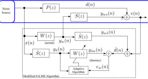
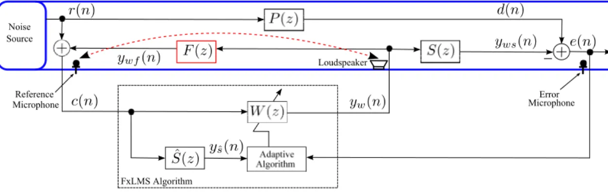
In ANC systems, the anti-noise signal generated by the loudspeaker will not only propagate downstream to cancel the original noise at the summing junction but also radiate upstream and corrupt the reference signal. This is the well known feedback effect in ANC system. For stable operation of ANC system it is required to neutralize this feedback effect using the feedback path neutralization (FBPN) filter.

(33)

Reference Microphone Loudspeaker Error Microphone Noise Source FxLMS Algorithm

Figure 1.11: Block diagram of single channel feedforward ANC system with

feed-back coupling.

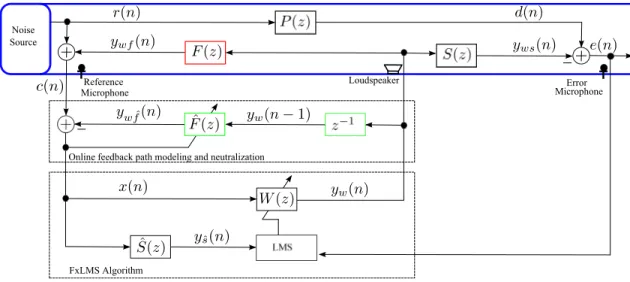
Need for feedback path neutralization: A block diagram of single channel feedforward ANC system with feedback coupling is shown in Fig. 1.11. Here F (z) is the feedback path transfer function from the output of W (z) to the reference mi-crophone. It includes the transfer functions of digital to analog converter (DAC), smoothing filter, power amplifier, loudspeaker, acoustic path from the loudspeaker to the reference microphone, pre-amplifier, anti-aliasing filter, and ADC [4]. From Fig. 1.11, the reference signal (corrupted) c(n) picked-up by the reference micro-phone is given by

c(n) = r(n) + ywf(n) = r(n) + (f (n)∗ yw(n)), (1.24) where r(n) is the original noise at the reference microphone, ywf(n) is the feedback coupling signal and represents the response of the ﬁlter F (z) corresponding to input yw(n). The objective of ANC system is to cancel the unwanted noise at the summing junction, i.e., to reduce the mean-square value of the error signal e(n). In order to see the eﬀect of feedback coupling on the error signal e(n), consider the z-transform of the error signal which is given by the expression

E(z) = P (z)R(z)− S(z) W (z)R(z)

(34)

Reference Microphone Loudspeaker Error Microphone Noise Source FxLMS Algorithm

Fixed feddback path neutralization

Figure 1.12: Block diagram of single channel feedforward ANC system with ﬁxed

feedback path neutralization.

It is clear from (1.25) that ANC system may become unstable if at some frequency

W (z)F (z) = 1. It is therefore necessary to neutralize the eﬀect of this feedback.

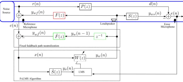
This neutralization can be done either by using the offline modeling or online modeling of F (z). The block diagram of single channel feedforward ANC system with fixed FBPN is shown in Fig. 1.12. The fixed FBPN filter ˆF (z) can be

obtained oﬄine, i.e., prior to operation of ANC system. Here z−1 is the inherent delay associated with the feedback path F (z). In order to neutralize the eﬀect of

F (z) it is required that ˆF (z)z−1 = F (z). The output y_{w ˆ}_f of ˆF (z) is subtracted from

the reference microphone signal, c(n), in order to generate the desired reference signal for W (z) as

x(n) = c(n)−y_{w ˆ}_f = x(n)−( ˆf (n)∗yw(n−1)) = x(n)−( ˆfT(n))x_{f (n),y}ˆ _w_(n₋₁₎(n−1)),

(1.26) where ˆf (n) is the impulse response of ˆF (z), ˆf (n) = [ ˆf0(n), ˆf1(n),· · · , ˆfLf−1(n)]

T is the impulse response coeﬃcient vector of ˆF (z) at time n, x_{f (n),y}ˆ _w_(n₋₁₎(n− 1) =

(35)

[yw(n− 1), yw(n− 2), · · · , yw(n− Lf)]T is the input signal vector of filter ˆF (z) with input yw(n − 1) at time n, and Lf is the tap-weight length of ˆF (z). The detail for the offline modeling of F (z) can be found in [4]. The procedure of offline modeling works well if the acoustic paths are time invariant, however in actual practice, the acoustic paths are time-varying, and hence online modeling is needed to track variations in feedback path. In this thesis, our focus will be the online feedback path modeling and neutralization (FBPMN). One of the basic online methods, proposed by Warnaka [12], is shown in Fig. 1.13. The purpose of adaptive FBPMN filter ˆF (z) is to cancel only the feedback part of the reference

microphone signal c(n) using yw(n) as the input excitation signal. However, as the signal yw(n) is highly correlated with the original unwanted noise r(n), therefore the ﬁlter ˆF (z) will adapt in such away as to incorrectly cancel the original primary

noise as well along with the feedback signal. Thus this structure will not allow ﬁlter W (z) to receive the signal r(n) at its input. This is the major problem with this structure and hence more sophisticated techniques, in which an additional auxiliary noise being modeled as white noise is injected for system identiﬁcation of unknown feedback path [4,5], are used for online FBPMN.

1.5 NLMS Adaptive Algorithm and Optimal

Ex-citation Signal

NLMS adaptive algorithm: It is shown in [22] that for LMS adaptive algorithm in Fig. 1.2, the convergence of the mean-square-error (MSE) is guaranteed if the step-size is selected within the bounds given by

(36)

Reference Microphone Loudspeaker _Error Microphone Noise Source FxLMS Algorithm

Online feedback path modeling and neutralization

Figure 1.13: Block diagram of single channel feedforward ANC system with online

feedback path modeling and neutralization.

where Px(n) is the power of input excitation signal of an adaptive algorithm. It is clear from (1.27) that in the case of LMS adaptive algorithm, the prior knowledge of the input signal power is required for the selection of step-size within the stability bounds. If the power of the input signal is time-varying, then the selection of a constant (ﬁxed) step-size may drive the algorithm unstable. The solution to the problem is to use normalized LMS (NLMS) algorithm [6]. The popularity of NLMS algorithm is due to its simplicity and automatic adjustment of initially selected step-size corresponding to varying input signal power. Considering Fig. 1.2 the weight update equation for NLMS algorithm is given by

ˆ w(n + 1) = ˆw(n) + µ e(n)xw(n),x(n)ˆ (n) xT ˆ w(n),x(n)(n)xw(n),x(n)ˆ (n) , (1.28) where ˆw(n) = [ ˆw0(n), ˆw1(n),· · · , ˆwLw−1(n)]

T _{is the impulse response coeﬃcient} vector of ˆW (z) at time n, and xw(n),x(n)ˆ (n) = [x(n), x(n− 1), · · · , x(n − Lw+ 1)]T is the input signal vector of ﬁlter ˆW (z) with input x(n) at time n. If the weight

error vector is deﬁned as ew(n) = w− ˆw(n), where w = [w0, w1,· · · , wLw−1]

(37)

Figure 1.14: Geometrical interpretation of (1.30).

the impulse response coeﬃcient vector of unknown system W (z), then using (1.28),

ew(n + 1) can be written as ew(n + 1) = ew(n)− µ e(n)xw(n),x(n)ˆ (n) xT ˆ w(n),x(n)(n)xw(n),x(n)ˆ (n) = ew(n)− µ e(n)xw(n),x(n)ˆ (n) ||xw(n),x(n)ˆ (n)||2 . (1.29) From Fig. 1.2, with v(n) = 0, the update equation for ew(n) can be written as

ew(n + 1) = ew(n)−µ (w− ˆw(n))T xw(n),x(n)ˆ (n) ||xw(n),x(n)ˆ (n)|| xw(n),x(n)ˆ (n) ||xw(n),x(n)ˆ (n)|| = ew(n)−µe∥w(n), (1.30) where xw(n),x(n)ˆ (n)

||xw(n),x(n)ˆ (n)|| is a unit vector, and e

∥

w(n) is the component of vector ew(n) parallel to input vector xw(n),x(n)ˆ (n). The geometrical interpretation of (1.30) is

shown in Fig. 1.14. It is clear from Fig. 1.14 that the e∥w(n) component of ew(n) can contribute to its desirable reduction for

0 < µ < 2, (1.31)

where the range of step-size µ in (1.31) is the stability criterion for NLMS algo-rithm. The convergence of NLMS algorithm degrades for correlated input signal having large eigenvalue ratio [8]. Therefore, for better convergence of NLMS algo-rithm the selection of the optimal input excitation signal is very important.

(38)

Optimal excitation signal: From the theory of signal processing, it is known that the cross-correlation Rxy(n) between input x(n) and output y(n) of a linear ﬁlter is equal to the convolution of the autocorrelation of input Rxx(n) with system impulse response w(n), and is computed as

Rxy(n) = Rxx(n)∗ w(n). (1.32) For input excitation signal with impulse like autocorrelation function, i.e., Rxx(n) =

δ(n), the cross-correlation is the measure of the impulse response of system.

There-fore it is required that the input excitation signal must have the ideal impulse like autocorrelation function. The selection of the excitation signal for adaptive filter depends upon specific applications. When the designer is provided with a choice for the selection of input excitation signal, one choice could be the random white noise due to having wide range of frequency components and flat power spectrum over the entire frequency range. However, it is shown in [23]-[29] that the optimal excitation signal that shows high energy efficiency and improves the convergence of NLMS algorithm is a deterministic Perfect-Periodic-Sequences (PPSEQ) having period equal to the tap-weight length of adaptive filter and shows desired autocor-relation properties given by

Rxx(i) = L∑w−1 n=0 x(n)x(n + i) =      Ex (if i = 0 (mod Lw)) 0 (Otherwise) , (1.33)

where Ex is the energy of one period of the signal. Furthermore, in [30] it is shown that in the practical set-ups, due to the presence of nonlinearities, the property of high energy eﬃciency associated with PPSEQ can not be achieved. Therefore a new class of excitation signals referred as perfect-sweeps are introduced in [31]. The perfect-sweep signal is a time-stretched pulse [32] having the desired properties of

(39)

PPSEQ along with high immunity against distortions. For perfect-sweep signal, the general construction formula is given

P (k) =      exp(−j4mπk_L2 2 w ) (0≤ k ≤ Lw 2 ) P (Lw − k) (L₂w < k < Lw) , (1.34)

where k is the frequency index, Lw is the length of one period of signal, m de-termines the stretch of the time-stretched pulse, and P (k) represents the complex conjugate of P (k). The signal in the time domain is obtained by taking the inverse transform of P (k).

The geometric interpretation of NLMS algorithm in Fig. 1.14 shows that for

µ = 1 the parallel component e∥w(n) can be completely eliminated. Similarly all the Lw components of ew(n) can be compensated if the Lw consecutive input vectors to an adaptive ﬁlter ˆW (z) are orthogonal. In the case of random white

noise input excitation signal x(n), the Lw consecutive input vectors of inﬁnite length, denoted by x′_w(n),x(n)_ˆ (n), x′_w(n),x(n_ˆ ₋₁₎(n−1), · · · , x′_w(n),x(n_ˆ _−L

w+1)(n−Lw+1),

are orthogonal in the inﬁnite vector space. The vectors of length Lw, denoted by xw(n),x(n)ˆ (n), xw(n),x(nˆ −1)(n − 1), · · · , xw(n),x(nˆ −Lw+1)(n − Lw + 1), represents,

respectively, the projection of vectors denoted by x′_w(n),x(n)_ˆ (n), x′_w(n),x(n_ˆ ₋₁₎(n − 1),· · · , x′_w(n),x(n_ˆ _−L

w+1)(n − Lw + 1) onto the Lw dimensional vector space. For

the projected vectors in the Lw dimensional space the orthogonality is not guaran-teed, therefore it can be concluded that the random white noise is not an optimal excitation signal [26]. For the PPSEQ, it is clear from the autocorrelation property given in (1.33) that the Lw consecutive vectors are orthogonal and thus represents the optimal excitation signal. As stated earlier, in practical set-ups the presence of nonlinear distortion can limit the performance of PPSEQ. Therefore, in this case the perfect-sweep excitation signal, having all the desired properties of PPSEQ

(40)

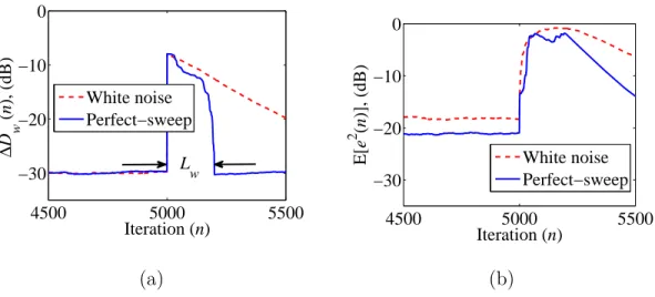
4500 5000 5500 −30 −20 −10 0 Iteration (n) ∆ D w ( n ), (dB) White noise Perfect−sweep L w (a) 4500 5000 5500 −30 −20 −10 0 Iteration (n) E[ e 2 (n )], (dB) White noise Perfect−sweep (b)

Figure 1.15: Simulation results for Case 1 (SNR=30 dB): (a) Relative modeling

error, ∆Dw(n)(dB), (b) Mean-square-error, MSE (dB).

and shows improved performance with nonlinear distortion, can be the best choice for system identiﬁcation [33]. The simulation results of NLMS algorithm based system identiﬁcation for Case 1: with SNR=∞ dB, i.e., v(n) = 0, and Case 2: with SNR=30 dB, are shown, respectively, in Fig. 1.15 and Fig. 1.16. The perfor-mance comparison is carried out on the basis of following perforperfor-mance measures.

• Relative modeling error ∆Dw(n) in dB, being deﬁned as

∆Dw(n) = 10log10

||w(n) − ˆw(n)||2

||w(n)||2 dB. (1.35)

• MSE E[e2_{(n)] in dB.}

For the simulation results, the data for the unknown system is selected from [4], the length of unknown system and adaptive ﬁlters is selected as Lw = 200. The acoustic paths are perturbed in the middle of simulation, and all the results are averaged over 10 independent realizations. The rest of the simulation parameters are the

(41)

0 5000 10000 −300 −200 −100 0 Iteration (n) ∆ D w ( n ), (dB) _{White noise} Perfect−sweep (a) 0 5000 10000 −300 −200 −100 0 Iteration (n) E[ e 2 (n )], (dB) White noise Perfect−sweep (b)

Figure 1.16: Simulation results for Case 2 (SNR=_{∞ dB i.e v(n) = 0): (a) Relative}

modeling error, ∆Dw(n)(dB), (b) Mean-square-error, MSE (dB).

same as in [33]. It is clear from Fig.1.15(a) and Fig. 1.16(a) that with perfect-sweep input excitation signal the system can be identiﬁed in Lw iterations, while the convergence of the system with white noise input is slow and requires more than

Lwiterations. The curves for the MSE in Case 1 and Case 2, respectively, are shown in Fig.1.15(b) and Fig. 1.16(b). From these curves it is clear that identiﬁcation with perfect-sweep excitation signal results in lower steady-state MSE.

1.6 Need of Gain Scheduling of Auxiliary Noise

For stable operation of ANC systems, the estimates (identiﬁcation) of the unknown secondary path and the feedback path are required [4]. In order to obtain these estimates, an additional auxiliary noise is required to be injected into the ANC system [21]. On one hand, the injection of auxiliary noise into the ANC system is useful to get the required estimates of secondary and feedback path, but on the other hand, the injection of auxiliary noise contributes to the residual error (which

(42)

we want to minimize) and will degrade the noise-reduction-performance (NRP) of ANC system. The solution, for improving the NRP, is to use gain scheduling strategy to vary the variance of auxiliary noise. At the start (when ANC system is far from steady-state), it is required that the gain scheduling strategy must allow the auxiliary noise to have large variance to obtain the better estimates of the unknown secondary and feedback paths. At the steady-state, it is required that the gain scheduling strategy must reduce the variance of auxiliary noise to a small value to improve the NRP of ANC system.

From [33], it can be concluded that the perfect sweep signal can be the optimal auxiliary input excitation signal for system identiﬁcation purpose. However, in ANC literature [4,5] the most common choice of auxiliary input excitation signal for system identiﬁcation is the WGN. In this thesis the WGN will be used as an auxiliary noise signal for OSPM and online FBPMN.

1.7 Summary

In this introductory chapter, the underlying physical principle used for acoustic noise cancellation is explained. In order to show the importance of this idea, some practical examples where this idea can be employed are given, and the brief overview of the most popular application of ANC system for acoustic duct is pro-vided.

The idea of direct and indirect system identification is discussed, and the deriva-tion of the most popular adaptive FxLMS algorithm for ANC systems is described. The idea of MFxLMS algorithm to convert the problem of indirect system identi-fication in ANC system to a problem of direct system identiidenti-fication is explained.

(43)

are discussed. A brief overview of some basic techniques used for OSPM and online FBPMN is given, while the detail will be given in the coming chapters.

The role of the input excitation signal for NLMS algorithm based identiﬁcation of an unknown system is explained, and it is found that perfect-sweep excitation signal is the optimal choice. Finally the need of gain scheduling of auxiliary noise has been discussed.

In the following chapter 2 and chapter 3 the focus is on OSPM. In chapter 2, the existing methods for OSPM without gain scheduling (auxiliary noise with fixed variance is used in all operating conditions) will be discussed. In chapter 3, the existing methods of OSPM using gain scheduling of auxiliary noise are explained. In addition to this, new strategies for gain scheduling of auxiliary noise are proposed. In existing methods, the gain is varied based on the power of residual error signal which carries information only about the convergence status of ANC system. In the proposed methods the gain is varied based on the power of error signal of SPM filter. This is more desirable way of controlling the gain because the power of error signal of SPM filter carries information about the convergence status of both the ANC system and SPM filter. The simulations are carried out to show that the proposed gain scheduling strategies improve both the modeling accuracy of SPM filter and the NRP of overall ANC systems.

In chapter 4, the issue of online FBPMN with and without gain scheduling of auxiliary noise is explained. In the ﬁrst part of this chapter, the existing meth-ods for online FBPMN without gain scheduling are discussed. A new structure is proposed that combines the good features of the existing structures to better neutralize the eﬀect of the feedback coupling and to improve the convergence of ANC system. In the second part of this chapter, a gain scheduling strategy is

(44)

proposed, for online FBPMN, to improve the NRP of ANC system. In addition to this, a self-tuned ANP scheduling strategy with matching step-size for FBPMN ﬁlter is also proposed that requires no tuning parameters and further improves the NRP of ANC systems.

In chapter 5, the concluding remarks and the future research directions are given.

(45)

Chapter 2 Online Secondary Path Modeling

Without Gain Scheduling

With the invention of high speed digital hardware and the development of adaptive signal processing algorithms, the field of active noise control (ANC) has found a great attention of the researchers since the last three decades. The basic crux of ANC system is the principle of superposition in which the acoustic waves of the original unwanted noise interfere destructively with the acoustic waves gen-erated by the combination of ANC filter followed by the secondary path. In order for the ANC systems to converge properly, it is necessary to compensate for the effects of the secondary path. For some applications the secondary path can be estimated offline, i.e., prior to the operation of an ANC system. However, for most of the practical applications the secondary path is time-varying and therefore

(46)

on-line secondary path modeling (OSPM) is required, i.e., when ANC system is in operation.

OSPM with higher modeling accuracy and faster convergence is desirable in ANC systems to ensure large stability margins. There are two different approaches for OSPM in ANC systems. The first approach models the secondary path using the output of ANC filter W (z) as an input excitation signal of secondary path modeling (SPM) filter. The second approach involves injection of additional ran-dom noise into the output of W (z), and utilizes a system identification method to model the secondary path. The additional noise injected is uncorrelated with the original unwanted noise. The comparison of the two approaches for OSPM can be found in [34], where it is concluded that the second approach is superior to the first one when compared in terms of convergence rate, and speed of response to changes in original unwanted noise. In this chapter, the use of second approach is considered for OSPM, however additional noise with fixed variance is injected, i.e., no gain scheduling is used.

In the first part of this chapter, various existing methods using filtered-x-LMS (FxLMS) adaptive algorithm for ANC filter W (z), are briefly explained for OSPM. In the second part of this chapter, a method using modified-filtered-x-LMS (MFxLMS) adaptive algorithm [5] for ANC filter W (z), is explained for OSPM. In this second part, a new computationally efficient MFxLMS (CEMFxLMS) al-gorithm is proposed. The proposed structure is simple than the original structure using MFxLMS algorithm for OSPM. The performance of the MFxLMS algorithm based ANC system with OSPM is compared with the proposed CEMFxLMS al-gorithm through computer simulations. We will see that the performance of the proposed CEMFxLMS algorithm is same as obtained with the original MFxLMS

(47)

al-gorithm. However, CEMFxLMS algorithm has lower computational requirements compared to MFxLMS algorithm.

2.1 FxLMS Algorithm Based ANC Systems

For OSPM without gain scheduling an additional white Gaussian noise (WGN), here after called as auxiliary noise, with fixed variance is injected in all operat-ing conditions. In this section a brief overview of Eriksson’s method [21], Kuo’s method [35], Bao’s method [36], Zhang’s method [37], and Akhtar’s method [38] is given. This section also describes a variable step-size (VSS) method [39] for OSPM without gain scheduling. In all these methods FxLMS algorithm is used for ANC filter W (z), and auxiliary noise with fixed variance is injected for SPM filter. The performance of all previously mentioned methods are compared through the simulation results, and it is found that the VSS approach in [39] outperforms in terms of improving the modeling accuracy of SPM filter compared to other existing methods.

2.1.1 Eriksson’s Method

The block diagram of Eriksson’s structure [21] for OSPM is shown in Fig. 2.1. Here G(n) = 1 shows that no gain scheduling is used, and auxiliary noise with ﬁxed variance is injected in all operating conditions. From Fig. 2.1, the error signal is given by

e(n) = [d(n)− yws(n)] + vs(n). (2.1)

In Eriksson’s method, the signal e(n) acts both as an error signal for W (z) and as a desired response of SPM ﬁlter. The following are the problems associated with the Eriksson’s structure.

(48)

Noise Source

Generator

Figure 2.1: Block diagram of Eriksson’s method for ANC systems with online

secondary path modeling [21].

• In e(n), the first term in square brackets acts as an interference for SPM filter, and thus may affect the convergence of SPM filter.

• The last term vs(n) in e(n) acts as an interference for ANC ﬁlter W (z), thus aﬀects its convergence.

2.1.2 Kuo’s Method

The block diagram of Kuo’s structure [35] for OSPM is shown in Fig. 2.2. In addition to ANC filter W (z) and SPM filter ˆS(z), a third adaptive filter K(z)

(termed as the prediction error filter) is used to remove the interference from the desired response of the ˆS(z). Here, the error signal ek(n) of adaptive filter K(z) acts as a desired response of SPM filter and is computed as

ek(n) = e(n)− yk(n), (2.2) where yk(n) is the output of prediction error ﬁlter K(z), and is computed as

(49)

Noise Source

Generator

Predictor

Figure 2.2: Block diagram of Kuo’s method for ANC systems with online secondary

path modeling [35].

where k(n) is the impulse response of K(z), ∆ is the delay, e(n− ∆) is the de-layed version of e(n), k(n) = [k0(n), k1(n),· · · , kLk−1(n)]

T _{is the impulse response} coeﬃcient vector of K(z) at time n, and xk(n),e(n−∆)(n− ∆) = [e(n − ∆), e(n − ∆− 1), · · · , e(n − ∆ − Lk+ 1)]T is the input signal vector of ﬁlter K(z) with input

e(n− ∆) at time n.

From the theory of adaptive ﬁltering, it is known that the adaptive ﬁlter output converges to that part of its desired response which is correlated with the input excitation signal. It is shown in [35], for ∆≥ Ls the term vs(n− ∆) in e(n − ∆) becomes uncorrelated with the term vs(n) in e(n). As a result, at the steady-state,

yk(n) → [d(n) − yws(n)], and ek(n) → vs(n). Thus the Kuo’s structure is capable of removing the interference term [d(n)− yws(n)] from the desired response, ek(n),

A Study on Gain Scheduling of Auxiliary Noise for Online Secondary and Feedback Path Modeling in Active Noise Control Systems