Branch-and-Bound Approach for a Stochastic Production Planning Problem with Capacity Constraints

Journal of the Operations Research Society of Japan

Vo!. 31, No. 4, December 1988

BRANCH-AND-BOUND APPROACH FOR

A

STOCHASTIC PRODUCTION PLANNING PROBLEM

WITH CAPACITY CONSTRAINTS

Chang Sup Sung Young Jin Lee Korea Advanced Institute of Science and Technology

(Received August 15, 1987; Revised March ID, 1988)

Abstract A stochastic production planning problem with a fmite number of planning periods is analyzed where cumulative demands up to each period are independent random variables with continuous probability distributions. In the problem, backlogging is permitted and production is restricted by its capacity. Dynamic but linear costs of inventory holding and backlogging, and of production with setup charge are considered. A branch·and-bound algorithm is developed to find an optimal plan within fmite searching steps, and its computational effectiveness is evaiuated.

1. I ntroducti on

This paper considers a production planning problem with known stochastic demands where the planning horizon is composed of a finite number of planning periods and cumulative demands up to each period have a continuous probability distribution. Capacity restrictions are imposed on production. and unsatis-fied demands are backlogged. Furthermore. dynamic but linear costs of inventory holding and backlogging. and of production with setup charge are included. The production problem can then be interpreted as in a similar form to a stochastic programming problem with simple recourse (Ziemba [12]). In fact. the stochastic production problem shall be transformed to an equivalent deterministic problem from which an optimal solution to the original problem ~s obtained.

The equivalent deterministic problem has an objective function which is neither convex nor concave. Rather. it is a mixture of convex and concave functions which makes it difficult to solve the problem by using usual convex programming or concave programming algorithms. Therefore. this paper suggests

a branch-and-bound algoritlun which can determine an optimal solution to the deterministic problem within finite searching steps.

The branch-and-bound algoritlun is exploited based on the concept of convex envelope (Falk and Hoffman [5]). That is, by transforming the concave part of the objective function into an underestimated linear approximate, an ~nderestimated convex objective function, so-called, convex envelope, is derived. The convex envelope and its associated solution space are then partitioned so as to constitute subproblems. Each of the subproblems leads to construct a sub-tree in the branch-and-bound algoritlun for which branching rules and bounding schemes are mechanized to make an efficient optimal solu-tion search for the equivalent deterministic problem (and accordingly for the original problem) within finite steps.

Hadley [6] has discussed a similar problem in a dynamic programming formulation but without incorporating any production capacity restriction. Nevison and Burstein [9] have treated a stochastic production problem with stochastic lead times of demand. They permitted inventory backloggings but did not consider any production capacity. Bitran and Yanasse [3] have con'-sidered deterministic approximations to stochastic production planning problems where cumulative demand quanti ties are random variables and no backlogging is allowed.

In section 2, the stochastic production planning problem is formulated in a mathematical model, and its equivalent deterministic problem is derived. In section 3, a branch-and-bound algoritrm is developed. In section 4, a convex programming algorithm is introduced for subproblems corresponding to each sub-tree of the branch-and-bound algoritlun. In section 5, the computa-tional performance of the algoritlun is evaluated on various criteria by use of its test results on a number of numerical examples. In section 6, concluding remarks are presented.

2. Model Formulation

(i) (ii) (iii) (i v) (v)

For the stochastic production problem, the followings are assumed; The cumulative demand up to each period has a known continuous proba-bility distribution.

Production at each period is restricted within its capacity. Backloggings are permitted.

Setup charge is imposed on each production, and costs of production, of on-hand inventory holding, and of inventory backlogging are linear. Planning horizon of periods is finite.

534 C~SungandY.~Lee

With the assumptions (i)-(v), the stochastic production problem (sPp) is formulated as follows; (SPp) Min. where T x t d t It + It

-It Ut Kt et h+ t h t c5 (y) E [.] F(x)

o

:5 X_t :5 Ut ' + It = It - It ' + -x

t ' It' It ~ 0 for all t=l, ... ~T,

planning horizon,

amount of production at period t, nonnegative random demand for period t, amount of inventory at the end of period t, on-hand inventory at the end of period t, backlogged inventory at the end of period t, production capacity at period t,

setup cost at period t,

unit production cost at period t,

inventory holding cost per unit at period t, inventory backlogging cost per unit at period t,

1 if y > 0, or 0 otherwise,

operation of expectation.

In the model, without loss of generality, it is assumed that the starting inventory IO=O.

+

-It and It are restated as follows; t (1) _It + max{O,

_L

(x. -d .) } i=l ~ ~ t (2) _It max{O,

L

(d.-x.)} i=l ~ ~

+

-Substituting It and It in (sPp) with (1) and (2), respectively, the following

problem (SP) is obtained as an equivalent formulation of (SPp):

(Sp) Min. (3) s. t . (4) t + h~max{O.

I

(d.-x.)}]] i=l ~ ~

o

~ x

t ~ Ut' for all t=l •...• T.

F(x) in (3) can be rewritten T t F(x)

I

[{KtC(Xt)+ctx_t} + E[h;max{O.

I

(x.-d.)} t=l i=l ~ ~ t + h~max{O,

I

(d.-x.)}]] i=l ~ ~ Letting Zt

=

(x₁'···.x_{t ).} pt(x_t)

=

_{KtC(Xt)+ctxt •} and if follows that where F(x)

=

p(x) + Q(x) p(X) T

I

pt(x_t) and Q(x) t=l

Let g (0) be the probability density function of the cumulative demand up t t

to period t.

I

d .• t=l •...• T. Then an explicit expression of Q(x) is easily i=l ~

derived in terms of gt(o),

t

(5 )

I

x.

i=l ~ t t t

(h;+h~)f

(

I

x·-y)gt(y)dy +

h~[E(

I

d.)-

I

x.] •

o

i=l ~ i=l ~ i=l ~

for all t=l, ...• T.

Y t

In (5). the term f (Yt-y)gt(y)dy represents the expected number of

536 c.S.SungandY.~Lee

on-hand inventory at period t, which may characterize whether or not the ex-pected inventory cost (incurred by both holding and backlogging), Qt(Zt)' at period t can be interpreted as a deterministic function. Since the cumulative

t production up to period t, Y

t= _i=l

L

x., _~ is finitely bounded above for all t=l, Y

t

... ,T, the integral

f

(Yt-y)gt(y)dy exists for all Y

t, t=l, ... ,T.

o

Recall that in problem (SP), the objective function F(x) is decomposed into the production cost p(x) and the expected inventory cost Q(x). And the random variables d

t, t=l, ... ,T, are related only to the function Q(x). Thus,

by representing Q(x) in the explicit form of (5) which is not haunted by the random variables d

t, t=l, ... ,T, the overall cost function F(x) takes a

deter-ministic form. This leads to the following equivalent deterministic problem (EDP) of (SPp).

(EDP)

(6) Min. F(x)

=

p(x) + Q(x)

s.t. 0 ~ x_t ~ Ut' for all t=l, ... ,T,

where Q(x) is defined as in (5).

If demands in each period are independent Gamma or normally distributed random variables, then the cumulative demands up to each period are also Gamma or normally distributed, respectively. Thus, from these distributions, the deterministic functions F(x) as required in (6) can analytically be derived from the well-known Gamma-Poisson relationship or by integrating by parts, respectively.

3.

Branch-and-Bound Algorithm

In order to formulate a solution algorithm, it shall first be proved that the expected inventory cost function Q(x) is convex. Let Z denote the solution set of problem (EDP);

z {x

I

0 5 x_t 5 Ut' t=l, ... ,T } .

Then z is a compact convex set.

Theorem 3.1.

The expected inventory cost function Q(x) in (5) ~s convex for all x E Z.

Y t

The integral term

f

(Yt-y)g (y)dy in (5) can easily be shown as

o

t

Proof:

p .89) for all t=1, ... ,T. It follows that Q(x) is the summation of convex functions for all x £

z.

This completes the proof.

On the other hand. the expected production cost function p(x) is observed as a concave function for all x £ Z, since it is the summation of concave functions P (x ) on Z, t=1, ... ,T.

t t:

Now let w(x) be a linear underestima.ting function of p(x) for all x £ z; T

(7) W(x)

=

L

Wt(x_t) t=1 where

for all x=(x₁ •... ,x_T) £ Z and t=1, ... ,T.

Then, according to Falk and Hoffman [5], w(x) is a convex envelope of p(x), which is characterized as in the next theorem.

Theorem

3.2. Let w(x) be defined as in (7). Then w(x) is a convex envelope of p(x) defined on the convex set z, which satisfies the conditions

(i) W is a convex function defined over the convex set Z where W(x) ~

p(x) for all x £ Z, and

(ii) if H is any convex function defined over Z such that H(x) S p(x) for all x £ z,

then H(x) ~ W(x) for all x £ Z.

Proof:

The convexity of w(x) directly follows because w(x) is a linear function for all x £ Z. It also holds that

W(x) - p(x)

T

L

[Kt{Xt/U_t - O(x

t)}] ~ 0 ,

t=1

since 0 ~ x_t ~ Ut for all t=1, ... ,T. Therefore, the condition (i) ~s satis-fied. Now, for all t=1, ...

,T,

Moreover, pt(x

t) is concave for all Xt' 0 ~ xt ~ Ut' Thus, it is evident that the linear function Wt(x

t) satisfies the result of (ii). This completes the proof.

Let f(x) = W(x) + Q(x), where Q(x) is defined as in (5). From Theorem 3.2, it can easily be verified that f(x) is a convex envelope of F(x). There-fore, by substi.tuting f(x) for F(x) in (EDP), the following convex programming problem (cp) is derived:

538

c.

S. Sung and Y. J. Lee

(cp)

Min. f(x)

s.t. xe:Z

Moreover, solutions of (EDP) and (Cp) lead to the following relationship.

Theorem 3.3. Let x and x

*

be the optimal solutions of (Cp) and (EDP), respectively. Then, it follows that

,

*

f(x ) $ F(x )

Proof: By definition, for all x e: Z, f(x) $ F(x). Therefore

,

*

*

f(x ) , f(x ) S F(x ) ,

*

'

since x e: Z and min{f(x) Ix e: Z}

=

f(x ). This completes the proof. Now, our branch-and-bound algorithm is described. Soland [11] has

proposed a branch-and-bound algorithm for an optimal facility location problem with concave costs. Recently, Erenguc and Tufekci [4] presented an extended branch-and-bound algorithm for a lot sizing problem with deterministic demands, from which our algorithm is derived similarly.

°

1

Let the nodes of the branch-and-bound tree be denoted by N • N , .••• with NO representing the initial node. Each node

~

represents a subproblem with solution space zk defined as a subset of Z and its corresponding objective function

~

which is a convex envelope of F on zk. Each zk is specified as follows:

that

where

zk

=

{xIL~ ~

x

t

~

0:,

t=l, •.. ,T} for all k (k=0,1,2, .•. ) such (i) (ii) (iii) e: k and k i f t e: Ak, Lt e: Ut Ut' k Lt

~

=

0, if t e: B , k and Lk t

°

and

0:

Ut' if t k e: J • {l, ..• ,T},

the set of pre'-specified production periods,

the set of pre-specified non-production periods,

k k

I - A

U

B

=

the set of undecided periods, and

an arbitrary small positive value provided initially so as to indicate each possible production setup.

At the k-th stage during the algoritlun, a node, say,

wr

is selected to provide a least lower bound value among a.ll current candidate nodes for further branching. Then at the next stage k=k+1, the tree branches from the node

wr

2k-1 2 k . 2k-1

to two new nodes N a n d N correspondl.ng to the solution spaces

z

and z2k, respectively, such that z2k-1 Uz2k

=

zr. In the way, the algoritlun

°

1 m

generates a sequence of feasible points 1n Z, (x , x , ... , x , ... ) (m=O, 1, 2, ... ), where xm is an optimal solution of subproblem at node~. Since xm is a feasible point in z, F(xm) becomes an upper bound of F(x) for subproblem at node ~.

Denote by UB(~) the upper bound attained at node ~, so that UB(~) ,.

F(xk). Let UBk

F = min{F(x i

)li=O,l, ... ,k} and UBk = xh for xh E z, where UBk

, x F

F(xh). UBk is an upper bound on the optimal solution value of problem (EDI'),

F

and UBk is the best solution of (EDP) found over nodes NO through Nk

x

Let

LB(~)

denote a lower bound of the optimal value of F defined on zk. It is now shown how the lower bound

LB(~)

is calculated. Let the convex envelope of F(x) associated with zk be denoted by

~(x)

which satisfies

(8)

~(x) = ~(x)

+ Q(x) where

~(x)

T

L

>{(x

_t ) and t=l

~(Xt)

-

I

Kt _{+ CtX if t} k t , E A 0, if t E B k and (c t + Kt/Ut)Xt, if t k E J for all t=l, ... ,T.

For k=O, let AO and BO be null sets so that JO

=

I.

From the result of Theorem 3.3, substituting f(x) and

z

with

~(x)

and zk, respectively, leads to

~(xk)

$ F(X*), where

~(xk) = min{~(x) Ix E zk} and F(X*) = min{F(x) Ix E zk} .

Therefore, a lower bound of the ml.nl.mum of F(x) defined on zk is deter-mined such that

LB(~)

=

~(xk),

where xk solves the following subproblem

(Cpk) at node ~; (cpk)

Min.

~(x)

540

c.

S. Sung and Y. J. Lee

Now, suppose that, at the end of stage k during the branch-and-bound algorithm, an intermediate node Nr is to be branched further. This will only be the case in which LB(Nr) < UB;k, where the last numbered node at the stage

is NZk. Let xr be the solution to problem (Cpr) at the corresponding node

~.

Choose any t E Jr, called tr, which maximizes the difference (9)

Then, at the (k+l)st stage, the node ~ is branched to generate two nodes

Zk+l Zk+Z . Zk+l Zk+Z . Zk+l

N a n d N accordLng to Z and Z ,respectLvely, where Z and zZk+Z differ from zr only at the period tr which satisfies (9). Theorem 3.4 underlies the determination of such a period tr.

Theorem 3.4.

Assume that NZ(k-l) is the last numbered node at the start

of the k-th stage during the branch-and-bound algorithm and Nr is one of the intermediate nodes such that

LB(~)

< UB;(k-l). Then there exists at least one period t such that

(i) (H) (Hi) r t E J r

o

~ x_t < Ut ' and r Kt (l - Xt/Ut) > 0

Proof:

Since Nr is an intermediate node, Jr has at least one element. Otherwise, it is an already fathomed node which cannot be branched from. Thus, we have so that (10) Moreover, [p(xr) + Q(xr) p(xr ) _ wr(xr) r

For all t=l, ... ,T, from the definition of Wt(x) Ln (8), it follows

that ( 0, i f r _Br pt (xr) t E A _U r r (11)

-

W t (x ) _{= K} t(l r if r - xt/ut ), t E J

Since F(Xr) - r(xr) > 0 from (10), it follows that there exists at least one period t which satisfies the conditions (i)-(iii). This completes the proof.

Based on the results of Theorem 3.4, at the k-th stage ZI is divided into

Zk-l Zk

two subsets Z and Z . These subsets are specified by their index sets Zk-j BZk- 1 d A Zk d Zk . I

A and an an B ,respectl.ve y, such that (i) AZk-1 = AI U {tr} and BZk-1 = BI, and

(H) AZk = Ar and BZk = BI U {tr} , where

As the algori thm proceeds, a lis t of nodes that need be further branched from is maintained. This list is called the candidate list. Now, the branch-and-bound algorithm is formulated as in Steps (i), (ii), and (iii).

Step (i). Let k=O=p. Set NO with zO=Z, and

.

° ° °

° °

gl.Ve LB(N )=f (x ), UB(N )=F(x ), Add NO to the candidate list. Go

° °

A =B =cjl. Solve

° °

UBF=UB(N ), and to step (iH). fO(x) for xO to

° °

UB =x x

Step (ii). If there is no node in the candidate list, then terminate and obtain an optimal solution of (EDP). Otherwise, find r such that

LB(~)

is the minimum of

LB(~)

among all intermediate nodes

~

in the candidate list. If

LB(~)

;:: UBZk, then terminate and obtain

Zk F

an optimal solution of (EDP), UB Otherwise, set p=I and go to x

step (Hi).

P

n-l

Step (iii). Let k=k+l. Branch from node N to generate two new nodes N

Zk . Zk-l Zk

and N added to the candidate list. Fl.nd LB(N ) and LB(N ).

Zk Zk

Update UB and UB

F x

Step (iv). (Fathoming tests)

Step (iv-a). (Completeness test)

Fathom a node Ni in the candidate list such that Ai U Bi I. Step (iv-b). (Bound test)

Fathom a node Ni such that

LB(~)

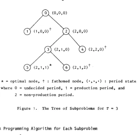
;:: UB;k. Go to Step (ii).

The above branch-and-bound algorithm is illustrated by Figure 1 depicting the entire tree of subproblems for T=3. It should be clear that, if the algorithm terminates at stage k, then UB;k (the last numbered node NZk) is an optimal solution of (EDP). The algorithm terminates within finite steps, since at most (ZT+ 1 ) nodes are necessary to be examined for the optimal solu-tion.

542 C S. Sung and Y. J. Lee

°

(0,0,0) 0<:2,1,1)* 6 (2,0,0) t (2,2,0) t (2,1,2)

*

= optimal node, t : fathomed node, ( " " . ) : period state, where

°

2

undecided period, 1

=

production period, and non-production period.

Figure 1. The Tree of Subproblems for T ~ 3

4. Convex Programming Algorithm for Each Subproblem

T each node

~

in the branch-and-bound algorithm, the subptoblem (Cpk) LS

corresponded. Recall that

Min.

~(X) = ~(x)

+ Q(x)

S. t.

By definition, wk(x) is a continuous differentiable convex function k

defined on Z , and Q(x) in (5) is also a continuous differentiable function for all x E

zk.

Let

V~(x)

=

(V~(x),

...

,V~(x»

where

V~(x)

=

a~(x)/axi'

i=l, .•. ,T. Then it follows that

V~(x) = a~(x)/ax.

+ aQ(x)/ax. for all

J. J. J. i =1, ••• , T, where

1

c i ' if i E Ak

a~(x)/ax.

0, if i E B k and J. c.+K./U., if i E J k J. .1 J. and

aQ(x)/ax. is given in Theorem 4.1.

where

Theorem 4.1.

For all i=l, ••• ,T,

T

aQ(x)/ax_i =

I.[(h;+h;)Gt(Yt)-h~]

,

t=~

t

G_t(') is the distribution function of

I

d., for all t=I, ... ,T. i=1 ~

Proof:

Based on the differentiation rule of a definite integral with respect to a parameter Y

t (Heyman and Sobel [8], pp.518-519),

T

aQ(x)/ax.

=

I

aQt(Zt)/ax . .

~ t=1 ~

+ - Y_t

aQt(Zt)/ax_i = a[(ht+ht){J (yt-y)gt(y)dy}

o

if t=I, ... ,i-I and

if t=i, ... ,T.

This completes the proof.

Since (cpk) is a usual convex programming problem, general solution algo-rithms can be adapted for the convex programming. In specific, the algorithm of Frank and Wolfe [2] is employed here to solve the subproblem (Cpk), since it guarantees generally the convergence of the solution to the Kuhn-Tucker point. The Frank-Wolfe algorithm is given below where for brevity of expres-sion the stage index k is deleted:

Step O. Find an initial feasible point x in

z.

Step I. Calculate Vf(x) and let for all t=I, ... ,T,

y

=

t ( Ut' if Vft(x)<O , Lt' if Vft(x)~O .

*

Step 2. Find the scalar value \ where

*

\ argmin{f(h + (I-\)y) IOS:\S:I}

*

*

*

*

Step 3. Let y = \ x + (1-\ )y. I f If(y )-f(x)

I

s: E, then terminate.

*

Otherwise, update x

=

y and go to Step I.

*

In Step 3, the scalar value \ can be found by using any available one-dimensional search method, for example, the well-known Golden Section method or the Newton method. In this paper, an efficient search method, so-called, Brent's method, is rather employed which intends parabolic interpolation to

544

c.

S. Sung and Y. J. Lee

*

find the optimal value of scalar A (Press et al. [10]).

For each subproblem (Cpk), an initial feasible solution can easily be provided, since the solution set zk is defined over the ranges

L~ ~

x

t

~ ~

for all t=l, ... ,T, and so any x

t value can be selected as the initial solution

k k

between Lt and Ut' Thus, incorporating the algorithm of Frank and Wolfe [2]

o

1

into the branch-and-bound algorithm, a sequence of feasible points (x , x , ... , xk, ... ) (k=O, 1,2, ... ) is obtained where xk is an optimal solution at each subproblem at

node~.

This leads to an optimal solution of (EDP) by following the whole procedure of the branch-and-bound algorithm over such all possible nodes.

5. Computational Effectiveness of the Branch-and-Bound Algorithm

To examine the effectiveness of the proposed branch-and-bound algorithm a number of numerical examples are generated by varying the problem parameters. And then by solving the problems, the computational performance is evaluated on various criteria. This computational experiment is designed based on the study of Baker et al. 's [1] where they have treated a similar problem with deterministic demands, stationary costs and capacities.

(a) Generation of numerical examples

In order to draw valid conclusions, a number of variations on problem parameters are considered. The problem parameters include demand pattern, planning horizon, cost variations in ratio, and capacity level.

For the demand pattern, two cases, stationary and seasonal demands, are considered. For the stationary demand, the expected value of demand at each period t, D

t

=

E[dt], is generated from the uniform interval [100, 300] and 1/2

its variance is given as (Var(d

t

»

O.lDt. For the seasonal demand, the

demand is given:

(12) D

t = ) l + a-sin[2'rr(t+b/4)/b], t=l, ... ,T,

where

T planning horizon,

)l average demand during the planning horizon T,

a

=

amplitude of the seasonality, and b length of seasonal cycle, in periods.

For each test problem with a planning horizon T, the average demand )1 is generated from the uniform interval [100, 300]. Then with the fixed value of

equa-tion (12) at a

=

0.5~ and b

=

T. For this seasonal demand, the variance of demand at period t is given to increase 'with time:

1/2

(Var(d

t

»

= 0(1 + at), t=I, .•. ,T,

where a = 0.1~ and a = 0.01.

The aforementioned two cases of the demand pattern imply that demands at each period follow normal probability distributions with the corresponding expected demands and variances.

For the planning horizon T, three cases are considered: T

(in periods).

6, 12, and 24

The average ratio of production to inventory holding cost and inventory backlogging cost are given by, respectively:

And these costs are generated from the following uniform intervals by allowing 50% deviations from the midpoints, 10, 1" and 15, respectively:

+

et

=

[5, 15], h

t

=

[0.5, 1.5], ht

=

[7.5, 22.5]

Since the effectiveness of the branch-and-bound algorithm may greatly depend on the cost approximation procedure, a wide range of setup costs and capacities are considered.

For the setup cost, three levels are chosen such that

(1) low level: Kt

=

[46.875, 140.625] (2) medium level: Kt

=

[421.875, lZ65.625] (3) high level: Kt = [1687.500, 5062.500]

The midpoints of these intervals, 93.75, 843.75, and 3375.00, are figured (Jut in correspondence to economic order quantities of 200, 600, and 1200 units, respectively. Note that if the demands are assumed deterministic with the fixed demand level 200 units at each period, then the corresponding planning horizons will include 1, 3, and 6 periods, respectively. The formula for

*

computing the economic order quantity Q with stationary demand rate d, setup cost K, inventory holding cost h+ and backlogging cost h is given by (see, Hax and Candea [7]):

Q* = (2Kd(h + +h -) /(h +h

-»

1 /2.

For the capacities, with the given value of the expected demand Dt'

t=I, ... ,T, three levels are considered:

(1) low level: Ut

=

[U 1'

u

2]

(2) medium level: Ut

=

[U₂'

u

₃] (3) high level: Ut

=

[U

546 C S. Sung and Y. J. Lee

T T

where U

1 =

I

Dt/T , U2 = Max{Dtl t=l, ... ,T}, U3 = (U1+U2)/2, and U4 =

I

Dt·

t=l t=l

With reference to each of parameter combinations (demand pattern, planning horizon, level of setup cost and capacity), five probabilistic replications shall be generated randomly. I t follows that the performance of the algorithm need be tested on a total of 2x3x3x3x5 (= 270) numerical examples.

The solution algorithm is programmed in PASCAL and run on a 32-bit Micro VAX 11 computer with the parameter E

=

0.01.

(b) Performance of the algorithm

The computational performance of the algorithm sahll be evaluated with respect to the following criteria:

(1) Tree size - the total number of subproblems examined for each numerical example.

(2) Elimination effectiveness of the fathoming test - the percentage of subproblems fathomed by the bound test and the completeness test in Step (iv) of the algorithm in Section 3.

(3) Depth effectiveness of the bound test - the number of undecided periods at the node fathomed by the bound test. If the node is fathomed with M undecided periods, then 2M-1 nodes are implicitly eliminated.

(4) Computing time in second - the central processing unit time to solve each problem.

With respect to the demand pattern, the algorithm performs on all criteria better for the stationary demand case than for the seasonal demand one. The computational results as summarized in Table 1 show that on the average the algorithm solves fewer number of subproblems, eliminates greater number of subproblems at higher levels in the tree, and spends fewer computing times, for the numerical problems with the stationary demand pattern than with the seasonal demand pattern.

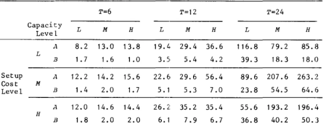
In general, the tree size and the computing time may increase with the planning horizon T. However, since the cost function is more tightly approxi-mated to at the low levels of setup cost and capacity, it can be expected that at each corresponding low level many subproblems might be eliminated by the bound test. This intuition is reflected by the computational results in Table 1 and Table 2. In Table 1, the number of examined subproblems increases with the planning horizon T and the level of capacity, while the level of setup cost does not seem to affect the tree size as significantly as the planning horizon T and the level of capacity.

Table 1. Number of Examined Subproblems and Computing Times (in Second) Averaged over All Demand Patterns and Replications.

T=6 T=12 T=24 Capacity L M H L M H L M H Leve 1 ,~ _{8.2 13.0 13.8 19.4 29.4 36.6 116.8 79.2 85.8} L B _{1.7 1.6 1.0} 3.S 5.4 4.2 39.3 18.3 18.0 Setup i~ 12.2 14.2 15.6 22.6 29.6 56.4 89.6 207.6 263.2 Cost M Level B 1.4 2.0 1.7 5.1 5.3 7.0 23.8 54.5 64.6 A 12.0 14.6 14.4 26.2 35.2 35.4 55.6 193.2 196.

,+

H B 1.8 2.0 2.0 6.1 7.9 6.7 36.8 40.2 50.3

L low, M

=

medium, H

=

high, A number of examined subproblems,

B computing time in second.

Table 2. Percentage of Subproblems Eliminated by the Bound Test and Number of Levels Up from Bottom of Tree at Elimination Averaged over All Demand Patterns and Replications.

T=6 T=12 T=24 Capacity L M H

'"

M H L M H Level A 55.2 45.0 42.9 49.1 45.0 45.5 50.4 47.8 48.8 L B 3.7 3.3 2.9 7.2 6.1 5.2 13.3 11.4 13.2 Seutp _{A 46.5 38.9 37.8 48.6 45.6 44.3 49.6 49.0 48.2} Cost M Level B 3.2 2.9 2.9 6.7 5.9 5.5 12.8 11.7 10.4 A 47.0 39.5 39.7 47.7 44.2 44.8 51.3 48.4 48.9 H B 3.1 2.8 2.8 6.3 5.4 5.4 14.4 11.0 11.6

548 c.S.SungandY.LLee

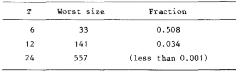
Table 3. The Fraction of the Worst Tree Size to 2T+1.

T 6 12 24 Worst size 33 141 557 Fraction 0.508 0.034 (less than 0.001)

Even if the tree size increases with the planning horizon, Table 3 shows that the fraction of the worst tree size to the maximum possible size 2T+1 for each

T decreases rapidly as T increases.

The number of fathomed nodes by the completeness test is very few. For example, the maximum number fathomed among all examined problems is 8. How-ever, more than 40% of examined nodes are eliminated by the bound test as summarized in Table 2. This implies that the algorithm eliminates about half the examined nodes until it finds a solution. Computational results in Table 2 show that the average depth level of elimination is about half the planning horizon.

In summary, this eV<lluation shows that the algorithm performs weakly as the planning horizon and the levels of setup cost <lnd capacity incre<lse. However, the ratio of tree size to its m<lximum possible size decreases rapidly as the planning horizon incre<lses. And the fathoming test gives rise to eliminate many subproblems at around half the level of the tree throughout all cases. The computing time takes less than 10 seconds for the planning horizons T = 6, 12.

6. Conclusion

A stochastic production planning problem with a finite planning horizon. where cumulative demands up to each period are random variables. is analyzed

based on the solution characteristics of its equivalent deterministic problem. A branch-and-bound algorithm is proposed. which employs a cost approximation procedure of the objective cost function to the convex function at each branching stage. A convex programming algorithm is then incorporated in the branch-and-bound algorithm for lower bound calculations at each subproblem. The performance evaluation experiment concludes that the algorithm may work practically for reasonably sized problems.

paper can include stochastic programming problems with simple recourse, since the associated recourse program part can be expressed in a deterministic program so that an equivalent deterministic program (to the whole program) composed of two deterministic programs can be derived in the similar form of this paper. Further applications may include stochastic transportation-loca-tion problems, and capacity expansion problems with random demands.

As a further research, the authors have been considering a decomposition approach of non linear programming as another treatment of the concave part

(fixed charge) of the cost function.

References

[1] Baker, K.R., Dixon, P., Magazine, M.J., and Silver, E.A.: An Algorithm for the Dynamic Lot-Size Problem with Time-Varying Production Capacity Constraints. Management Science, Vol.24 (1978), 1710-1720.

[2] Bazaraa, M.S. and Shetty, C.M.: Nonlinear Programming. John Wiley & Sons, New York, 1979.

[3] Bitran, G.R. and Yanasse, H.H.: Deterministic Approximations to Stochas-tic Production Problems. Operations Research, Vol.32 (1984), 999-1018. [4] Erenguc, S.S. and Tufekci, S.: A Branch and Bound Algorithm for a

Single-Item Multi-Source Dynamic Lot Sizing Problem with Capacity Constraints. IIE Transactions, Vol.19 (1987), 73-80.

[5] Falk, J.E. and Hoffman, K.R.: A Successive Underestimation Method for Concave Minimization Problems. Mathematics of Operations Research, Vol.l

(1976), 251-259.

[6] Hadley, G.: Nonlinear and Dynamic Programming. Addison-Wesley Publishing Co., Massachusetts, 1970.

[7] Hax, A.C. and Candea, D.: Production and Inventory Management. Pretice-Hall Inc., Englewood-Cliffs, New Jersey, 1984.

[8] Heyman, D.P. and Sobel, M.J.: Stochastic Models in Operations Research, Volume TI: Stochastic Optimization. McGraw-Hill Book Co., New York,

1984.

[9] Nevison, C. and Burstein, M.: The Dynamic Lot-Size Model with Stochastic Lead Times. Management Science, Vol.30 (1984), 100-109.

[10] Press, W.H., Brian, P.F., Teukolsky, P.A., and Vetterling, W.T.: Numeri-cal Recipes, The Art of Scientific Computing. Cambridge University Press, 1986.

[11] Soland, R.M: Optimal Facility Location with Concave Costs. Operations Research, Vo1.22 (1974), 373-382.

550 CS. Sung and Y. J. Lee

[12] Ziemba, W.T.: Stochastic Programs with Simple Recourse, in Mathematical Programming in Theory and Practice. Hammer, P.L. and Zoutendijk, G.

(eds.) North-Holland Publishing Co., 1974.

Chang Sup SUNG: Department of Industrial Engineering, KAIST, P.O. Box 150, Cheongryang, Seoul 131, Korea