RECENT DEVELOPMENTS IN MAXIMUM FLOW ALGORITHMS

Vol. 43, No. 1, March 2000

RECENT DEVELOPMENTS IN MAXIMUM FLOW ALGORITHMS

Takao Asano Yasuhito Asano

Chuo University T h e University of Tokyo

(Received January 7, 1999; Revised September 1, 1999)

Abstract Goldberg and Rao recently proposed the blocking flow method based on a binary length function to obtain a better algorithm for the maximum flow problem. The previous algorithms based on the blocking flow method proposed by Dinic use the unit length function: every residual edge is of length 1. In this paper, we survey properties of the distance function defined by a length function and give an overview on the representative maximum flow algorithms proposed so far in a systematic way by utilizing these properties. Among them are included two new algorithms: the Goldberg-Rao algorithm which finds a maximum flow on an integral capacity network N of n vertices and m edges in ~ ( m i n { m l / ~ , n2/3}7n log(n2/m) log U) time, where U is the maximum edge capacity of N , and the Karger-Levine algorithm which finds a maximum

flow on an undirected network N with unit capacity and no parallel edges in 0 ( m

+

nv3/2) time, where v is the value of a maximum flow of N .

1. Introduction

The maximum flow problem, finding a flow of maximum value on a network from a source to a sink, is one of the most fundamental problems with a wide variety of scientific and engineering applications and has been studied intensively. The problem was formulated by Dantzig [l41 and solved by Ford-Fulkerson [l91 based on the augmenting path method. Since then, a number of algorithms have been proposed and representative algorithms are listed in Table 1. Nice survey papers and books on this topic have also been published 146, 13, 25, 1, 2, 31, 29,6]. The algorithm of Ford-Fulkerson [l91 assumes that input networks have integral or rational capacities and sometimes fails to correctly find a maximum flow or to halt for a network with irrational capacities. Sunaga-Iri [45] proposed a method to find a maximum flow and terminate even for a network with irrational capacities. Dinic [l51 and Edmonds-Karp [l71 independently showed that the Ford-Fulkerson algorithm runs in polynomial time (even for networks with irrational capacities) if flows are augmented along shortest augmenting paths. More specifically, Dinic introduced a shortest augmenting path network, called a level network here, and proposed a blocking flow algorithm to find a maximum flow on a network with n vertices and m edges in 0 ( m n 2 ) time. Karzanov 1371 improved this bound to 0 ( n 3 ) by introducing the concept of a preflow and obtaining a blocking flow in a level network in 0 ( n 2 ) time. Sleator-Tarjan 1441 proposed a dynamic tree data structure, a new data structure suitable for manipulating flows in the level network, and obtained an algorithm for finding a blocking flow in the level network in O(m1ogn) time. This lead to an O(mn1ogn) time algorithm which is considered to be a most efficient algorithm based on the level network.

On the other hand, Goldberg-Tarjan 1261 proposed a new algorithm which was not based on the level network. Their algorithm was called the push-relabel method and uses a preflow introduced by Karzanov and a distance label for each vertex that is a lower bound on the

Maximum Flo W Algorithms 3

Table 1: Representative maximum flow algorithms f23). Years are based on the original

publications while citations are based on the most complete publications.

length of a shortest path to the sink. They obtained 0 ( n 3 ) and O ( m n l o g ( ~ ~ / m ) } time algorithms based on queues and dynamic trees respectively. The push-relabel method had a number of flexibilities and many variants have been proposed. Cheriyan-Hagerup [g]

proposed a randomized algorithm based on a combinatorial game. Their algorithm always finds a maximum flow in O(mn +n2(log n)2) time with probability at least 1 - 2 f i and in O(mn log n) time in the worst case. Alon [S] proposed a derandomization of the Cheriyan- Hagerup algorithm and obtained an

0

(mn

+

TO^ log n) time algorithm. King-Rao-Tarj an

381 also considered a slightly different combinatorial game and obtained an O(mn

+

n2^}

time algorithm for any positive constant e. After that, Phillips-Westbrook [42] obtained an O(mnlogm/n n

+

d ( l ~ g n ) ~ ' ^ ) time algorithm and King-Rao-Tarjan [39] obtained an 0 ( lW4{n iog n ) R) time algorithm (this assumes m

>

n log n and if m

<

TO log n then the time complexity of this algorithm becomes O(mn^g(n2/m))). This slightly improved the Phillips-Westbrook algorithm (for m = n log

n

log log n, the King-Rao-Tarjan algorithm runs a factor of O((1og n)^) faster than the Phillips-Westbrook algorithm).

The shortest augmenting path method, the blocking flow method on the level network, and the push-relabel method described above used a concept of distance based on the unit length function: the length of an edge in a residual network was defined to be one. Goldberg- Rao [23] used a binary length function and obtained an efficient algorithm for networks with

integral capacities. In practical applications, capacities of a network are often represented by approximate integers or rational numbers. Thus, integral capacity constraints make al- most no restriction on practical problems. For the maximum flow problem on networks with integral capacities, we assume that the maximum edge capacity of a network is de- noted by U and every edge capacity is an integer in the range [U,

U\

= {U, l, .

..,

U}.

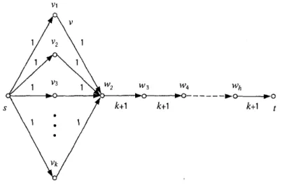
To compare with polynomial and strongly polynomial time algorithms, the similarity assump-

Figure 1: Example of a network N with total path length fl(mn), where edges are directed from left t o right, cap(e) is shown near edge e (cap(e) = 1 is omitted) and a = n and b = n2.

tion log U = O(1ogn) introduced by Gabow [20] is often used. The ballpark bound denoted by 0 " under the similarity assumption is also used (O*(f (n)) = ~ ( ( l o ~ n ) ~ * l ) f (n))). The bound fl(mn) is a natural barrier for maximum flow algorithms and all algorithms de- scribed above are dominated by this bound. In a path decomposition of a flow, the total path length is Q(mn) in the worst case (Figure 1). This implies an Cl(mn) lower bound on any algorithm which augments a flow along an augmenting path. This lower bound does not apply to algorithms that work preflows or use data structures like dynamic trees. In spite of numerous attempts, however, no algorithm described above achieves this lower bound in general. For dense graphs, Cheriyan-Hagerup-Mehlhorn [g] achieved the bound O(n3/ log n) beating the lower bound Wmn). On the other hand, Goldberg-Rao [23] proposed in 1997 an 0(min\m112, n2I3}m log(n2/m) log U) time algorithm beating drastically this lower bound under the assumption of similarity.

For networks with unit edge capacity, the total path decomposition length is 0 ( m ) and o(mn) bounds have been obtained by Karzanov [36] and Even-Tarjan [18], independently. Actually, Even-Tarjan have shown that the Dinic algorithm runs in ~ ( m i n { m ' ^ ~ , n2I3}m) time on networks with unit capacity and no parallel edges. The Goldberg-Rao algorithm [23] achieves this bound (the ballpark bound) for general networks. On the other hand, Goldberg-Rao [24] obtained an O(min{m, n312}m1^2) time algorithm on undirected networks with unit capacities and no parallel edges. Karger-Levine (351 proposed an O ( m

+

nv3l2) time algorithm, where v is the value of a maximum flow on an undirected network with unit capacity and no parallel edges. They also proposed an algorithm with Ofnm2/3u1^) time and a randomized algorithm with O*(m

+

n11/9v) time. The latter algorithm suggests that the maximum flow problem of undirected networks with unit capacity seems easier than the maximum bipartite matching problem, since an O(n2.5) time algorithm [28] has long been fastest for the ipartite matching problem in spite of many efforts for nearly thirty years.

This survey paper is organized as follows. We first give an overview of representative methods in maximum flow algorithms including the shortest augmenting path method, the blocking flow method on the level networks and the push-relabel method in Section 2. We also give fundamental properties of distance labelings defined by length functions and review the Dinic, Even-Tarjan, and Goldberg-Tarjan algorithms in a systematic way based on the distance labeling. Then in Section 3, we consider algorithms for integral capacity networks where scaling of edge capacities is widely used. We see how scaling techniques have been

Maximum Flo W Algorithms 5

used in polynomial time algorithms. The central part of this survey is a description of the Goldberg-Rao algorithm where we try to give several comments on their original algorithm and present a n illustrative example. In Section 4, we consider algorithms for undirected unit capacity networks. Sparsification of a network proposed by Nagamochi-Ibaraki [41] is a most powerful tool in the algorithms recently proposed by Goldberg-Rao [24] and Karger- Levine [35]. We give a brief overview of these two algorithms based on the sparsification and the properties of the distance labelings. In Section 5 we give concluding remarks.

2. Not at ion and Fundamental Algorithms

A

directed graph G = (V, E) having a nonnegative real-valued capacity cap(e) on each edge e E E and two distinct distinguished vertices, a source s and a sink t, is called a network and denoted by N =

(G,

cap, S, t). Throughout this paper, n = IVI and rn =

\E\.

We also use U to denote the maximum edge capacity if all edges have integral capacities. Let &^(v) = {e = (v, W ) E E} denote the set of edges in E out of v. Similarly, & ( v ) = {e = ( U , v) E E} denotes the set of edges in E into v. A flow f on a network N = (G, cap, S, t )

is a real-valued function f on edge set E satisfying the following constraints:

0

<

f (e)

<

cap(e) for all e E E (capacity constraint); _(2.1)

\^

f (e) =

\^

f ( e ) for all v E V - {S, t} (conservation constraint). eeS+ (v) ee6- (v)

(2.2) The value of a flow f , denoted by val(f\ is the net flow out of source S:

By conservation constraint, val(f) is equal to the net flow into sink t. A maximum flow is a flow of maximum value. The maximum flow problem is the problem of finding a maximum flow on a given network. We can assume that all edge capacities are finite, since if some edge capacities are infinite but no path consisting of infinite-capacity edges from S to t exists, then each infinite capacity can be replaced by the sum of the finite capacities without affecting the problem.

For a subset X of V with S E X and t E V - X , let ^ ( X ) be the set of edges out of X (to V - X ) . Similarly, &-(X) is the set of edges out of V - X (to X ) . &+(X)

is called an S-t cut and its capacity is defined by cap(X) = x e e s + ( x ) cap(e). Note that

x e e a + i x ) f (e) -

xee6-

( x i f (e) = val ( f ) and the following famous maximum flow minimum cut theorem holds.

Theorem 2.1 For any flow f and any S-t cut

^(X)

of a network N =

(G,

cap, S, t), an

inequality val(f)

<

cap(X) holds. Furthermore, for a maximum flow f * and an S-t cut S^ (X*) of minimum capacity, val (f

*)

= cap(X*) holds.

2.1. Residual networks and augmenting paths

The Ford-Fulkerson algorithm uses a residual network. For an edge e = (v, W ) E E, let eR = ( W , v) be an edge reversing the direction of e. If e = (v, W ) E E and ( W , v) E, then

we add the edge eR = (W, v) with cap(eR) = 0 . If edges e = (v, W) and e' = (w,v) are both in E then we consider eR = e' and e = em (cap(eR) = cap(el) and cap(etR) = cap(e)) .

Thus, for simplicity, we assume throughout this paper that G is simple and symmetric (i.e., (v, W ) E E if and only if ( W , v) 6 E). This implies E = E U ER

(ER

{eR

1

e 6 E}). For a

Then capf{e) is called a residual capacity of e = ( U , W ) , since we can increase f (e) by

cap(e) - f (e) along e = ( U , W ) and decrease f (eR) along eR = ( W , v) (and thus we can increase flow from v t o W by capf (e) in total). The residual network N ( f ) =

(G( f )

=

[V,

E(f)), capf, S, t) with respect to f is defined to be

Furthermore, if f (e)

>

0 and f ( e R )

>

0 for some e ?

E,

then we can easily modify f without changing the flow value ual(f) and the residual capacities as follows:

Thus, for simplicity, we assume t h a t , whenever f ( e ) is modified, we always perform (2.5) for e, eR E E immediately after t h a t and, thus, a flow f satisfies the following constraint throughout the paper:

f ( e ) = 0 or f ( e R ) = 0 for all e E E. _(2.6) Note that Elf) = E - {e 6 E

\

capf(e) = O} and if cap(e) = f ( e )

>

0 then capj(e) = 0 since f (eR) = 0 by (2.6). A path P = P(s, t) in the residual network N ( f ) from s to

t

is called an augmenting path with respect to f . Actually, define the residual path capacity of P = P ( s , t ) , denoted by A ( P ) , t o be the minimum value among the residual capacities of edges in P (thus A ( P )

>

0) and set

Here, by f ' := f

+

A ( P ) , we mean that we first set

and then perform (2.5) for each e E P (by substituting f 1 for f ) . Thus, the obtained f 1 satisfies flow constraints and (2.6) and f ' is a flow on N with ual( f') = ual( f )

+

A ( P )

>

val(f

).

Note that, before performing (2.5), some f l ( e ) may be larger than cap(e), and t h a t , after performing (2.5), some f ' ( e f ) with e' E P may be zero. We have, however, capf~ (e) = cap (e) - A ( P ) and caprt (eR) = capf{eR)

+/\{P)

for each e E P unless P contains both e and eR, since the residual capacity of edge e E P is not changed by performing (2.5). (If P contains both e and eR, then capp (e) = capf(e) and capp (eR) = capf (eR)

.)

Thus, we can increase the value of a flow by sending a flow along an augmenting path. This implies t h a t , if f is a maximum flow on N then there is no augmenting path with respect to f . The converse is also true and the following theorem holds.

eorem 2.2 For any flow f on N = (G, cap, s , t ) , f is a maximum flow if and only if there is no augmenting path with respect to f .

Proof. Since the necessity is already described above, we consider the sufficiency. Suppose t h a t there is no path from s t o t in the residual network N ( f ) . Let X be the vertex set reachable from s in N ( f ) . Then s E X and t E V - X and @ ( X ) is an S-t cut of N .

By the definitions of X and N ( f ) , each edge e E (X) of N satisfies f (e) = cap(e), f (eR) = 0 (capf (e) = 0) and each edge e E 6 - ( X ) of N satisfies f (e) = 0, f (eR) = cap(eR) (capf (eR) = 0). Thus,

Maximum Flo W Algorithms 7

Since, for any flow f and any s-t cut 6J^{X1) of N , an inequality ual(fl)

<.

cap(X1) holds, we have ual( f ) = cap(X) >_ ual( f l) and cap(X) = ual( f )

<

cap(X1). Thus, f is a maximum

flow and (X) is an s-t cut of minimum capacity in N. 0

Based on the above observation, Ford-Fulkerson obtained the following algorithm.

Ford-Fulkerson Algorithm

1. Set f := 0 (i.e., f (e) := 0 for each edge e E E).

2. Repeat finding an augmenting path' Pf with respect to f and augmenting the flow by f := f

+

A ( P f ) until there is no augmenting path Pf with respect to f .

If all edge capacities are integers, then one can easily obtain by induction that, at any time of the iterations, the edge capacities of N ( f ) and A ( P f ) are integers and a flow f is integral (i.e., f (e) is an integer for each e E E). Thus, we have the integrality theorem as follows.

Theorem 2.3 -If all edge capacities are integers, then there is a maximum flow f such that f (e) is an integer for every e ?

E.

Since any flow f " on the residual network N ( f ) can be decomposed into a set of paths

P

with fl'(e) = A ( P ) , we can use the notation

extending (2.7) t o augment f to f ' using /l1. Furthermore, if fl' is a maximum flow on N ( f

),

then f := f

+

f " is a maximum flow of N . Such a maximum flow fl' is called a maximum residual flow of f .

2.2. Blocking flows and level networks

As mentioned in Introduction, the Ford-Fulkerson algorithm may have many augmentations if the network has large integral capacities and it sometimes fails to correctly find a maximum flow or to halt if the network has irrational capacities. Thus, we have to select augmenting paths carefully so that their method becomes efficient. Dinic and Edmonds-Karp indepen- dently showed that the Ford-Fulkerson algorithm runs in polynomial time (even for networks with irrational capacities) if augmentations are done along shortest augmenting paths. In this section, we give an overview of the Dinic algorithm.

Figure 2: A blocking flow f " of value 1 on a level network NL

( f )

(f "{e)/capf (e)) Dinic used a blocking flow and a level network (Figure 2). A flow fl' is a blocking flow of the residual network N ( f ) = (G(/) = (V, E ( f ) ) , c a p f , s , t ) with respect to a flow f on N =

(G,

cap, S, t ) if any path from S to t has an edge e with fl'(e) = capf (e)

>

0, that is, there is no path from s t o t in the network obtained from N ( f ) by deleting all edges e with

f"(e) = capf (e)

>

0.

A

level network N d f ) = (Gi(f) = (V, EL(

f ) ) ,

cap,, S, t) of N ( f ) is the network obtained from N ( f ) by choosing all the edges in shortest paths in N ( f ) from s to t (a shortest path from s to t here is a path from s to

t

containing the minimum number of edges) and

EL(f)

C

{(u,v) G E(f)

1

levei[u] = level[v]

+

l}

where level[v] is the length (i.e., the number of edges) of a shortest path in N ( f ) from a vertex v to t. The levels level [v] of all vertices U can be computed in 0 ( m ) time by the breadth-first search for N ( f ) . Now the Dinic algorithm can be written as follows.

Dinic Algorithm

1. Set f := 0 (i.e., f (e) := 0 for each edge e E E).

2. Repeat finding a blocking flow f " on the level network NL( f ) of the residual network N ( f ) and augmenting f := f + f " until there is no path from s to t in N ( f ) .

Let l e v e l ~ s } denote level[s] in the k-th iteration of finding a blocking flow. Then it can be shown that l e ~ e l ~ + ~ [ s ]

>

levelk[s] holds due to blocking flows (see Lemma 2.7 later). Thus there are a t most n - 1 iterations. In each iteration, a blocking flow can be computed in 0 ( m n ) time by the depth-first search for the level network NL(f). Thus, the following theorem is obtained.

Theorem 2.4 The Dime algorithm finds a maximum flow f on N in 0 ( m n 2 ) time.

2.3. Length functions and distance labelings

Let N (

f )

= (G( f

),

capf, S, t ) be the residual network with respect to f . A length function

C.

is a function on E ( f ) t o nonnegative numbers. For a labeling function d on V with d(t) = 0 and a length function

l

on E( f ) , a reduced length of edge e = ( U , U ) E E ( f ) is defined by

&(e) = C.(e)

+

d(v) - d(u). The labeling function d is called a distance labeling if the reduced lengths of all edges are nonnegative. Such a distance labeling always exists here since there is no negative cycle in N (

f )

with respect to the length function C.. Let d,Av} be the length of a shortest path from v to t in N ( f ) with the length function C.. Then ds. is a distance labeling and the following inequality holds for any distance labeling d of N ( f ) :

d

<:

ds. (i.e., d(v)

<

dl(v) for any v ? V).

Thus, dt can be called the maximum distance labeling. Note that, by the linear programming duality, the shortest path problem can be formulated as the dual problem for the problem of maximizing d with the constraint that d is a distance labeling.

For a flow f and a length function C. of N ( f ) , an edge e = (U, v) G E( f ) satisfying de(u) = de(v)

+

C.(e) is called admissible in N ( f ) and the shortest residual network Nl(f) is the network obtained from N ( f ) by deleting the edges not contained in any shortest path from s to

t.

That is, the edge set E;( f ) of N f ( f ) is a subset of admissible edges of N ( f ) and defined as follows.

El(f) = {e

c

E ( f )

1

e is contained in ashortest path from s t o t in N ( f ) } Of course, the capacity of e G E&) = El(f) E(/) is kept the same.

Let P be a path in N^f) from s to t and 0

<

A'

5

A ( P ) ( A ( P ) is the residual path capacity of P). We try to augment the current flow f by pushing a flow of value A' along P and obtain a flow f

'

:= f

+

A' (by extending (2.7), f

'

:= f

+

A' means that we first set

f

(e)

+

A' (e E P)

Maximum Flo W Algorithms 9

and then perform (2.5) for each e E

P

(by substituting f' for f

)).

We also update the length function l to l using a nonnegative function

P'

as follows:

Note that it is possible that capf- (a )

#

capf ( a ) in spite of / ' ( a ) =

f

( a ) since c a p f / ( a ) =

cap(a) - f ' ( a )

+

f

' ( a R ) and cap ( a ) = cap(a) -

f

( a )

+

f

( a R ) . If capf- (a ) = 0

<

capf ( a ) ,

then a is not in

N ( f l )

and we assume that £"(a = oo holds implicitly. Then we have the following lemma.

Lemma 2.5 dp is a distance labeling of N ( f l ) with respect to '?t defined by (2.10).

Proof. The lengths are changed according to the residual capacities and the residual

capacities are changed only for the edges a and aR with a in

P.

Therefore, it suffices to show that de satisfies the requirement of a distance labeling with respect to ¥C only for such edges.

If capf- (a )

<

capi(a) for an edge a = ( U , v ) , then a 6 P n E p ( f ) and we have dt(v)+l1(a)

>

d d v )

+

i(d)

= dp(u) by I 1 ( a ) - l ( a ) = P ( a )

>

0. If capf- (a )

>

capf ( a ) for an edge

a = ( u , v ) , then aR = ( v , u ) E

P

n

E p ( f ) and d ( ( v ) = l ( a R )

+

dp(u)

>

dp(u), and thus

d d v )

+

('{a)

>,

& ( v )

>

d t ( u ) . U

Note that P can contain a cycle of length 0 although it does not go through the same edge twice or more. Thus, P may not be simple. By Lemma 2.5, the maximum distance labeling d y with respect l satisfies din

>

dp. We can generalize Lemma 2.5 as follows. If f "

is a flow on the residual shortest network Np ( f ) of N ( f ) , then f " can be decomposed into a

set of flows along shortest paths in Np( f ) . Considering each such a flow in the decomposition independently and simultaneously, we have the following corollary.

Corollary 2.6 If f" is a flow on the residual shortest network N p ( f ) of N ( f ) , then, for f := f

+

f " , dn is a distance labeling of N ( f l ) with respect to

C1

defined i n (2.10) and thus dP

>

dp.

Note that, in the Dinic algorithm, each edge in N ( f ) has unit length and the level network exactly corresponds t o the residual shortest network. The levelk[s] in the k-th iteration can be shown t o satisfy l e ~ e l ~ + ~ [ s ]

>

levelk[s] as a special case of the following lemma.

Lemma 2.7 If fl' is a blocking flow on the residual shortest network N p ( f ) of N ( f ) and all

edges lengths i n

t

of N ( f ) and i n

I"

of N ( f

')

with f

'

:= f

+

f" are positive, then d f { s )

>

dp(s) (l' is defined i n (2.10)).

Proof. Let ~ : ( f ) be the network obtained from N p ( f ) by adding all edges eR with length 0 for edges e in Np( f ) . Note that dp(u) = dAv} + l ( e )

>

d&) for an edge e = ( U , v ) of Np(

f )

and thus eR = ( v , U ) is a kind of backward edge directed from a vertex of less distance to a vertex of larger distance in N p ( f ) and thus eR is not in N p f f ) . Furthermore, if eR = ( v , U ) is of length more than dp(v) - dp(u) ( d i ( v ) - d { ( u )

<

O), then its addition to Ni( f ) makes

no effect on the shortest paths in

NAf)

from s to t.

Let N F ( ~ ) ( N ? ( f ) , resp.) be the network obtained from Np( f ) ( N : ( f ) , resp.) by deleting all edges a with capf ( a ) = f " ( a ) . Then there is no path in Ni( f ) (and in

Nf{

f )

of length a t most dp(s)) from s to

t ,

since f" is a blocking flow of Np( f ) . Let N W be the network obtained from N: ( f ) by adding all edges e in N ( f ) but not in N: ( f ) . Then, any path from s to

t

in the network N * ( f ) is of length greater than d f { s ) , since all edges a with

Figure 3: For threshold a, only edge ( U , v) is of length 0 and all other edges are of length 1. Thus, dl(s) = 2. If we augment the current flow by using a blocking flow along a shortest path S, U, v, t of length 2 and increase the flow value by 1, then, in the residual network in the next time, the edge (v, U) satisfies P(v, U ) = 0 and thus dp (S) = 2.

Note t h a t the edge set of N ( f l ) is a subset of the edge set of N h ( f ) and the length £

is a t least the length of N k ( f ) and thus, any path from s t o t in the network N ( f l ) is of length greater than de(s).

By this lemma, we can estimate the number of iterations of finding a blocking flow in a maximum flow algorithm. If we use the unit length function C, of N ( f ) as in the Dinic algorithm, then the level network NL (f

)

of N (f ) exactly corresponds t o the residual shortest network Ng( f ) of N ( f ) and the number of iterations is O ( n ) . Goldberg-Rao introduced a concept of volume which can also be used t o estimate the number of iterations. Consider an edge e in N ( f ) as a pipe and the residual capacity capf (e) of e as an area of the cross section of pipe e. Then capf[e)£(e becomes the volume of pipe e and the total volume Volfe of the residual network N ( f ) is

The difference of the value of a maximum flow f * and that of a current flow f , denoted by val(f

*)

- val( f}, can be estimated as follows by using this volume, since if we augment f by a flow of value 1 along an augmenting path in N ( f ) from S to t then the volume decreases

by a t least dt(s) (note that VolM is nonnegative by the definition).

Lemma 2.8 [23] For a maximum flow f * and a current flow f on N and a length function

By Lemmas 2.7 and 2.8, to decrease the number of iterations, the number of different values which dl(s) can take on and the value Volft should be made small. This leads us t o the following strategy: edges with large residual capacity should be of shorter length. More specifically, all edges with large residual capacities should be of length 0. However, if we allow a general length function, then analysis becomes harder. From these kinds of viewpoints, a binary length function  with £(a = 0 or £(a = 1 for each a may be of help. Goldberg-Rao [23] considered a binary length function

i

such t h a t £(a = 0 if capf(a) >_ a and £(a = 1 if 0

<

capf(a)

<

a for some threshold a. However, the existence of edges of length 0 makes Lemma 2.7 violated in some cases (Figure 3). In spite of these weak points, a binary length function C, has nice aspects described below.

Using a maximum distance labeling de, let Sk = {v E V

1

d M

>

k} (k = 1 , 2 , . .

.,

dl(s)) and define < ^ ( S ) S-t cuts

^{Sk}

of N ( f ) t o be canonical cuts of N ( f ) . Canonical cuts

Maxim um Flo W Algorithms 11

can be rewritten by S+(Sl,} = E(Vk, Vf-l) if we use Vk

=

{v E V

\

di(v) = k} and E(Vk,Vk.l) {a = ( u , v ) E E(/)

1

dt(u) =

k,

di(v) = k - l}. Let

S

be a set in

5

= {Sl, Ss, . . .

,

Sd,

such that capj

(S)

= mmsi, {cap (Sk)}. That is, &+ ( S ) is a canonical cut of minimum capacity. Then the value val( f 'I) = val( f

*)

- val( f ) of a maximum residual flow f " on N ( f ) (f * := f

+

f") can be bounded by capf(S) and the following lemma is obtained.

Lemma 2.9 [23] Let

i

be any binary length function of N ( f ) and S+(S) be a canonical cut of N (

f )

of minimum capacity. Then

where fl' is a maximum residual flow on N ( f ) (f * := f +

f")

and

fi

is the maximum residual capacity of edges of N ( f ) of length 1.

Proof. Consider V&+l U V& (k = 0,1,

...,

[%!$l

- 1). If all such sets had more than

&

vertices, then the network N would have more than n vertices and a contradiction is obtained. Thus, there is a set V'&+l UVat with a t most

Ñ

vertices. Then we have cap

f(S)

<:

2 2

f i \ E ( h k + l ,

Va}\

5

/3

(&)

since N is simple and lE(hk+l,

Va)\

<

lhk+l

l

l h k

l

(&)

_-

D

By Lemmas 2.7, 2.8 and 2.9, we have the following lemma and theorem for unit capacity networks.

Lemma 2.10 For a flow f in a unit capacity network N , let Er be the set of edges a with f (a) = 1. Then there is a flow f of value r such that \Ef

\ <:

2nfi.

Proof. Using the Ford-Fulkerson algorithm, we initially set

f'

:= 0 and repeat augmenting f along a shortest path in N ( f l ) from s to

t

(with the unit length function C) and increase the flow value by 1 until the value of flow f

'

becomes r . Let f be the flow f ' of value r

obtained in this way. We rewrite N to be the unit capacity network with edge set Ef

.

Then N contains no directed cycle since we used shortest augmenting paths. Now try again t o find the flow f of value r in N by the same method as above. Then, for a flow f of value r' in (r'

+

l)-st iteration, f - f

'

is a maximum residual flow in the residual network N ( f

')

and dl ( S ) satisfies dl ( S )

<

-7Ñ

by Lemma 2.9 and

fi

= 1. Thus, in (r'

+

l)-st iteration, the flow value is increased from r' to r'

+

l and a t most

&

edges are newly used to augment flow f l . This implies

Theorem 2.11 [36, 181 The Dinic algorithm finds a maximum flow on a unit capacity network N with no parallel edge in 0(min{m1I2, n2I3}m) time.

Proof. Since the residual capacities are 1 or 2 in the residual network and each blocking flow can be obtained in 0 ( m ) time, we can assume that there are a t least min{m112, n2I3} iterations of finding a blocking flow (otherwise the theorem trivially holds). Thus, the maximum flow f * is of value a t least min{m1I2, n2I3} and val(f*)

<:

n

<:

m since N has no parallel edge. We will show below that there are a t most 3 min{m112, n2I3} iterations of finding a blocking flow. Let i be the unit length function.

We first consider the case when m1I2

<

n2I3. After the m^-th blocking flow iteration, the flow f is of value a t least m112 and dl(s)

>

m1I2 by Lemma 2.7. By Lemma 2.8, we have

and there are a t most 2m112 blocking flow iterations after the m^-th blocking flow iteration. Next we consider the case when m112

>

n2I3. After the n2I3-th blocking flow iteration, the flow

f

is of value a t least n2I3 and df(s)

2

n213 by Lemma 2.7. By Lemma 2.9, we have

and there are a t most 2n2^ blocking flow iterations after the n213-th blocking flow iteration.

D

2.4. Preflows and push-relabel method

A preflow f on a network N = (G = (V, E), cap, S, t ) is a real-valued function f on edge set E satisfying the following constraints [37]:

0

<

f (e)

<

cap(e) for all e E E (capacity constraint); (2.11)

f

(e) - f (e)

2

0 for all v E V - { S } (preflow constraint). (2.12) e€ ( v ) e â ‚ ¬ d + (

The value ex(v) E e c < - ( v )

f

(e) - E e g i t + ( v )

f

(

e) is called an excess of v and a vertex U E

V - {S,

t}

is called active if ex(v)

>

0. Clearly ex(s)

<

0 by the preflow constraint. Note t h a t the only difference between flows and preflows is ex(v) = 0 in a flow but ex(u)

>

0 in a preflow for each vertex v E V - {S, t}. Thus, we use the same terms, notation and requirements (except preflow constraint) for preflows as for flow introduced before in this paper. An edge e E E is saturated if capf (e) = 0 and unsaturated otherwise. (The capacity constraint implies t h a t any unsaturated edge e has capf (e)

>

0 and the residual network N( f ) of preflow f consists of the unsaturated edges.)

We describe the Goldberg-Tarjan push-relabel method based on preflows [26] by bor- rowing the summary given by Ahuja-Orlin-Tarjan [4]. The preflow algorithm maintains a preflow f and moves flow from active vertices through edges in N ( f ) toward the sink t, along estimated shortest paths. Excess flow that cannot be moved to the sink t is returned to the source S, also along estimated shortest paths. Eventually the preflow becomes a maximum

flow.

As an estimate of path lengths, the algorithm uses the unit length function k' and a distance labeling d of N ( f ) such t h a t d(s) = n , d(t) = 0 and d(v)

<

d(w)

+

!(e) for every edge e = (U, W ) of N ( f ) We) = 1). (Recall t h a t , for a labeling function d on V with d(t) = 0 and a nonnegative length function .l on E( f ) , if the reduced length &(e) = t(e) +d(w) - d(u) of each edge e = ( U , W ) E E(/) is nonnegative, then d is called a distance labeling.) Let dg(u) be the length of a shortest path from U to t in N ( f ) with length function k' as before. Then

df is the maximum distance labeling and the requirement for d t o be a distance labeling implies there is no path in N ( f ) from s to t since d

5

dl holds (i.e., d(u)

5

dt(u) for any U E V). Furthermore, a proof by induction shows that, for any distance labeling d in the algorithm, d(u)

<

min{dl(u, S)

+

n , df (v, t)}, where de(u, W ) is the length of a shortest path from v t o W in N ( f ) . An edge e = ( U , W ) of N ( f ) is called eligible if d(u) = d(w)

+

1. Note

Maxim um Flo W Algorithms 13

that df,(v) = dl(v, t) and that the term eligible is defined by using a distance labeling d while the term admissible was defined by using the maximum distance labeling dt.

More specifically, the algorithm initially sets

f (e) :=

{

~ ( e ) if e E & + ( S ) ,

if e E

E

- & + ( S ) , d (v) := min{dl(v, S)

+

n, dt (v, t)}.

Thus, initially, f is a preflow and d is a distance labeling. Note that d(s) = n and d(t) = 0 since there is no edge in N

( f )

out of s and dl(s, t ) = oo. The algorithm consists of repeating the following two steps which maintain a preflow f and distance labeling d, in any order, until no vertex is active:

Push(v, W).

Applicability: Vertex v is active and edge e = (v, W ) is eligible.

Action: Increase f (e) by min{ex(v), capf(e)} (we mean that we first set

f

(e) :=

f

(e)

+

min{ex(v), capf (e)} and then

f ( e ) :=

f

(e) - min{f(e),

f

(eR)};

f

(eR) := f ( e R ) - min{f (e),

f

(eR)}

as before). The push is saturating if e = (v, W ) is saturated after the push and

nonsaturating otherwise. Relabel(v).

Applicability: Vertex v is active and no edge e E E(f) out of v is eligible.

Action: Replace d(v) by min{d(w)

+

1

1

e = (v, W ) E E(f) out of v is unsaturated}.

When the algorithm terminates, f is a maximum flow. Goldberg-Tarjan derived the following bounds on the number of steps required by the algorithm.

Lemma 2.12 [26] Relabeling a vertex v strictly increases d(v) . No vertex label d(v) exceeds 2n - 1, and the total number of relabelings is 0 ( n 2 ) .

Lemma 2.13 [26] There are at most O(mn) saturating pushes and at most O(n2m) non- saturating pushes.

Efficient implementations of the above algorithm require a mechanism for selecting push- ing and relabeling steps to perform. Goldberg-Tarjan proposed the following method: For each vertex, construct a (fixed) list A(v) of the edges out of v. Designate one of these edges, initially the first on the list, as the current edge out of v. To execute the algorithm, repeat the following step until there are no active vertices:

Push/Relabel(v).

Applicability: Vertex v is active.

Action: If the current edge (V, W) of v is eligible, perform push(v, W). Otherwise, if

(v, W ) is not the last edge on A(v)

,

make the next edge after (v, W ) the current one.

Otherwise, perform relabel(v) and make the first edge on A(u) the current one.

With this implementation, the algorithm runs in O(nm) time plus O(1) t ' ime per non- saturating push. This gives an O(n2m) time bound for any order of selecting vertices for push/relabel steps. Making the algorithm faster requires reducing the time spent on non- saturating pushes. The number of such pushes can be reduced by selecting vertices for pushlrelabel steps carefully. Goldberg-Tarjan [26] showed that first-in, first-out selection (first active, first selected) reduces the number of nonsaturating pushes to 0 ( n 3 ) . Cheriyan- Maheshwari [l01 showed that highest label selection (always pushing flow from a vertex with

highest label) reduces the number of nonsaturating pushes to 0 ( n 2 d 2 ) . (The latter rule was first proposed by Goldberg [22], who gave an 0 ( n 3 ) bound.)

Figure 4: Example of a level network TVL(/") whose edges on the path from w2 to

t

are searched many times by the Dinic algorithm.

2.5. Dynamic trees implementations

The Dinic algorithm finds a blocking flow on a level network N L ( f ) by doing the depth-first search from s in N L ( f ) and saturating one edge at a time. But this wastes much time since edges are searched many times as shown in Figure 4. To reduce the time per edge saturation, we should keep track of the flow by using appropriate data structures. Galil- Namaad [21] and Shiloach [43] discovered a method of this kind that runs in 0(m(log n)2) time. Sleator-Tarjan [44] improved the bound to O ( m log n) inventing the data structure of dynamic trees. Goldberg-Tarjan [26] obtained a O(mn log(n2/m)) time algorithm for finding a maximum flow on a network N based on the push-relabel method implemented by using dynamic trees.

3. Maximum Flow Algorithms for Integral Capacity Networks

As described in Theorem 2.11, Karzanov [36] and Even-Tarjan [l81 have shown indepen- dently that the Dinic algorithm runs in 0 ( m i n { d 2 , n2I3}m) time on networks with unit capacities and no parallel edges. For general integral capacity networks, Edmonds-Karp [l71 obtained an O(m210gU) time algorithm and Dinic [l61 and Gabow [20] improved this bound to O(mn\ogU) (note that U is the maximum edge capacity of a network). They used a scaling method. Ahuja-Orlin [3] combined this scaling method with the push- relabel method of Goldberg-Tarjan based on preflows [26] and obtained an 0 ( m n + n 2 log U) time algorithm. Ahuja-Orlin-Tarjan [4] explored possible improvements to Ahuja-Orlin algorithm and obtained an 0 ( m n

+

n2(10g u)lI2) time algorithm and an O(mnlog(2

+

(n/m) (log U) l/')) time algorithm. Goldberg-Rao [23] further improved these bounds and

obtained an 0(min{m1I2, n2I3}m log(n2/m) log U) time algorithm beating drastically the lower bound O(mn) on the path decomposition method under the similarity assumption l o g = Q(1og n ) introduced by Gabow.

In this section, we review the scaling method of Gabow [20] and the Ahuja-Orlin algo- rithm briefly and describe the Goldberg-Rao algorithm extensively.

Maxim urn Flo W Algorithms

3.1. Scaling method

Let N = (G, cap, S, t ) be a given network with integral capacities. Set N o :=

N

and recur- sively define Ni+l = (GG1, s, t ) to be the network obtained from Ni = (Gi, capi, s, t ) by setting capi+' (e) := 1capi(e)/2\ for each edge e in N'

(i

= 0,1, . .

.,

[log U\ - 1). Since every edge is of capacity 0 or 1 in N1l0g '1, a maximum flow f llOgu-! can be obtained in O(mn) time. Assume that a maximum flow f '+l on Ni+l is already obtained and consider the residual network N^(2fi+') of N^ with respect to flow 2fi+'. Note that any path P in Ni(2 /'+l) from S to

t

has the residual path capacity A ( P )

5

1, since otherwise P is a path in Ni+l(f^l) from S to t with residual path capacity A ( P )

>

1 and contradicts that /'+l is a maximum flow on Ni+l. Thus, for a maximum flow g' on Ni(2 f '+l), f := g'

+

2 f '+l is a maximum flow on Ni and val(g1} = val

(f

1}

- val(2 /'+l)

5

m since g' = f i - 2 f i + l can be decomposed into a set of paths in Ni(2 /'+l) each with the residual path capacity 1. This implies that we can find a maximum flow f i on N' by at most m augmentations. Each augmentation can be done by finding a path from S to t in 0 ( m ) time and we can obtain f ^ on Ni in 0 ( m 2 ) time. Thus, a maximum flow in N can be obtained in O(m2 1ogU) time. Gabow [20] improved this bound t o 0 ( m n log U).

3.2. Ahuja-Orlin algorithm

In this section we describe the Ahuja-Orlin scaling algorithm [3] by borrowing the summary

given by Ahuja-Orlin-Tarjan [4]. This enables us to understand the Goldberg-Rao algorithm in the next subsection easily. The intuitive idea behind the Ahuja-Orlin algorithm is to move large amounts of flow when possible. One way to apply this idea to the preflow algorithm is t o always push flow from a vertex of large excess to a vertex of small excess, or to the sink. The effect of this is to reduce the maximum excess a t a rapid rate.

Making this method precise requires specifying when an excess is large and when it is small. For this purpose the Ahuja-Orlin algorithm uses an excess bound A and an integer scaling factor k

>

2. A vertex U is said to have large excess if its excess exceeds A/k and

small excess otherwise. As the algorithm proceeds, k remains fixed, but A periodically decreases. Initially, A is the smallest power of k such that A

>

U. The algorithm maintains the invariant that ex(v) <_ A for every vertex v. This requires changing the pushing step described in Section 2.4 to the following:

Push(u, W).

Applicability: Vertex v is active and edge e = (v, W ) is eligible.

Action: If W

#

t, increase f (e) by min{ex(v), capf(e), A - ex(w)}. Otherwise (W = t )

,

increase f (e) by min{ex (v), cap (e)

}

.

The algorithm consists of a number of scaling phases, during each of which A remains constant. A phase consists of repeating pushlrelabel steps, using the following selection rule, until no active vertex has large excess, and then replacing

A

by A/k. The algorithm terminates when there are no active vertices.

Large excess, smallest label selection: Apply a push/relabel step to an active vertex v of large excess; among such vertices, choose one of smallest label.

Since the edge capacities are integers, the algorithm terminates after at most llogk U\

+

1 phases. After [logi. U\

+

1 phases, A

<

1, which implies that f is a flow, since the algorithm maintains integrality of vertex excesses. Ahuja-Orlin derived a bound of O(kn2 logfl) on the total number of nonsaturating pushes. Choosing k to be a constant independent of n gives a total time bound of O ( n m

+

n2 log U) for this algorithm, given an efficient implementation of vertex selection rule. One way to implement the rule is to maintain an array of sets indexed by vertex label, each set containing all large excess vertices with

corresponding label, and to maintain a pointer to the nonempty set of smallest index. The total time needed to maintain this structure is 0 ( n m

+

n2 log U).

Ahuja-Orlin-Tarjan [4] improved the Ahuja-Orlin algorithm and obtained an 0 ( m n

+

n2 (log U) 'l2) time algorithm and an

0

(mn log(2

+

(n/m) (log

U)

'l2)) time algorithm.

.

Goldberg-Rao algorithm

In this section, we give an overview of the Goldberg-Rao algorithm which drastically cleared the barrier ^(mn) of path decomposition methods under similarity assumption. Its ballpark complexity is 0* (min{m3I2, mn2I3

})

.

Let f * be a maximum flow and let f be a current flow on N. They tried to esti- mate the difference between the maximum flow value and the current flow value val( f

*)

-

val(f) using some upper bound F. Since U is the maximum edge capacity and val(f*)

<^

x(<i,w)eii+(ç cap($, W)

<

n u , they first set F := n u .

In each phase of the Goldberg-Rao algorithm, the updates are repeated until val(f*) -

val(f) is assured to be no more than F/2. Then a next phase starts setting F := F/2. If F

<

1, then a maximum flow is obtained since each capacity is integer and we terminate. Thus the number of phases is a t most 1

+

log(nU).

At the beginning of each phase, we define A to be

and find a flow f " of value A or a blocking flow f " of value a t most A and augment f := f

+

f". In each phase, augmentations using a flow of value A occur at most min{m112, n213} times and augmentations using a blocking flow can also be shown to occur a t most 0(mir{m1I2, n213}) times. Furthermore, such an augmentation using a flow f " of value A or a blocking flow f " of value a t most A can be obtained in 0(mlog(n2/m)) time based on the special structure of the treated network. Thus the time complexity of the Goldberg-Rao algorithm becomes ~ ( m i n { m l / ~ , n2I3}m 1og(n2/m) log(nU)). We can further improve log(nU) in the bound to log U.

The key point in the Goldberg-Rao algorithm is a binary length function  such that ^(a) = 0 if capf(a)

2

a and £(a = l if 0

<

capf (a)

<

a for some threshold a . However, the existence of edges of length 0 makes Lemma 2.7 violated in some cases (Figure 3). To cope

with these situations, they introduced a notion of special edges.

Goldberg-Rao algorit hrn

1. Initialize f := 0, F := n u , and A := f^n$2

,

1

, 7 1 1 ) -

2. (Iterations of phase step) (we choose a = 5A - 4 and a~ = 2A - 1)

(a) If F

<

1 then terminate (f is a maximum flow). Otherwise, go to the following update step.

(b) (Iterations of update step)

i. Compute the residual network N ( f ) and define a length function £(a on a E E ( f ) as follows (Figure 5(a)):

£(a = 0 (capf (a)

2

a ) 1 (0

<

cap (a)

<

a).

ii. Compute the maximum distance label de of N ( f ) for l . If de(s) = 0, then find a flow g of value a~ along a shortest path of N ( f ) from s to

t ,

and go to X (2(b)x). Otherwise, proceed to the following.

.

Maximum Flo W Algorithms 17

Figure

5:

A

residual network N ( f ) with

A

= 3, a = 11 and OIL = 5. (a) Thick edges are of length 0 and the others are of length 1 in l . (b) Thick broken edges are special edges. Thick edges are of length 0 and the others are of length 1 in t.

iii. iv. V. vi. vii. . . . V l l l . ix.

Find a canonical cut S'^'(S) of

N(

f ) of minimum capacity.

F

1

and go t o If cap(S)

5

F/2 then set F := cap(S) and

A

:= fmin~m1/2,n2/31

2 (terminate the update step and go t o the next phase step). Otherwise, proceed t o the following.

Consider a = (U, v) E

E(

f ) satisfying a^

<

capf (a)

<

a, de(u) = ddv) and capf (aR)

>

a t o be a special edge and modify the length function l above t o the following length function (Figure 5(b)):

0 (if e is a special edge) Fie) =

l(e) (otherwise).

(Note t h a t de = dc, i.e., d d v ) = dl(v) for each v E V).

Compute the shortest residual network N,{f) of N ( f ) with respect to (Figure 6(a)). (Note that

Nl(f)

contains no cycle of positive length.)

Compute the network Ns'[ f ) obtained from NE( f ) by contracting each strongly connected component (it consists of only edges of length 0) into a vertex (Figure 6(b)). (Note that N j ( f ) contains no directed cycle.)

Find a flow f It of value A or a blocking flow f " of value a t most A in N j ( f ) . Extend the flow f l' in N; ( f ) t o a flow g in Nl( f ) by extending each contracted vertex U of N'/{ f ) to the corresponding strongly connected component S T ( u )

of NZ(f) (Figure 7(a)) and properly distributing the flow going through v in S T ( u ) as follows if ST(v) has positive or negative excess vertices (for flow f " and escfl~ (U) =

Eee6+(u)

f"(e) -

ze&i-(u)

ft1(e), a vertex U E V - {S,

t }

is

called a positive excess vertex if exftl(u)

>

0 and a negative excess vertex if exf11 (U)

<

0). Choose a vertex rU in ST (v) as

and construct two directed rooted trees I N ( u ) and OUT(v) with the same root ru in ST(v) where I N ( v ) is an intree and OUT(v) is an out tree (Figure

Figure 6: (a) Maximum distance labeling dg of the residual network N ( f ) in Figure 5 with

A

=

3,

a = 11 and =

5.

A,

B,

C

are strongly connected components and edges marked with X are deleted in NE(f). (b) NF(f) obtained from NZ( f ) by contracting the strongly connected components and a flow f " of value

A

in N!( f )

(

f1'(e)/capf (e)).

7(b)) (there is a unique path from each vertex t o r,, in I N ( v ) and there is a unique path from r,, t o each vertex in OUT(v)). Along a path from each positive excess vertex U to r,, in I N (v) we distribute a flow of value exf11 (U)

>

0. Then along a path from r,, to each negative excess vertex U in OUT{v) we distribute a flow of value -ex fii{u)

>

0. The flow g in NZ(/) is obtained in this way (Figure 8).

X. Update the flow

f

to f := f

+

g and go to (b).

This algorithm uses a flow f " of value a t most A in the network N i ( f ) with no positive cycle and satisfies the following

A-

invariant:

for each vertex v , the incoming flow value

Seed-(,,)

fl'(e) and the outgoing flow value

Seed+(,,)

f "(e) are both a t most A.

Thus, fl'(a)

<

A

for each edge a in N / ( f ) . Furthermore, for each strongly connected component S T ( v ) corresponding to a contracted vertex U in N D ) , a flow of value exf11 ( U ) is augmented along a path from each positive excess vertex U t o r,, in I N ( v ) and a flow of value -exj11 ( U ) is augmented along a path from r,, to each negative excess vertex U in OUT(v). Thus, the total flow value through each vertex in I N ( v ) is a t most A - 1 if S T ( v ) does not contain S, t since r,, is positive excess vertex. Similarly, the total flow value

through each vertex in O U T (v) is a t most

A.

This implies t h a t g(a)

5

2A

-

1

for each edge a in a strongly connected component S T ( v ) without S , t for the extended flow g of f". If ru = t then there is no negative excess vertex in S T ( v ) since N'/(f) has no directed cycle and g(a)

<

A

for each edge a in S T ( u ) . Similarly, if r,, = s then there is no positive excess vertex in S T ( v ) and g(a)

<

A

for each edge a in S T ( v ) (note that if S T ( v ) 3 s then ST (v)

3

t , since otherwise dl(s) = 0 and iii to ix (2(b)iii to 2(b)ix) are skipped).

Note t h a t we have chosen a =

5A

-

4

and

m

= 2A - 1. Thus, an edge in a strongly

connected component of Nc(f) is of length 0 and its residual capacity is large enough to augment the flow since a =

5A

- 4

>

= 2A - 1 if

A

>

2. Otherwise (A = l ) ,

Maximum Flow Algorithms

Figure

7:

(a) Flow f" on N,(f). (b) Flow g on I N ( B ) and OUT(B) of the strongly connected component

ST (B).

Figure 8: Flow g on N i ( f ) (g(e) = 0 is omitted).

path from s t o t and each g ( a ) in

ST(v]

is a t most 1 and thus, each strongly connected component ST(v) corresponding to a contracted vertex

v

has a t most one positive excess vertex and a t most one negative excess vertex. Similarly,

If

di(s} = 0 in 2(b)ii, then a shortest path

P

from s t o t is of length 0, and the residual capacities of edges in P are all a t least a and sufficient enough t o update the flow. Thus, we have the following lemma. Lemma 3.1 In each update step of the algorithm, g(a) = 0 for an edge a in N ( f l but not in

N , ( f ) ,

g(a)

<

A

for

an

edge a with

l[a)

= 1 and g(a)

<

2A - 1 for an edge a with ^(a) = 0 . Thus, each update step can be done correctly.

For each update step, let

/,

g and

2

denote the flows and the length function just before X (2(b)x) and let

f'

and l' denote the flow and the length function in the next

iteration of update step (before considering special edges). Since we consider special edges and thus the lengths of some edges may become longer even if their residual capacities are increased, we need proofs to say that Lemmas 2.5 and 2.7 still hold. The lemmas below hold in the Goldberg-Rao algorithm and give an answer to this question. Recall there

this coincides with the following: edge e = ( U , v ) E E ( f ) is admissible in

I

if ( d e ( u ) =

d e ( v )

+

1 ) or ( d e ( u ) = d e ( v ) and v ) = 0 ) . Thus, NE( f ) is a subnetwork of the network

consisting of all admissible edges.

Lemma 3.2 If capfi(a)

>

capf ( a ) , then g ( a R )

>

0 . Furthermore, i f g ( a ) = 0 , then c a p f ( a )

>

capi(a) i f and only i f g ( a R )

>

0 . ( W e assume g ( e ) = 0 i f e E is not an edge of & ( f ) and, thus, g ( e )

>

0 for each edge e E E . )

Proof. Since capf'{a) = cap(a) - f 1 ( a ) -I-

f

' ( a R ) and capf ( a ) = cap(a) -

f

( a )

+

f

( a R ) ,

c a p f l ( a )

>

c a p f ( a ) if and only if / ' ( a R ) - / ' ( a )

>

/ ( a R ) -

f

( a ) . Let

/?

= min{f ( a )

+

J f a ^

+

g ( a R ) } . Then

Thus, / ' ( a R ) - / ' ( a ) = f ( a R ) + g ( a R ) - ( f ( a ) + g ( a ) ) and capfl(a)

>

c a p f ( a ) (i.e., / ' ( a R ) -

f ' ( a )

>

f ( a R ) - / ( a ) ) if and only if g ( a R )

>

g ( a )

2

0.

Lemma 3.3 de is a distance labeling with respect to length function

C'

and del

>

de.

Proof. Suppose t h a t there were an edge a = ( U , v ) E E ( f ') with d e ( u )

>

d e ( v )

+

!'(a). If a = ( U , V ) E E ( f ) then d e ( v )

+

^ ( a )

>

d e ( u )

>

d e ( v )

+

!'(a) since de = dà is a distance labeling with respect t o length functions

t

and

t

and d e ( u )

<

d e ( v )

+

@ a ) . Thus, we have ( a ) = 1 (capfia)

<

a ) and ! ' ( a ) = 0 (capf'{a)

>

a ) and the residual capacity of a is

increased. Similarly, if a = ( U , v ) E ( f ) then capf ( a ) = 0 and the residual capacity of a is increased in this case since a = ( U , v ) E E ( f 1 ) ( c a p f i )

>

0 ) .

Thus, in either case, the residual capacity of a is increased and g ( a R )

>

0 by Lemma 3.2.

This implies t h a t a^ = ( v , U ) is not only in E ( / ) but also in the shortest residual network

N,(

f ) with respect t o

l.

Thus, aR = ( v , U ) is an admissible edge and de ( v ) = de ( U )

+

^ ( a R )

>

d e ( u ) . This, however, contradicts d e ( u )

>

d e ( v )

+

!'(a)

2

d e ( v ) . Thus, we have shown t h a t

there is no edge a = ( U , v } E

E ( f ' )

satisfying d e ( u )

>

& ( v )

+

!'(a).

Lemma 3.4 Let a = 5A - 4 and (XL = 2A - 1. If ff' is a blocking flow on N ! ( f ) , then g

is a blocking flow on the shortest residual network NZ( f) of N ( f ) . Furthermore, i f A

2

2

then del ( S )

>

d e ( s ) .

Proof. Since f" is a blocking flow on N!( f ) , there is no path from s t o

t

in the network obtained from N f ( f ) by deleting all edges a with f " ( a ) = capf{a). Thus, for an extended

flow g obtained from f" by extending each contracted vertex of N f ( f ) to the corresponding

strongly connected component in N/i{ f

),

there is no path from s t o

t

in the network N ( f )

obtained from

h ( / )

by deleting all edges a with g ( a ) = capf ( a ) . Thus, g is also a blocking

flow on N e ( f ) .

We will show below that del ( S )

>

d e ( s ) if A

2

2. Let P = ( S = vt,, v ^ , .

..,

vk =

t )

be a shortest path from s to

t

in the residual network N ( f l ) with respect to length £ and

f' := f

+

g . Of course, if such a path P does not exist, then del ( S ) = cc and the lemma

holds. Thus, we assume here such a path P exists. If the length d y ( s ) of P is a t least

d e ( s )

+

1 then the lemma also holds. Thus, we will assume P is of length deI(s) = d e ( s ) and

derive a contradiction. Let ai = ( U ^ ^ + I ) . Then the length del ( S ) of P can be written by

since d e ( t ) = 0. By Lemma 3.3, ^"(ai)

+

d e ( ~ ~ + ~ ) - de(vi)

2

0 since de is a distance labeling with respect t o

l'

and thus, del ( S ) = d e ( s ) if and only if !'(ai)

+

d e ( ~ i + l ) = de(vi) for

Maximum Flo W Algorithms

Now suppose that dyis) = de(s). Then, by the argument above,

{'(a.)

+

d t ( ~ i + ~ ) = de(vi) for all

i

= O , 1 ,

...,

k - 1. _(3-1) Since g is a blocking flow of Nz(f), there is an edge a in

P

which is not contained in N,l

f ) .

We choose a, = (vi, as the first such edge in

P

(that is, all a, = (vj, with j = 0,1,

...,

i

- 1 are in NZ( f ) and a, = (vi, is not in NJ( f

)).

Since each a j with j = 0,1, .

..,

i

- 1 is in NZ( f ) , we have <(aj)

+

d t ( ~ j + ~ ) = de(vj). Thus, <'(aj) = ((a,) for each a, with j = 0,1,

...,

i

- 1. If a, is an edge in N ( f ) and d ( ( ~ ~ + ~ )

+

Etai) = de(vi), then, by (3. l), <(ai) = l' (ai) and the path joining the subpath Pis, v,) of P from s to v,, which is a path in Nj(

f ) ,

and edge a, = (vi, vi+1) in N (

f )

and a path Q ( V , + ~ ,

t )

of length d;(vi+1) from %+l to

t

in N,(f) becomes a path of N ( f ) of length dl(s) from s to

t .

Thus, a, is in Nz(f), a contradiction. Thus, we have:

(a) a, is an edge in N (f

)

and dl

+

_<(ai)

_>

_{de (vi) ; or} (b) ai is not an edge in N ( f) .

If (a) occurs, then, by (3.1), <(ai) = 1 (capf (a,)

<

a) and !'{ai) = 0 (capf/(ai)

2

a ) . If (b) occurs, then capf (ai) = 0 but capf1(ai)

>

0 since a, is in N ( f l ) . Thus, in either case, we have capp (ai)

>

capf(ai). Then g(af)

>

0 by Lemma 3.2 and of = v,) is an edge in NE( f ) . Thus, dt(vi+l) = <(a?)

+

dl(vi) and dt (vi) = ll(ai)

+

dt

>

dt(vi+l) =

< ( a 3

+

ddt{vi)

2

dt(v.} by (3.1) and we have ?(ai) = ? ( a 3 = 0 and dt(vi) = d < ( ~ ~ + ~ ) . Then, by the definition of

P,

capfl(ai)

>

a . On the other hand, since a, is not in NZ(/),

we have g(ai) = 0 and capf I (ai) - capf (a,) = g(af) by the proof of Lemma 3.2. Thus,

, capf(ai) = capft(ai) - g(af)

>

a - (2A - 1)

>

a^

>

0 (note that g(af)

5

2A - 1 by Lemma 3.1) and only (a) can occur ((b) cannot occur). Then, however, a, is a special edge or capf (ai)

>

a , and we have ^(ai) = 0, a contradiction. Thus, we have a contradiction in

any case when we assume that dp ( S ) = d d s ) . D

Next we estimate the number of iterations of update step and that of phase step. We first consider the number of iterations of update step in each phase.

Since A =

\dhS2,n2,311,

the number of updates of using a flow f " of value A is a t most min{m1^2, n2I3}. The number of updates of using a blocking flow f " of value a t most A is analyzed as follows. We first consider the case when A

>

2. Let M

<

a - 1 = 5(A - 1) be the maximum residual capacity of edges of length 1 in each phase. Then, by Lemmas 2.8 and 2.9, we have Volf,t

5

m M , capf(S)

<:

mM/de(s) and capf(S)

<

(-&)'^M. From this and Lemma 3.4, we can show that the number of updates of using a blocking flow fl1 in each phase is ~ ( m i n { m l / ~ , n2I3}) as follows: If

A

=

[---&-l

(m1I2 = min{m1I2, n2I3}), then, after the 1 0 m l / ~ - t h update of using a blocking flow, we have de(s)

2

10m112 and

If A =

\-^-l

n 2 / 3 (n213 = min{m1I2, n2^}), then, after the 4n2I3-th update of using a blocking flow, we have dt(s)

>

4n2I3 and

We next consider the case when A = 1 (F

<

min{m112, n2I3}). In this phase, each update of using a blocking flow

f"

increases the flow value by 1 and the number of updates using a blocking flow

f"

is a t most min{m112, n2I3}.