【
Article】
Multiple Peaks of the Velocity Field as the Linear
Perturbations on the Non
-Eulerian Inviscid Vortex
TAKAHASHI Koichi
Abstract : Stability of the two-dimensional axisymmetric solution for the non-Eulerian inviscid flow governed by the Navier-Stokes equation is analyzed by the linear perturbation method. Two kinds of perturbations are studied. The first one propagates only azimuthally with a con-stant angular velocity. In the second one, the angular velocity is dependent of radial coordi-nate. The feature of the latter kind is prominently manifested as the propagation of the turbu-lence not only to the azimuthal direction but also to the radial direction. In such a mode, the motion of turbulence can take various patterns between two extrema. In one pattern, turbulence propagates inward, disappear, then appear again and propagate outward. In the other one, tur-bulence propagates inward and completely disappears. Compressibility is the necessary condi-tion for the propagacondi-tion of turbulences. The result of the present analysis provides a model for understanding the generation and propagation of the second peak of the wind frequently observed in large typhoons.
Key words : Navier-Stokes equation ; Euler equation ; inviscid flow ; perturbation ; typhoon
1. Introduction
A new solution to the Navier-Stokes equation was recently found by Takahashi (2013). It
describes a two-dimensional concentric flow around an axis in inviscid limit. Since it is not derived
from the Euler equation, we shall call such a flow non-Eulerian inviscid vortex (NEIV). This flow is
maintained through a balance of the centrifugal force and the pressure gradient. The qualitative con-sistency of its flow profile and the phenomenology of typhoon has also been observed.
In the previous work, it was explored what kinds of perturbations are allowed to the solution. The analysis was done by ignoring the effect of density and pressure perturbations with a result that a prominent peak appears in the azimuthal flow profile and propagated along radial direction. The pur-pose of the present paper is to take account of the pressure gradient term to evaluate the temporal pro-file of the full perturbation that includes the contributions from density and pressure.
per-turbed solution to lay on the surfaces determined by constants of motion. This is particularly effec-tive to investigate the sensitivity of isolated system to the initial conditions (Arnol’d 1965a, b). That is, if the initial state is at the minimum (or, extremum) point of energy on a surface of other constants of motion, the perturbation cannot grow by itself and the state is expected to be stable. Possibility of such stable flows in two-dimension was argued by Vallis et al. (1989). On the contrary, in this paper,
our NEIV is assumed to model a large scale motion of atmosphere that always interacts with its envi-ronments and thus no constraints other than the equation of motion and the continuity equation are imposed on the perturbation. In particular, energy and enstrophy will not be conserved because they are quadratic in the velocity field. On the other hand, the periodic boundary condition around the symmetry axis will ensure the conservation of circulation that is linear in velocity field.
As the flow is inviscid, the perturbation is governed by the Euler equation, which, together with the continuity equation, is a first order differential equation. This situation will bring about a great sim-plicity in our investigation. The method is applicable to any 2D concentric flovos.
In the next section, the perturbation on the Navier-Stokes equation with a constant angular velocity
is studied. In sec.3, the continuity equation and the equation of state are taken into consider-ation. In sec.4, a case is studied in which the angular velocity of perturbation is coordinate-
depen-dent. A summary is given in sec.5.
2. Pressure gradient and perturbation for the flow with a constant angular velocity
2.1 Non-Eulerian Inviscid Vortex
The Navier-Stokes equation in cylindrical coordinate is, with obvious notations, the following set
of equations : (2.1a) v v vr v v v v vr v r2 v vr 1r P f, vi+ r r2i+ i2i i+ 2z z i+ r i =oU2 i+ 22i r- 2i -t2i +i o b l (2.1b) (2.1c) The dot denotes partial differentiation in time. The static NEIV solution is obtained for the diver-gence free field by setting vr=h r r1ln/ ,vi=r-1
#
drr rg^ h-h r1i/ ( g is the z-component of the vor-ticity), vz=0 and by taking the limit o→0 and h1→0 with c≡-o/h1 being fixed (Takahashi2013). In this limit, vi is dependent on r only.
For rvi^ h, we shall adopt the solution for an incompressible flow that obeys the equation (Takahashi
v vr v v v vr v rv r2 v 1 P f, vr vr r r r z z z r r r r 2 2 2 2 + 2 + i2 + 2 - =oU - - 2 -t2 + i i i i o b l v v vr v v v v 1 P f. vz+ r r z2 + i2i z+ z z z2 =oU2 z-t2z +z o
2013)
(2.2a) The prime stands for a differentiation with respect to r. c and c1 are constant. c is the ratio of o
to the characteristic radial velocity in the course of taking the limit o→0.
(2.2a) can be readily extended to the case in which v is divergence-free and z-dependent by
pre-serving the z-derivative term :
(2.2b) However, in this paper, we restrict our considerations to the z-independent case. In Fig. 1, an
example of v ri^ h as a solution of (2.2a) and its derivative is shown.
vi=0 at the center, and stays small around a narrow region around the center. vi rapidly increases
with r until it reaches a maximum. Then vi gradually decreases as lnr/r at long distances. The
width of the peak increases with c. The behaviour of v /d dri near r = 0 clearly shows the existence of
an ‘eye’ that resembles that of typhoon. We shall call the maximum in vi the primary peak.
The well-known Burgers vortex (Burgers 1948) also has the vi-component only in inviscid
limit. The solution presented above differs from the Burgers vortex in that (i) the former has a very small (smaller than any power of r) tangential velocity near the symmetry axis while vi\r in the
lat-ter and (ii) the circulation at infinity diverges like lnr in the former while it is finite in the latlat-ter. The appearance of lnr/r term in vi occurs also in other flows with a special value of the Reynolds
number Re, e.g., a flow of Re=-2 between two rotating cylinders (Hocking 1963) or a flow of Re=2
i i v 1clnrr 1 v clnrr c 1v 0, 2 1 1 + + + - - i= m l v lnrr 1 v v lnrr 1v 0. r c z z c c 2 1 2 2 1 1 + + + + = 2 i 2i 2 i - - i
Fig. 1 An example of rvi^ h and vli^ hr for c = 0.1 and c1 = 1. The density t is constant. For the meaning of the parameter c, see Takahashi (2013).
with a suction outside a rotating cylinder (Preston 1950).
The NEIV can be regarded as an example of more general non-Eulerian inviscid flow (NEIF). We
here give the general definition of the equation that is obeyed by the incompressible NEIF. It reads
where only terms leading in o are retained for each component of v. For at least one component, the r.h.s. is required to give non-vanishing contribution. The solution adopted below as the background
flow is of a static vortex configuration.
2.2 Perturbations
Let us allow small variations of the velocity components as vi^rh"vi^rh+dvi, vr=0"dvr, vz=0"dvz . At the same time, the pressure and the density are varied as P P" +dP and
"
t t+dt, where t is the unperturbed constant density. By substituting these to the original
Navier-Stokes equation, we obtain
(2.3a) (2.3b) (2.3c) where the r.h.s.’s of the above equations are, from (2.3a) to (2.3c), the variations of the pressure gradi-ent terms, i.e., -d^2rP/ ,th-d^2iP/ /thr and -d^2zP/th, respectively. The identities 2iP= =0 2zP
and 2 trP/ =vi2/r, which hold for the unperturbed flow with vr=vz=0, have also been used. (2.3a~c)
are nothing but the perturbed Euler equation since the viscosity term has been dropped. The pertur-bation on the external body force has also been assumed to vanish.
The equations are linear in perturbations. Therefore, in the Fourier expansion of physical quanti-ties in the azimuthal angle i, only coupling among the coefficients of a common single mode will take place. Assuming for simplicity that vd z vanishes and that z-dependences of physical quantities are
absent, we write
(2.4a) (2.4b) (2.4c) (2.4d) Here, n is an integer. ~ is constant, while the coefficients A, B, C and D may be dependent on
v v v , lim1 t v P f lim v 0 v 0 2 $ + + = 2 2 U U U o t -" d n " v v v v , r 2r v 1 P r P t r r 2 + = + 2 i2 d - d -t2d t d i i i i a k i v v v v , r v r 1r P t+ + + r= 2 i2 d d -t2d i i l i i a k a k v v , r 1 P t+ z= z 2 i2 d -t2d i a k vr=Aexpi n t , d 6^ i- u~h@ v =iBexpi n t , d i 6^ i-~h@ , exp P= i C i n t d -t 6^ i-~h@ . exp i D i n t dt= t 6^ i-~h@
r. The turbulence described by (2.4) propagates azimuthally but not radially because the phase
fac-tors are r-independent.
Substituting (2.4a~d) to (2.3), we have
(2.5a) (2.5b) where the prime denotes differentiation with respect to r. Let us choose A to be real. Then, from (2.5), non-trivial solutions will exist when B and C are real.
We here have two equations for four unknown functions. Other equations to be taken into account to determine them may be the continuity equation and the equation of state, about which we are going to discuss in the next section.
3. Continuity equation and equation of state
The continuity equation in the first order of perturbation reads
(3.1) Using the expressions (2.4a), (2.4b) and (2.4d) for vd r,dvi and dt, we have
(3.2) The equation of state reflects the thermodynamical property of the system. For example, for an adiabatic change, dt\P- +1 1/cdP will hold within linear perturbation. If P is slowly varying as
compared to the perturbations, the proportionality of dt and Pd may be a good approximation. Thus,
it is suggested that
(3.3) with a constant a. a=0 implies incompressible fluid (2.5a), (2.5b) and (3.2) under the condition (3.3) are the set of equations to be solved. Eliminating B by using (3.2), the equations (2.5a) and (2.5b) are rewritten for a vector VT≡(A, C) as :
(3.4) where the (r-dependent) adjoint matrix M is defined by
(3.5) v 2v v , n r A r B+ = C r D2 ~- i i - - i l a k i vr A n r Bv n Cr , v + i +~- i = -l a k a k v v v v 0. r 1r r t+ + r+r r + = 2 i2 dt t d 2d t2d i i i a k b l v 0. rA A nB r+ - + ~-n r Di = l a k , D=-aC , drd V MV= i i v v v v M 2 r 2 , n r r rn r rn r v v 2 2 2 2 2 = + + + + + ~ ~ ~ ~ ~ a ~ ~ a -i i i i l l u u u u u u
f
p
where ~u/~-n rvi/ . The point (A, C)=(0, 0) in the A-C plane is the fixed point of (3.4). From Fig. 1 we see that, for r~0 or r→∞, the terms in (3.5) involving vi are very small as compared to
remaining terms and can be neglected. In those regions, M can be approximately written as
(3.6)
C then approximately obeys the equation
(3.7) The regular solution that does not diverge at r=0 and 3 exists for a20 and, apart from normaliza-tion, is given by
(3.8) where Jn is the Bessel function. It should be noted that the perturbation exists in case a!0, i.e., the
fluid is compressible.
Near r=0, C behaves as rn. Correspondingly, A and B behave as rn-1. In order for M given by (3.5)
to be non-singular to yield regular solutions, ~ must be either positive and sufficiently large or
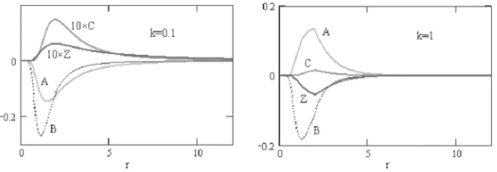
nega-tive. Examples of the solution to (3.4) for C and A are shown in Fig. 2. The amplitudes with n 1$ generally have a maximum at a finite radius.
4. Differential rotation
In the previous paper (Takahashi 2013), by neglecting the pressure gradient, i.e., r.h.s. of (2.3a) and . r nr 1 0 M 2 2 + . ~ ~ a~
-f
p
. C 1r C 2 n Cr 0 2 2 . a~ + + -m l c m , C r^ h.Jn^ a ~rhFig. 2 Examples of the solution for A and C with arbitrary unit. Figure on each curve is the value of a. Parameters are chosen as n = 1, ~ =-2.
(2.3b), the existence of perturbation with non-rigid phase rotation was suggested. In this section, we
shall take those pressure gradient terms into consideration to make the previous analysis more accu-rate.
The perturbations obey the equations (2.3a~c) together with the continuity equation (3.1). Now, we assume that the angular velocity ~ in (2.4a~d) is r-dependent, thereby yielding a differential
rota-tion. This assumption emerges from the fact that the time differentiation is always accompanied with the r-dependent angle-differentiation term. The amplitudes may also be assumed to be r-dependent
and have a common factor eikz as e.g. v Ae
r= i n r t ikz
d ^i-~^h h+ , dv =iBei n r t+ikz
i ^i-~^h h , dvz=iZei n^i-~^r th h+ikz
etc. Substituting these to (2.3a~c) and (3.1), we have
(4.1a) (4.1b) (4.1c) (4.1d) Owing to the appearance of the terms linear in t in (4.1a) and (4.1d), the density amplitude D will have a linear-dependence on t like
D=D0+iD1t. (4.2)
Of course, the phase of D1 must be chosen so as to keep the sign of the density positive. (4.1b~d)
show that, when A, B, C and Z are time-independent, D1 is non-zero only when A is non
-zero. Namely, the radial component of the velocity brings about in- or out-flow of matter and causes
the change in density for 2-dimensional flow.
B, C and Z are eliminated to get an equation involving A, D0, D1 and ~. Derivation of this
equa-tion is given in Appendix. Interestingly, this equaequa-tion involves only A and ~ and expresses that the product of A with a polynomial of ~ is zero. When A is non-zero, this equation leads to an
‘eigen-value’ equation for ~ :
(4.3) where ~u has been defined below Eq.(3.5). See Appendix for the derivation of (4.3). When k2 is
real and ~ is a solution of (4.3), its complex conjugate ~* is also a solution. In addition, (4.3) is invariant under n→-n, ~ →-~. This means that, if ~ is a solution for an n then -~ is a solution for -n.
Solutions for special values of n and k are given below.
v 2v v , n r A r B+ = C +i tC r D2 ~- i i - ~ - i l l a k v v , n r B+v + r A= n Cr ~- i -i i l a k a k v , n r Z= kC ~- i -a k v 0. iDo a+~-n r D r A A i tA rik +1 + l-~l -n B kZ- = v v v 4 4 0, r nr r r1 n k 4 2 2 2 3 3 2 2 2 2 4 + = ~- i ~- i ~ -i u u u c m
i) n=0 (unstable for k≠0)
(4.4) ii) n " 3; ; (unstable)
(4.5) iii) k=0 (unstable for n; ;$2 )
(4.6) Here, a mode of a complex ~ is called unstable. As is suggested by these extreme cases, the eigen-value equation (4.3) has both real and complex solutions for almost all regions of parameters. Two complex solutions are mutually complex conjugate. Therefore the perturbation blows up in course of time for one complex solution and decays for the other. The numerical solutions of (4.3) are
v . k r r 2 4 2 2 ! ! = + ~u i v . n r "! ! ~u i v or v . n r n r 1! 1 1! 1 = + ~u ^ h i ^- - h i
Fig. 3 Real (left) and imaginary (right) parts of four ~ as functions of r for n=1(upper panels) and 2 (lower panels), c=0.1, k=0.1. Two of the ~’s are real and the others are complex above the bifurcation point. The bifurcation point is inversely proportional to k. For n=2, ~’s with the smallest real part
shown in Fig. 3 for kz=0.1 and n=1 or 2. Errors of a few percent may exist when two branches are
contiguous.
Generally, there exist four distinct solutions. The sign of nRe(~) is positive or negative, corre-sponding to the mode that propagates positive or negative θ-direction, respectively. ~ with positive
imaginary part causes a temporal blow up of the oscillations in velocity field and other physical quan-tities. The mode with real ~ is of neutral stability. ~ with negative imaginary part corresponds to a decaying turbulence. We may call these three modes as growth, stationary and contraction mode, respectively. There exist regions of r where all frequencies are real. In these regions, four modes can coexist for a long term. It is also noted that the profile of Re~ is similar to that of vi.
We have seen that the complex ~’s are allowed for inviscid flow within linear perturbation where no constraint other than the equations of motion has been imposed on the perturbation. Nevertheless, the concept of NEIV will be a good approximation for real flows of a very large scale like typhoons. Let us assume that, for such flows, the space-dependent complex eigenvalues found above
are good approximation for temporal behaviours of perturbations. Now, the system’s energy can generally change in accordance with the variations of the velocities, pressure and density. Grow of amplitudes in viscous fluid will require addition of energy. Then, we may expect for viscous flows, when energy is added to the system in any form, the growth modes with Im ~>0 can be excited and the perturbations will grow. When there is no energy supply, the perturbation will decay. In this case the contraction modes with Im ~#0 will be of physical ones.
When k is real, the frequency generally acquires a nonzero imaginary part beyond a certain dis-tance. For surviving decay modes, it is rc=0 (n = 0) and rc=3 (n=1) in the above choice of
parame-ters. rc decreases as k increases. When k is complex, Im(~)!0 in the whole region of r. We will
consider the case of real k in the followings.
(4.1a~d) and (4.2) are not sufficient to determine the functional form of amplitudes. Instead, the ratios of amplitudes are given by the following relations (See Appendix for derivation) :
(4.7) (4.8) (4.9) From equations (4.7)~(4.9), together with the equation (A14) for A, the r-dependences of the
amplitudes are determined. The case for n=0 is shown in Fig. 4. All of the amplitudes shown here are real and have a peak near r=2. All of the perturbations are maximized inside the primary peak of
i v v , A B r n r 1 v 2 2 =~ - - i+~ i l uc u m v , A C r 2 = ~i u v . A Z k r 2 2 = ~ - i u
vi shown in Fig. 1.
Since vr and vz are zero for the unperturbed flow, the amplitudes A and Z are the direct measures of
the corresponding total (i.e., perturbed) velocity components. The r-dependences of vd r and vd z
determined by the amplitudes shown in Fig. 5 are shown in Fig. 6. The result for kz=1 are also
shown in the same figure. The direction of the flow changes drastically in the course of time. Simultaneous existence of vd r and vd z is a consequence of mass conservation in case no
singu-larity is present (Deppermen 1947).
In order to see the full profile of turbulences, we need to know the r-dependences of the amplitudes
Fig. 4 Perturbation amplitudes A, B, C and Z for real ~, n=0, kz=0.1 (left panel) and 1 (right panel). For
k=0.1, C and Z are magnified by ten-times. The sign of A is arbitrarily chosen.
Fig. 5 Perturbed dvr (upper left) and dvz (upper right) derived from the amplitudes shown in Fig. 5. Three curves are the velocity profiles at t = -20 (thin solid curve), -10 (dotted curve) and 0 (thick solid curve). The lower left and lower right panels are velocity components for kz=1.
A, B etc. This will be achieved by exploiting, e.g., the equation of state that relates D0 in (4.2) to C
and solving the equations (4.1). Then, e.g. for vi, the following single-mode perturbation is utilized
to observe the total circular flow profile :
(4.10) Other components are expressed in a similar way.
The immediate conclusion derived from (4.10) is that the turbulences propagate with the phase velocity given by
(4.11) The radial phase velocity does not have a unique definition. Here in (4.11), the radial component has been defined by a condition Re(~)t be temporary constant. The n = 0 mode does not propagate in azimuthal direction. The above result implies that the turbulences can in principle propagate to any directions, depending on the signs of Re(~), n and Re(k). In particular, the radial component is negative for t < 0 and positive for t > 0. Since the profile of Re(~) is similar to that of the azimuthal
vi,tot= +vi Re iBe6 i n^i+kz-~th@. , , . Re Re Re Re Re t n r k ~ ~ ~ ~ -l ^ ^ ^ ^ ^ e hh h hh o
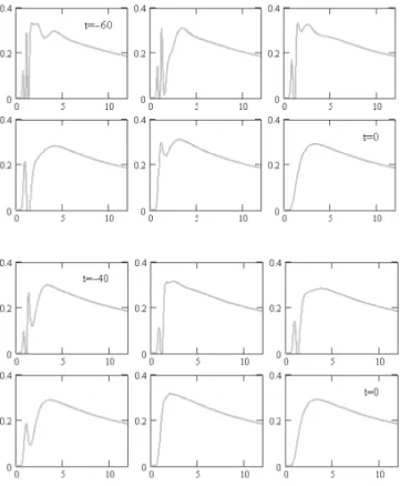
Fig. 6 Upper two rows : An example of the temporal variation of vi,tot given by (4.9) from t = -60 to 0 (from
top left to bottom right; from left to right) for n = 0, k = 0.1, c = 0.1, i = 0, z = 0. Amplitude was cho-sen arbitrarily. Lower two rows : k = 1 ; from t = -40 to 0. Other parameters are same as the upper two rows.
component, this means that the secondary peak moves first inward and later outward in the outer region. In the core, the motion is opposite. In contrast to the Rossby wave, the direction of the phase velocity is not affected by the Coriolis force.
In the calculations below, the amplitude A is chosen as a solution of (A14) with D0=0 for
conve-nience. An example of the temporal behaviour of vi,tot at i = 0 is shown in Fig. 6 for n=0,
k = 0.1. Here a real ~ has been chosen. At fixed time, several peaks appear due to the factor e-l r t~^ h.
The number of peaks is greater for larger maximum of ~(r). As was expected, the peaks in the region ~l<0 move inward when t < 0. Oppositely those in the region ~l < 0 move outward. In other words, the perturbation climbs up the slope of vi. The perturbation climbs down the slope of vi when t > 0. The case of k = 1 is also shown in Fig. 6.
In Fig. 6, more than one peak existed initially. For smaller k, the profile of peaks of vi is finer.
The outer peaks moves inward in course of time and disappear at t = 0. Since n = 0, the modulation at i = r from the unperturbed vi is in-phase with that of i = 0. In the case of k = 0.1, a fine structure
is observed as compared with the case of k = 1. Weakening and intensifying are taking place alter-nately at a fixed point.
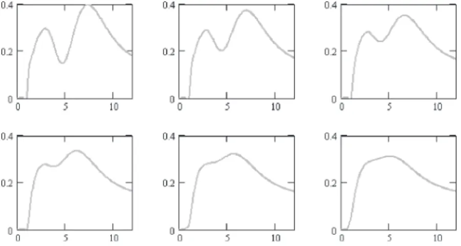
An example of n = 1 and Im #~ 0 is shown in Fig. 7. Im~ is nonzero for r > 3 (see Fig. 3). It is observed that initially one prominent secondary peak is present at around r = 7 and moves inward until it merges with the primary peak. During this change, the heights of the peaks get lower.
The difference between the two cases shown respectively in Fig. 6 and Fig. 7 is that, for n = 0, ~ is real and the motion at fixed r is periodic in time thereby yielding the same profiles repeatedly, while, for n = 1 (rc = 3), Im~ is negative in the region r > rc and the initial turbulences located beyond rc
decay exponentially. Although not shown here, after t = 0, the turbulences substantially disappear beyond the primary peak of vi. Even in this case, small turbulences generally remain and
periodi-cally repeat the appearance and disappearance in the region where Im(ω) is zero. The region where the turbulence is observed for a long time span diminishes as k gets larger. The long-time turbulence
is further suppressed for complex k.
As was mentioned before, the turbulence around the NEIV does not conserve but increases the energy. Thus an input of energy is a requisite for the excitation of the growth mode, which should be followed by the stationary and contraction modes after cutting off the supply of energy.
Two three-dimensional flow profiles are shown in Fig. 8. A concentric structure and a spiral
struc-ture of the eye wall are clearly observed in the mode n = 0 and 1, respectively. Also in the latter case, the double wall is observed in almost all radial directions.
Fig. 7 An example of the temporal variation of vi,tot given by (4.9) from t = -60 to 0 with equal time
inter-vals (from top left to bottom right ; from left to right) for n = 1, k = 0.1, c = 0.1 , i = 0, z = 0 and for a certain choice of amplitude.
Fig. 8 Three-dimensional flow profiles vi,tot for r < 9 at t = -50. Left : bird’s eye view, Right : view from a point on the polar axis. Model parameters for upper panels : n=0, k=0.1 and for lower panels : n=1,
5. Summary and remarks
In this paper, two kinds of perturbations around the axisymmetric NEIV are considered. In the per-turbation of the first kind, turbulences of the flow velocity, the pressure and the density are periodic in
i and t. They propagate azimuthally but not radially. The angular velocity of the azimuthal
propa-gation is real and constant. Turbulence rotates as if it were a rigid body. Obviously, this kind of perturbations must be of a small spatial scale.
In the perturbation of the second kind, the angular velocity is generally complex and is a function of the radial coordinate, thereby rendering the temporal behaviour aperiodic. The gross r-dependence
of the angular momentum is similar to that of vi^ hr . Thus, this kind of perturbations can be of a
large scale. Together with relatively high oscillations in radial direction, there can appear a promi-nent peak of turbulence beyond the primary maximum of vi. With the lapse of time, it moves inward
and disappears if the imaginary part of the angular momentum is negative. On account of the requi-site compressibility, both kinds of perturbation are of the density waves.
These results based on (3.4) and (4.3) do not depend on the functional form of the concentric flow,
r vi^ h.
It seems worthwhile to notice a striking similarity of the starting flow solution to the typhoon mod-els. Our analysis is based on the NEIV generated by barotropic balance. There rvi^ h is very small
near the symmetry axis, rapidly increases with r, takes a maximum at a certain radius and then mono-tonically decreases to zero as lnr/r. This behaviour of the azimuthal velocity is similar to the hori-zontal wind profiles of the typhoon models (Fujita 1952, Holland 1980, Merrill 1984, DeMaria 1987, Emanuel 2004, Holland et al. 2010) developed from the modified Rankine vortex model (Hughes 1952). The distinctive features of our vi^ hr is that it has an ‘eye’ at the center and exhibits non
-power decay at long distances, which is also in agreement with the observations. This indicates that the thermally averaged intermediate level profile of typhoon can be understood in terms of the Newto-nian mechanics. It is known that the track of typhoon predicted by a model calculation is sensitive to the form of rvi^ h (Holland and Leslie 1995). Utilizing the flow profile given by vi in the calculation
of typhoon track will be intriguing.
Unfortunately, the perturbations vd r and vd z obtained in the previous sections are strongly
oscillat-ing in time and do not reproduce observations on real typhoon. In reality, vd r is negative and v;d r;
is an increasing function of r outside the primary peak of vi where a convection ring exists (Depperman
wind, which is of course constrained of having zero upward velocity at the sea surface. Thus it will be worthwhile to explore what occurs to vd r and vd z if physically meaningful boundary conditions are
taken into account, which is an entirely non-trivial problem because ~ is complex, albeit non-
vanish-ing vd r and vd z are also a consequence of temperature difference between the core and environments
in real typhoon (Depperman 1947). Namely, in our scheme of purely Newtonian dynamics (i.e., no thermodynamical effects being taken into account), one may envisage the system to be closed down-ward and be open updown-ward. Then, the existences of flow in indown-ward radial direction and the peak in vi
at some radius, together with the continuity, will solely imply an emergence of a convective ring. It is also notable that real typhoons sometimes exhibit the second peak (and in some cases, the third peak, too) of rvi^ h. There are many hypotheses proposed so far to explain the formation of the
sec-ondary eyewall (See e.g., Terwey and Montgomery 2008). One of the characteristic of the secsec-ondary eyewall is its inward movement (see e.g., Willoughby et al. 1989). Such a behaviour of turbulence might be interpreted as the perturbation of the second kind discussed in this paper, provided that the secondary peak is associated with a strong upflow under realistic boundary conditions. Willoughby et al. (1989) reported that the region of turbulence formed a circle or semicircle. In our terminology, this phenomenon is interpreted that the mode of n = 0 or 1 dominated. Higher modes will possibly be excited, too.
It should be kept in mind that, in reality, the formation and movement of the second peak in azi-muthal velocity occur through the life cycle of typhoon. In particular, the merge of two peaks seems to mark the period of transition from typhoon to tropical cyclone. In our view, this process will cor-respond to the complex ~ with a negative imaginary part. Confirming further the applicability of our model to the real typhoon will require analyses that take account of the variations of such model parameters as c and c1 as well as the superposition of modes that fulfill given boundary conditions.
The perturbation associated with a vortex of a planetary scale has been known as the Rossby wave. The essential point of the emergence of this wave is the interaction of the vorticity with the rotation of the earth. The phase velocity of the Rossby wave is determined through the relation of the back-ground flow with the Coriolis force. In contrast, the perturbations we explored in the present paper do not depend on the Coriolis force and propagate to any directions with the space-time dependent
velocity determined by the background velocity field together with the mode. Future advance in observation will enable to judge the existence of the wave of this kind in typhoons or hurricanes.
Appendix : Eigenfrequency equation
In this Appendix, starting from (4.1) and (4.2) in the main text, the equation is derived that deter-mines the r-dependence of the frequency ~. Note that explicitly t-dependent terms exist in (4.1a)
and (4.1d). These terms must be cancelled by similar t-dependent terms involved in D. Then this
kind of cancellations take place when
(A1) (A2) where ~u/~-n rvi/ . By comparing t0 terms in (4.1a~d), we obtain
(A3) (A4) (A5) (A6) Eliminating D1 from (A1) and (A2), we have
(A7) (A6), (A3) and (A1) form the set of differential equations
(A8) (A9) (A10) where (A5) has been used to eliminate Z. Remaining equations (A4) and (A7) are the constraints that are used to express B and C in terms of A :
(A11) (A12) Dividing both sides of these equations by A, together with (A.5), we have (4.6), (4.7) and (4.8) in the main text.
Differentiating both sides of (A12) with respect to r leads to
(A13) 0, C vr D2 1= ~ - i l , D1 A 0 ~u -~l = 2 , A+ r Bv = C vr D2 0 ~ i - - i l u i , B+v +vr A= n Cr ~u a l ik -, Z kC ~u = . D1-~uD0-1r A A- +l n B kZr + =0 0. C vr A2 = ~u - i , A 1r A rn B D1 D0 k C 2 ~ ~ =- + + - + l u u 2 , Cl= ~-uA- r Bvi -vr Di2 0 , A D n rv 1 = ~ ~ - i l l u u a k i , B 1 v vr n vr A2 2 =-~ + i+~ i l uc u m . C=r Av2 ~ i u . Cl=r Av~i2 l+ vr~i2 lA u c um
(A2), (A11) and (A12) can be used to express Al in (A8) and Cl in (A9) in terms of A and D0 as
(A14)
(A15)
On the other hand, by using (A14), we eliminate Al in (A13) to obtain
(A16) Equating (A16) to (A15), D0 disappears and only A remains. Then, assuming that A is nonzero, we
have the equation (4.3) in the main text.
References
Arnol’d V I 1965a : Conditions for nonlinear stability of stationary plane curvilinear flows of ideal flui. Dokl. Akud. Nauk, SSSR 162 97 [trans. in Soviet Math. 6 773-777 (1965)].
Arnol’d V I 1965b : Variational principle for three-dimensional steady-state flows of an ideal fluid. Prikl. Math. I Mech. 29 846 [transl. J. Appl. Math. Mech. 29 1002-1008 (1965)].
Burgers J M 1948 : A mathematical model illustrating the theory of turbulence. Adv. Appl. Mech. 1 171. DeMaria M 1987 : Tropical cyclone track prediction with a barostropic spectral model. Mon. Wea. Rep.
115 2346.
Depperman C E 1947 : Notes on the origin and structure of Philippine typhoon. Bull. Amer. Meteor. Soc.
28 399-404.
Drazin P and Riley N 2006 : The Navier-Stokes Equations A Classification of Flows and Exact Solutions
Cambridge Univ. Press (Cambridge).
Emanuel K A 2004 : Tropical cyclone energetics and structure. Atmospheric Turbulence and Mesoscale Meteorology, Federovich E et al (eds) Cambridge Univ. Press (Cambridge), 165-192.
Fujita T 1952 : Pressure distribution within a typhoon. Geophys. Mag. 23 437-451. Hocking L M 1963 : An example of boundary layer formation. AIAA J. 1 1222.
Holland G J 1980 : An analytic model of the wind and pressure profiles in hurricanes. Mon. Wea. Rev. 108 1212-1218.
Holland G J and Leslie L M 1995 : On the bogussing of tropical cyclones in numerical models : a com-parison of vortex profiles. Meteorol. Atomos. Phys. 56 101-110.
Holland G J, Belanger J I and Fritz A 2010 : A revised model for radial profiles of hurricane winds. Mon. Wea. Rep. 138 4393 and references cited therein.
Merrill R T 1984 : A comparison of large and small tropical cyclones Mon. Wea. Rep. 112 1408. Preston J H 1950 : The steady circulatory flow about a circular cylinder with uniformly distributed suction
at the surface. Aeronaut Q. 1 319.
Takahashi K 2013 : Vorticity equation, current conservation and the solutions of the Navier-Stokes equa-tion. Facul. Lib. Arts Rev. (Tohoku Gakuin Univ.) www.tohoku-gakuin.ac.jp/research/journal/ bk2013/no01.htm
Terwey W D and Montgomery M T 2008 : Secondary eyewall formation in two idealized, full-physics modeled hurricanes. J. Geophys. Res. 113 D12112.
Vallis G K, Carnevale G F and Young W R 1989 : Extremal energy properties and construction of stable solutions of the Euler equations. J . Fluid Mech. 207 133.
2 , A 1r n rv2 n vr3 k vr A A D 2 2 2 2 0 = + + ~ ~ ~ ~ ~ ~ - i- i - i -l c uc u m u m uul u i 2 . C v vr vr n vr2 A vr D 2 2 0 =-~-~i + i+~ i - i l cu u c l u mm 2 . C rv2 1r n rv2 n vr3 k vr A A D vr A 2 2 2 2 0 2 = ~ +~ ~ + + ~ ~ ~ ~ ~ - - - -i i i i i l u; c uc u m u m uul u E c u ml
Willoughby H E, Clos J A and Shoreibah M G 1982 : Concentric eye walls, secondary wind maxima, and the evolution of the hurricane vortex. J. Atmos. Sci. 39 395.