Vol. 52, No. 2 (2016), 193–214
Improved transformation of ϕ-divergence
goodness-of-fit test statistics based on minimum
ϕ
∗-divergence estimator for GLIM of binary data
Nobuhiro Taneichi, Yuri Sekiya and Jun Toyama
(Received September 16, 2016; Revised November 14, 2016)
Abstract. Generalized linear models of binary data including a logistic
regres-sion model and a probit model are considered. For testing the null hypothesis that the considered model is correct, the ϕ-divergence family of goodness-of-fit test statistics Cϕϕ∗ that is based on a minimum ϕ∗-divergence estimator is
considered. The family of statistics Cϕϕ∗includes a power divergence family of
statistics Ra,b that is based on a minimum power divergence estimator. The derivation of an expression of a continuous term of asymptotic expansion for the distribution of Cϕϕ∗under the null hypothesis is shown. Using the
expres-sion, a transformed Cϕϕ∗ statistic that improves the speed of convergence to
the chi-square limiting distribution of Cϕϕ∗is obtained. In the case of Ra,b, it is
numerically shown that the transformed statistics usually perform better than the original statistics with respect to speed of convergence to the chi-square limiting distribution and it is also numerically shown that the power of the transformed statistics is almost the same as that of the original statistics.
AMS 2010 Mathematics Subject Classification. 62E20, 62H10.
Key words and phrases. Asymptotic expansion, binary data, ϕ-divergence
statistics, generalized linear model, improved transformation, minimum ϕ∗ -divergence estimator.
§1. Introduction
We discuss generalized linear models (Nelder and Wedderburn [10]) in which the response variables are measured on a binary scale. Let N independent random variables Yα, α = 1, . . . , N corresponding to the number of successes
in N different subgroups be distributed according to binomial distributions
B(nα, πα), α = 1, . . . , N. If we use a monotone and differentiable function g
as a link function, we obtain a generalized linear model for binary data as 193
follows.
(1.1) g(πα) = x′αβ (α = 1, . . . , N ),
where xα = (xα1, . . . , xαp)′(α = 1, . . . , N ) are covariate vectors and β =
(β1, . . . , βp)′ is an unknown parameter vector and p < N . We consider a
mini-mum ϕ∗-divergence estimator of model (1.1) and also consider a ϕ-divergence goodness-of-fit test statistic based on the estimator. Let yα (α = 1, . . . , N )
be an observed value of Yα (α = 1, . . . , N ), then the minimum ϕ∗-divergence
estimator of model (1.1) is given by ˆ βgϕ ∗ = arg min β∈Θ Dϕ∗, where Dϕ∗ = 1 N N ∑ α=1 nα πα(β)ϕ ∗ yα nα πα(β) + (1 − πα(β))ϕ∗ 1− yα nα 1− πα(β) , where ϕ∗ is a real convex function in (0,∞) satisfying ϕ∗(1) = ϕ∗′(1) = 0, ϕ∗′′(1) = 1, 0ϕ∗(0/0) = 0, 0ϕ∗(x/0) = limu→∞ϕ∗(u)/u, and Θ is an
open subset of Rp (Pardo [11]). When we choose a convex function
(1.2) ϕa(t) =
{a(a + 1)}−1{ta+1− t + a(1 − t)} (a ̸= 0, −1)
t log t + 1− t (a = 0)
− log t − 1 + t (a =−1),
as ϕ∗(t), Dϕ0 becomes a Kullback divergence measure (Kullback [7]). Then, in
this case, estimator ˆβgϕ0 becomes the maximum likelihood estimator. There-fore, the maximum likelihood estimator is a special case of the minimum ϕ∗ -divergence estimator.
In order to test the null hypothesis
(1.3) H0g: πα= πα(β) = g−1(x′αβ) (α = 1, . . . , N ),
we consider the family of ϕ-divergence statistics based on the minimum ϕ∗ -divergence estimator (1.4) Cϕϕ∗ = 2 N ∑ α=1 nα πˆgϕ ∗ α ϕ nYαα ˆ πgϕα ∗ + (1 − ˆπgϕ∗ α )ϕ 1− Ynαα 1− ˆπgϕα ∗ , where ˆπαgϕ∗ = πα( ˆβ gϕ∗ ) (α = 1, . . . , N ), ˆβgϕ∗ = ( ˆβ1gϕ∗, . . . , ˆβpgϕ∗)′ is the
same conditions of ϕ∗ (Pardo [11], Pardo and Pardo [12]). The test statistic
Cϕ given by (7) in Taneichi et al. [21] is written as Cϕ≡ Cϕϕ0, and therefore
the family of statistics given by (1.4) includes that of Cϕ.
When we choose convex functions ϕa and ϕb given by (1.2) as ϕ and ϕ∗,
respectively, in (1.4), Cϕaϕb becomes a power divergence statistic
(1.5) Ra,b= 2 N ∑ α=1 nα { Ia ( Yα nα , ˆπgϕb α ) + Ia ( 1−Yα nα , 1− ˆπgϕb α )} , where Ia(e, f ) = {a(a + 1)}−1e{(e f )a − 1} (a̸= 0, −1) e log ( e f ) (a = 0) f log (f e ) (a =−1),
which is based on the minimum power divergence estimator (Cressie and Read [4], Read and Cressie [14]). Under H0g, all members of the class of statistics
Cϕϕ∗ have a χ2N−p limiting distribution, assuming the condition that (1.6) nα/n→ µα(α = 1, . . . , N ) as n→ ∞,
where n = ∑Nα=1nα, 0 < µα < 1 (α = 1, . . . , N ) and
∑N
α=1µα = 1. Using
the results, we can use Cϕϕ∗ as a goodness-of-fit test statistic for model (1.1).
With regard to the goodness-of-fit test for a multinomial distribution, Yarnold [23] obtained an approximation based on asymptotic expansion for the null distribution of Pearson’s X2 statistic. The expansion consists of a term of multivariate Edgeworth expansion for a continuous distribution and a discontinuous term. In a fashion similar to that for Pearson’s X2 statis-tic, approximations based on asymptotic expansions for null distributions of some kinds of multinomial goodness-of-fit statistics have been investigated by Siotani and Fujikoshi [16], Read [13] and Men´endez et al. [9]. Edgeworth approximations of the distributions of some kinds of multinomial goodness-of-fit statistics under alternative hypotheses have also been investigated by Taneichi et al. [17, 18], and Sekiya and Taneichi [15]. Taneichi and Sekiya [19] discussed approximations for the distribution of ϕ-divergence statistics for the test of independence in r× s contingency tables. By using the above the-ory of approximation, Taneichi et al. [21] considered a family of ϕ-divergence statistics using the maximum likelihood estimator Cϕ≡ Cϕϕ0 and investigated
asymptotic approximation of the distribution of statistics for testing the null hypothesis H0g given by (1.3). They proposed transformed Cϕ statistics that
improve the speed of convergence to a chi-square limiting distribution. In this paper, we generalize the family of statistics Cϕ ≡ Cϕϕ0 based on
ϕ-divergence to Cϕϕ∗ and investigate an asymptotic approximation of the
In Section 2, we first describe a local Edgeworth approximation for the prob-ability of Yα (α = 1, . . . , N ) under H0g. Next, we consider an expression of
asymptotic expansion for the distribution of Cϕϕ∗ under H0g. Evaluation for the continuous term of the expression is considered. In Section 3, using the term of multivariate Edgeworth expansion assuming a continuous distribution in the expression in Section 2, we construct transformations for improving small-sample accuracy of the χ2 approximation of the distribution of Cϕϕ∗
under H0g. In Section 4, in the case of Ra,b, performance of the transformed statistic and that of the original statistic are compared numerically.
§2. Asymptotic approximation for the distribution of Cϕϕ∗
under H0g
First, we consider a local Edgeworth approximation for the probability of
Yα (α = 1, . . . , N ) under null hypothesis H0g given by (1.3). Let Yα, α =
1, . . . , N be distributed according to a binomial distribution B(nα, παg) α =
1, . . . , N, where each παg (α = 1, . . . , N ) is represented as παg = g−1(x′αβ) (α =
1, . . . , N ) by using covariate vectors xα = (xα1, . . . , xαp)′ and an unknown
parameter vector β. Let
(2.1) Wα=
Yα√− nαπαg
nα
(α = 1, . . . , N ).
Then, W = (W1, . . . , WN)′ is a lattice random vector that takes values in the
set L = { w = (w1, . . . , wN)′ : wα= yα− nαπ g α √ nα (α = 1, . . . , N ), y = (y1, . . . , yN)′ ∈ M } , where M = {
y = (y1, . . . , yN)′ : y1, . . . , yN are non-negative integers that satisfy yα≤ nα (α = 1, . . . , N )
}
.
If we consider only for a limiting distribution of Cϕϕ∗, we can discuss under
the assumption given by (1.6). In this section, since we consider asymptotic expansion of the distribution of Cϕϕ∗, we need an assumption that states the
way of converging nα/n to µα more strictly than the assumption given by
assumption given by (1.6).
Assumption 2.1. nα → ∞ (α = 1, . . . , N), as n → ∞, with nαdepending on
n in such a way that nα/n = µα (α = 1, . . . , N ), where 0 < µα < 1
(α = 1, . . . , N ) and ∑Nα=1µα = 1.
With regard to a local Edgeworth approximation for the probability of
Yα (α = 1, . . . , N ) under H0g, the following lemma is shown in Taneichi et al. [21].
Lemma 2.1. For each y = (y1, . . . , yN)′ ∈ M, let w = (w1, . . . , wN)′, where
wα = (yα− nαπgα)/√nα (α = 1, . . . , N ). Then, under Assumption 2.1,
Pr{W = w|H0g} = ( N ∏ α=1 1 √ nα ) hg(w) { 1 +√1 nh g 1(w) + 1 nh g 2(w) + 1 n√nh g 3(w) + O(n−2) } , where (2.2) hg(w) = (2π)−N/2|Ω|−1/2exp ( −1 2w ′Ω−1w), hg1(w) = −1 2 N ∑ α=1 1 √ µα 1− 2παg παg(1− παg)wα+ 1 6 N ∑ α=1 1 √ µα 1− 2παg (παg)2(1− πgα)2w 3 α, hg2(w) = 1 2{h g 1(w)}2− 1 12 N ∑ α=1 1 µα 1− παg + (πgα)2 παg(1− παg) +1 4 N ∑ α=1 1 µα 1− 2πgα+ 2(πgα)2 (παg)2(1− παg)2 w 2 α − 1 12 N ∑ α=1 1 µα 1− 3παg + 3(πgα)2 (παg)3(1− παg)3 w 4 α, hg3(w) = −1 3{h g 1(w)} 3+ hg 1(w)h g 2(w) + 1 12 N ∑ α=1 1 µα√µα 1− 2πα (παg)2(1− παg)2wα −1 6 N ∑ α=1 1 µα√µα (1− 2πgα)(1− πgα+ (παg)2) (παg)3(1− πgα)3 w 3 α + 1 20 N ∑ α=1 1 µα√µα (1− 2παg)(1− 2παg + 2(παg)2) (πgα)4(1− παg)4 w 5 α,
and
(2.3) Ω = diag(π1g(1− πg1), . . . , πgN(1− πgN)).
For the statistics Cϕ ≡ Cϕϕ0, Taneichi et al. [21] considered the following
approximation for the distribution of Cϕunder H0g.
Pr{Cϕ≤ x|H0g} ≈ J1g,ϕ(x) + J2g,ϕ(x),
where the J1g,ϕ(x) term is multivariate Edgeworth expansion assuming a con-tinuous distribution and the J2g,ϕ(x) term, which corresponds to the K2 term of Taneichi et al. [17] in the case of a multinomial goodness-of-fit test, is a discontinuous term to account for the discontinuity. By using the continuous term J1g,ϕ(x), a transformation for Cϕthat improves the speed of convergence
to a χ2 limiting distribution is constructed. Let Jg,ϕϕ∗
1 (x) be a continuous term of the approximation of Pr{Cϕϕ∗ ≤ x|H0g}. Similarly, in this paper, we
construct the transformation for Cϕϕ∗ by using Jg,ϕϕ
∗
1 (x). With regard to evaluation of the J1g,ϕϕ∗(x) term, we obtain the following theorem.
Theorem 2.1. When g−1 and ϕ∗ are fourth time continuously differentiable functions and ϕ is a fifth time continuously differentiable function, under
As-sumption 2.1, the J1g,ϕϕ∗(x) term is evaluated as
(2.4) J1g,ϕϕ∗(x) = Pr{χ2N−p ≤ x} + 1 n 3 ∑ j=0 vg,ϕϕj ∗Pr{χ2N−p+2j≤ x} + O(n−2), where χ2
f denotes a chi-square random variable with degrees of freedom f ,
v0g,ϕϕ∗ = 1 24(−Γ4), v1g,ϕϕ∗ = 1 24 [ Γ1ϕ(4)(1) + Γ2{ϕ ′′′ (1) + 1}2+ (2Γ1+ Γ3)ϕ ′′′ (1) +(Γ3+ Γ4) + ∆ ] , vg,ϕϕ2 ∗ = 1 24 [ −Γ1ϕ(4)(1)− 2Γ2{ϕ′′′(1) + 1}2− (2Γ1+ Γ3)ϕ ′′′ (1)− Γ3− ∆ ] , v3g,ϕϕ∗ = 1 24Γ2{ϕ ′′′(1) + 1}2, where ∆ = Γ5{ϕ∗ ′′′ (1) + 1}{ϕ∗′′′(1)− 2ϕ′′′(1)− 1},
Γ3 = 2(3A1− 2A2− 6A3+ 6A4+ 3A5+ 3A6− 6A7− 3A8− 3B3+ 2B4+ 3B8), Γ4 = 6A1− 4A2− 6A6+ 12A8− 3A9+ 4B4− 12B5+ 6B6− 3B9, Γ5 =−3(2A4− 4A7+ B1− 2B2+ 2B4+ B7), A1 = N ∑ α=1 1− 3παg + 3(παg)2 µαπαg(1− παg) , A2 = N ∑ α=1 (1− 2παg)2 µαπαg(1− παg) , A3 = N ∑ α=1 1− 3πgα+ 3(παg)2 (παg)2(1− παg)2 G1(α)2σαα, A4 = N ∑ α=1 (1− 2παg)2 (πgα)2(1− παg)2 G1(α)2σαα, A5 = N ∑ α=1 1− 2παg πgα(1− παg) G2(α)σαα, A6 = N ∑ α=1 µα(1− 3πgα+ 3(παg)2) (παg)3(1− πgα)3 G1(α)4σ2αα, A7= N ∑ α=1 µα(1− 2πgα)2 (παg)3(1− παg)3 G1(α)4σαα2 , A8 = N ∑ α=1 µα(1− 2παg) (πgα)2(1− παg)2 G1(α)2G2(α)σαα2 , A9 = N ∑ α=1 µα παg(1− παg) G2(α)2σ2αα, B1 = N ∑ α=1 N ∑ γ=1 1− 2πgα παg(1− πgα) 1− 2πγg πγg(1− πgγ) G1(α)G1(γ)σαγ, B2 = N ∑ α=1 N ∑ γ=1 µα(1− 2παg) (παg)2(1− παg)2 1− 2πγg πgγ(1− πγg) G1(α)3G1(γ)σαασαγ, B3= N ∑ α=1 N ∑ γ=1 µα παg(1− παg) 1− 2πγg πγg(1− πγg) G1(α)G2(α)G1(γ)σαασαγ, B4 = N ∑ α=1 N ∑ γ=1 µα(1− 2πgα) (παg)2(1− πgα)2 µγ(1− 2πgγ) (πγg)2(1− πgγ)2 G1(α)3G1(γ)3σ3αγ, B5= N ∑ α=1 N ∑ γ=1 µα παg(1− παg) µγ(1− 2πγg) (πgγ)2(1− πγg)2 G1(α)G2(α)G1(γ)3σαγ3 , B6= N ∑ α=1 N ∑ γ=1 µα παg(1− παg) µγ πγg(1− πγg) G1(α)G2(α)G1(γ)G2(γ)σαγ3 , B7 = N ∑ α=1 N ∑ γ=1 µα(1− 2παg) (πgα)2(1− παg)2 µγ(1− 2πγg) (πgγ)2(1− πγg)2 G1(α)3G1(γ)3σαασαγσγγ,
B8 = N ∑ α=1 N ∑ γ=1 µα πgα(1− πgα) µγ(1− 2πγg) (πγg)2(1− πγg)2 G1(α)G2(α)G1(γ)3σαασαγσγγ, B9 = N ∑ α=1 N ∑ γ=1 µα πgα(1− πgα) µγ πgγ(1− πgγ) G1(α)G2(α)G1(γ)G2(γ)σαασαγσγγ, Gi(α) = u(i)(x′αβ) (α = 1, . . . , N, i = 1, 2), u(x) = g−1(x), σαγ= p ∑ l=1 p ∑ m=1 κl,mxαlxγm (α, γ = 1, . . . , N ), κl,m= N ∑ λ=1 µλ{πλg(1− πλg)}−1G1(λ)2xλlxλm (l, m = 1, . . . , p),
where u(i) is the i-th derivative of u and κl,m is the (l, m)-element of the
inverse matrix K−1 of K = (κl,m).
Proof of Theorem 2.1 is shown in Appendix. From Theorem 2.1, we can verify the following. The coefficients vg,ϕϕj ∗(j = 0, 1, 2, 3) satisfy the relation ∑3 j=0v g,ϕϕ∗ j = 0. The coefficients v g,ϕϕ∗ 0 and v g,ϕϕ∗
3 are not dependent on ϕ∗. When ϕ∗ = ϕ0, coefficients coincide with those for the family of statistics Cϕ
shown in Theorem 1 of Taneichi et al. [21].
If we apply ϕa as ϕ and ϕb as ϕ∗ in Theorem 2.1, we obtain the following
corollary for the statistic Ra,b based on power divergence.
Corollary 2.1. When the statistic is Ra,b given by (1.5) and g−1 is a fourth
time continuously differentiable function, under Assumption 2.1, the J1g,ϕϕ∗(x)
term is evaluated as J1g,ϕϕ∗(x) = Pr{χ2N−p ≤ x} + 1 n 3 ∑ j=0 vg,(a,b)j Pr{χ2N−p+2j≤ x} + O(n−2),
where vjg,(a,b)(j = 0, 1, 2, 3) are defined as vjg,ϕϕ∗ (j = 0, 1, 2, 3) in the case of
§3. Transformed statistics based on the Jg,ϕϕ∗
1 (x) term In this section, we first describe the idea of transformation for improving small-sample accuracy of χ2 approximation of the distribution of a random variable.
Suppose that a nonnegative random variable T has an asymptotic expansion such that Pr{T ≤ x} = Pr{χ2f ≤ x} + 1 n m ∑ j=0 ajPr{χ2f +2j ≤ x} + O(n−2),
where m is a positive integer. Also suppose that the coefficients aj (j =
0, 1, . . . , m) do not depend on the parameter n(> 0) and must satisfy the relation∑mj=0aj = 0.
For m = 1, in order to increase the accuracy of χ2 approximation of a random variable T , we consider transformed random variable TB defined by
(3.1) TB= ( 1 +2a0 f n ) T.
Then, it holds that
Pr{TB≤ x} = Pr{χ2f ≤ x} + O(n−2).
This result is known as a Bartlett adjustment. Lawley [8], Barndorff-Nielsen and Cox [2], and Barndorff-Nielsen and Hall [3] discussed Bartlett adjustment for the log-likelihood ratio statistic.
For m = 3, in order to increase the accuracy of χ2 approximation of a random variable T , we consider transformed random variable TI defined by
(3.2) TI = (nα + β)2log [ 1 + 1 (nα)2 { T + 1nα (T2+ γT3) + 1 (nα)2 ( 1 3T 3+3γ 4 T 4+ 9γ2 20 T 5 )}] ,
where α = −f(f + 2){2(a2 + a3)}−1, β = −(f + 2)a0{2(a2 + a3)}−1 and
γ = a3{(f +4)(a2+ a3)}−1. Then, it holds that
Pr{TI ≤ x} = Pr{χ2f ≤ x} + O(n−2).
The proof of the results for transformation of TI is given by Yanagihara [22].
The proof is derived by applying the idea of Kakizawa [6] to the theory of improved transformation given by Fujikoshi [5].
Applying the evaluation (2.4) given by Theorem 2.1 to the above trans-formed statistics TB given by (3.1) and TI given by (3.2), we construct
trans-formations for improving small-sample accuracy of the χ2 approximation of the distribution of Cϕunder H0g.
When ϕ and ϕ∗ satisfy
(3.3) ϕ′′′(1) =−1, ϕ(4)(1) = 2 and ϕ∗′′′(1) =−1,
equations v1g,ϕϕ∗ = −vg,ϕϕ0 ∗ and v2g,ϕϕ∗ = v3g,ϕϕ∗ = 0 hold in Theorem 2.1. Then, we can consider Bartlett-type adjustment
CϕϕB∗ = { 1 + 2v g,ϕϕ∗ 0 n(N− p) } Cϕϕ∗.
On the other hand, when ϕ does not satisfy (3.3), we can consider the transformed statistic CϕϕI ∗ = (nα + β)2log (1 + ζ) , where ζ = 1 (nα)2 [ Cϕϕ∗+ 1 nα{(Cϕϕ∗) 2+ γ(C ϕϕ∗)3} + 1 (nα)2 {1 3(Cϕϕ∗) 3+3γ 4 (Cϕϕ∗) 4+9γ2 20 (Cϕϕ∗) 5}], α =−(N −p)(N −p+2){2(v2g,ϕϕ∗+v3g,ϕϕ∗)}−1, β =−(N −p+2)v0g,ϕϕ∗{2(vg,ϕϕ2 ∗ +v3g,ϕϕ∗)}−1 and γ = v3g,ϕϕ∗{(N − p + 4)(vg,ϕϕ2 ∗+ vg,ϕϕ3 ∗)}−1.
Practically, we may use estimate ˆvjg,ϕϕ∗ (j = 0, 2, 3) obtained by substi-tuting minimum ϕ∗-divergence estimate ˆβgϕ∗ for true value β in vjg,ϕϕ∗ (j = 0, 2, 3). Therefore, when ϕ and ϕ∗ satisfy (3.3), we propose the statistic ˜CϕϕB∗
that is obtained by substituting ˆvg,ϕϕ0 ∗ for v0g,ϕϕ∗ in CϕϕB∗, that is,
(3.4) C˜ϕϕB∗ = { 1 + 2ˆv g,ϕϕ∗ 0 n(N− p) } Cϕϕ∗.
Similarly, when ϕ and ϕ∗ do not satisfy (3.3), we also propose the statistic ˜
CϕϕI ∗ that is obtained by substituting ˆvg,ϕϕ ∗
j (j = 0, 2, 3) for v g,ϕϕ∗
j (j = 0, 2, 3)
in CϕϕI ∗.
In the case of power divergence statistic Ra,b= Cϕaϕb using the minimum
and b = 0 (log likelihood ratio statistic). Then, we consider the transformed statistic given by (3.4) when a = 0 and b = 0 and put ˜R0,0B = ˜CϕB
0ϕ0. When the
link function g is a logit link function, statistic ˜R0,0B coincides with the statistic ˜
D proposed by (3.4) of Taneichi et al. [20]. On the other hand, we consider
statistic ˜CϕIaϕ
b when a̸= 0 or b ̸= 0 and put ˜R
a,b
I = ˜CϕIaϕb (a̸= 0 or b ̸= 0).
We summarize the difference and relation between TB and TI. Transformed
statistic TB is a simple monotone transformation of Cϕconstructed by a linear
function whose intercept is zero. On the other hand, transformed statistic TI is
a monotone transformation of Cϕconstructed by logarithm of quintic function.
It is much more complicated than TB. Then, from point of view of stability, TI
seems to be inferior to TB. However, for Cressie and Read family of statistics Ra,b, TB increases the speed of convergence to chi-square distribution only for
the statistic in the case of a = b = 0, that is, the log-likelihood ratio statistic. Therefore, for improving the other statistics, statistic TI is developed.
§4. Performance of transformed statistics
In this section, we compare the performance of transformed statistics ˜Ra,bI (a̸= 0 or b̸= 0) with that of the original power divergence statistics Ra,busing the minimum power divergence estimator by the Monte Carlo procedure. The performance of transformed statistic ˜R0,0B for complementary log-log link g0 and probit link gP is shown in Fig.1, Fig.2 and Fig.3 of Taneichi et al. [21].
We consider a generalized linear model given by (1.1) with p = 2 and xα1= 1
and xα2= xα (α = 1, . . . , N ).
Let the true values of parameters β1 and β2 be β1∗ and β2∗, respectively. Then, the true value of παg (α = 1, . . . , N ) is
(4.1) πgα∗= g−1(β1∗+ β2∗xα) (α = 1, . . . , N ).
As a link function g, we consider the family of link functions given by Aranda-Ordaz [1], g(t) = gc(t) = log { (1− t)−c− 1 c } ,
that depend on parameter c. gc include the logit link g1 and complementary log-log link g0 as a limit. We also consider the probit link gP(t) = Φ−1(t),
where Φ is the cumulative distribution function of a standard normal distri-bution.
We give a design matrix
X = (
1 · · · 1
x1 · · · xN
and execute the following procedure.
For each α, we generate nα (α = 1, . . . , N ) binomial random numbers
that are distributed according to B(1, παg∗) (α = 1, . . . , N ). From them, we
calculate the number of successes Yα (α = 1, . . . , N ) and the minimum ϕb
-divergence estimates ˆβgϕb
1 and ˆβ
gϕb
2 for the parameters β1 and β2. Using the estimates, we calculate the values πα( ˆβ
gϕb
) (α = 1, . . . , N ), where ˆβgϕb = ( ˆβgϕb
1 , ˆβ
gϕb
2 )′, and observed values of the statistics Ra,b, ˜R
a,b
I (a̸= 0 or b ̸= 0).
This process is repeated D times.
Among D times, let V be the number of times that the observed values of the statistic exceed the upper ε point of the χ2 distribution with degrees of freedom N − p, that is, χ2N−p(ε). The performance of χ2 approximation for the distribution of each statistic can be evaluated on the basis of the index
I = V
D − ε.
We consider the following two true parameters (i) β1∗=−0.1, β2∗= 0.1,
(ii) β1∗= 0.1, β2∗ =−0.1,
and investigate the performance of the following four cases of design matrix when N = 8. (I) X = ( 1 1 1 1 1 1 1 1 2.7 3.0 3.3 3.6 3.9 4.2 4.5 4.8 )′ . (II) X = ( 1 1 1 1 1 1 1 1 2.85 3.05 3.25 3.45 3.65 3.85 4.05 4.25 )′ . (III) X = ( 1 1 1 1
log(2.7) log(3.0) log(3.3) log(3.6)
1 1 1 1
log(3.9) log(4.2) log(4.5) log(4.8) )′ . (IV) X = ( 1 1 1 1
log(2.85) log(3.05) log(3.25) log(3.45)
1 1 1 1
log(3.65) log(3.85) log(4.05) log(4.25) )′
For each case, we consider a sample design n1 =· · · = n8= n∗.
We investigate the performance for all combinations of the two true param-eters (i) and (ii), four design matrices (I), (II), (III) and (IV), and the sample design with n∗ = 20. Some of the results of the investigations are shown in figures as follows.
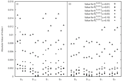
Fig.1 shows the absolute values of index I when the test statistic is R0.2,0.2 and models are given by link functions g0 (complementary log-log model),
g1/2, g1 (logistic regression model) and gP (probit model) in the case of true
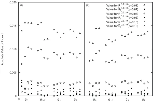
parameters (i) and (ii), design matrices (I)–(IV), and significance level ε = 0.01, 0.05 and 0.10. Fig.2 and Fig.3 show the absolute values of index I when the test statistics are R0.0,1.0 and R1.0,1.0 in the same models and situations as those in the explanation of Fig.1, respectively.
From Fig.1 and Fig.2, we find that the performance of transformed statis-tics ˜R0.2,0.2I and ˜R0.0,1.0I is better than that of original statistics R0.2,0.2 and
R0.0,1.0, respectively, when the models are given by the link functions g0 (com-plementary log-log model), g1/2, g1 (logistic regression model) and gP (probit
model) for the two true parameters, all design matrix cases, and sample design
n∗ = 20. From Fig.3, we find that the performance of transformed statistic ˜
R1.0,1.0I is better than that of original statistic R1.0,1.0when the true parameter is type (i). However, when the true parameter is type (ii), the performance of the transformed statistic is not better than that of the original statistic.
Consequently, from Figs.1–3 and other simulation results, we conclude as follows. The performance of ˜Ra,bI (0 < a ≤ 1, 0 < b ≤ 1) is usually better than that of original statistic Ra,b (0 < a ≤ 1, 0 < b ≤ 1) when the models are given by the link functions g0 (complementary log-log model), g1/2, g1 (logistic regression model) and gP (probit model) under the conditions of the
simulation. However, as shown in Fig.3, when the chi-square approximation of the original statistic performs very well, approximation of the transformed statistic sometimes does not perform better than the original statistic. That is, when the chi-square approximation of the original statistic already performs very well, the transformed statistic sometimes cannot improve the performance of chi-square approximation.
Next, we compare the power of transformed statistics ˜Ra,bI (a̸= 0 or b ̸= 0) with that of the original statistics Ra,b. The power of transformed statistic
˜
R0.0,0.0B for complementary log-log link g0 and probit link gP is shown in Fig.6
and Fig.7 of Taneichi et al. [21]. Against the null model given by (4.1), we consider an alternative model:
(4.2) H1g: πgα∗ = g−1(β1∗+ β2∗xα) + δα (α = 1, . . . , 8),
where
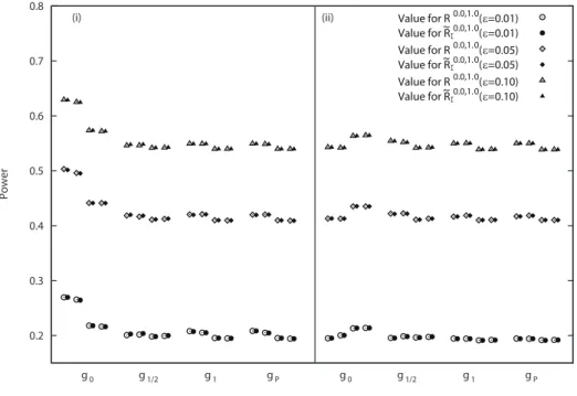
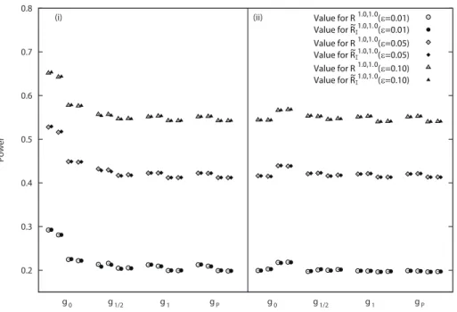
We calculate the simulated average power P against the alternative model (4.2) by using simulated exact critical values of statistics. We investigate the average power for all combinations of the two true parameters (i) and (ii), four design matrices (I)–(IV), and sample design n∗= 20. In the investigation, the number of repetitions is D = 106. Some of the results of the investigations are shown in figures as follows. Figs.4, 5 and 6 show the power of statistics corresponding to the cases in Figs.1, 2 and 3, respectively.
From Figs.4–6 and other simulation results, we conclude that the power against H1g given by (16) of the transformed statistics ˜Ra,bI (0 < a ≤ 1, 0 <
b≤ 1) is not so different from that of the original power divergence statistic
Ra,b in the models based on link functions gc(c = 0, 1/2, 1) and gP.
0 0.002 0.004 0.006 0.008 0.01 0.012 0.014 0.016 0.018 g 0 g 1/2 g 1 g P g 0 g 1/2 g 1 g P (i) (ii) Ab so lute V alue of Index I Value for R0.2,0.2(ε=0.01) Value for R~I0.2,0.2(ε=0.01) Value for R0.2,0.2(ε=0.05) Value for R~I0.2,0.2(ε=0.05) Value for R0.2,0.2(ε=0.10) Value for R~I0.2,0.2(ε=0.10)
Figure 1: Absolute value of index I when the original test statistic is R0.2,0.2and models are given by link functions g0, g1/2, g1and gP for true parameters (i) and (ii) and sample design n∗ =20: ◦, ♢ and △ are the values for R0.2,0.2 when ε =0.01, 0.05 and 0.10, respectively,
and•,♦ and ▲ are the values for ˜R0.2,0.2I when ε =0.01, 0.05 and 0.10, respectively. The 1st
column is for design matrix (I), the 2nd column is for design matrix (II), the 3rd column is for design matrix (III), and the 4th column is for design matrix (IV).
0 0.005 0.010 0.015 0.020 0 g 0 g 1/2 g 1 g P g 0 g 1/2 g 1 g P (i) (ii) Absolut e Value of Index I Value for R0.0,1.0(ε=0.01) Value for R~I0.0,1.0(ε=0.01) Value for R0.0,1.0(ε=0.05) Value for R~I0.0,1.0(ε=0.05) Value for R0.0,1.0(ε=0.10) Value for R~I0.0,1.0(ε=0.10)
Figure 2: Absolute value of index I when the original test statistic is R0.0,1.0.
0 0.001 0.002 0.003 0.004 0.005 0.006 0.007 0.008 g 0 g 1/2 g 1 g P g 0 g 1/2 g 1 g P (i) (ii)
Absolute Value of Index I
Value for R1.0,1.0(ε=0.01) Value for R~I1.0,1.0(ε=0.01) Value for R1.0,1.0(ε=0.05) Value for R~I1.0,1.0(ε=0.05) Value for R1.0,1.0(ε=0.10) Value for R~I1.0,1.0(ε=0.10)
0.2 0.3 0.4 0.5 0.6 0.7 0.8 g 0 g 1/2 g 1 g P g 0 g 1/2 g 1 g P (i) (ii) Power Value for R0.2,0.2(ε=0.01) Value for R~I0.2,0.2(ε=0.01) Value for R0.2,0.2(ε=0.05) Value for R~I0.2,0.2(ε=0.05) Value for R0.2,0.2(ε=0.10) Value for R~I0.2,0.2(ε=0.10)
Figure 4: Simulated average power P against an alternative model (4.2) when the original test statistic is R0.2,0.2 and models are given by link functions g0, g1/2, g1 and gP for true
parameters (i) and (ii) and sample design n∗ = 20: ◦, ♢ and △ are the values for R0.2,0.2 when ε =0.01, 0.05 and 0.10, respectively, and •,♦ and ▲ are the values for ˜R0.2,0.2I when
ε =0.01, 0.05 and 0.10, respectively. The 1st column is for design matrix (I), the 2nd column
is for design matrix (II), the 3rd column is for design matrix (III), and the 4th column is for design matrix (IV).
0.2 0.3 0.4 0.5 0.6 0.7 0.8 g 0 g 1/2 g 1 g P g 0 g 1/2 g 1 g P (i) (ii) Power Value for R0.0,1.0(ε=0.01) Value for R~I0.0,1.0(ε=0.01) Value for R0.0,1.0(ε=0.05) Value for R~I0.0,1.0(ε=0.05) Value for R0.0,1.0(ε=0.10) Value for R~I0.0,1.0(ε=0.10)
Figure 5: Simulated average power P against an alternative model (4.2) when the original test statistic is R0.0,1.0.
0.2 0.3 0.4 0.5 0.6 0.7 0.8 g 0 g 1/2 g 1 g P g 0 g 1/2 g 1 g P (i) (ii) Power Value for R1.0,1.0(ε=0.01) Value for R~I1.0,1.0(ε=0.01) Value for R1.0,1.0(ε=0.05) Value for R~I1.0,1.0(ε=0.05) Value for R1.0,1.0(ε=0.10) Value for R~I1.0,1.0(ε=0.10)
Figure 6: Simulated average power P against an alternative model (4.2) when the original test statistic is R1.0,1.0.
§5. Appendix: Proof of Theorem 2.1 By transformation (2.1), statistic Cϕϕ∗ can be rewitten as
Cϕϕ∗(W ) = 2 N ∑ α=1 nα { ˆ παgϕ∗(W )ϕ ( πgα+ Wα(√nα)−1 ˆ παgϕ∗(W ) ) + ( 1− ˆπαgϕ∗(W ) ) ϕ ( 1− παg − Wα(√nα)−1 1− ˆπgϕα ∗(W ) )} . If we regard hg(w) { 1 +√1 nh g 1(w) + 1 nh g 2(w) + 1 n√nh g 3(w) }
as the continuous density function of W , then we can regard
J1g,ϕϕ∗(x) = ∫ · · · ∫ Uϕϕ∗g (x) hg(w) { 1 +√1 nh g 1(w) + 1 nh g 2(w) + 1 n√nh g 3(w) } dw
as the distribution function of Cϕϕ∗(W ), where
Uϕϕg ∗(x) ={w = (w1, . . . , wN)′ : Cϕϕ∗(w)≤ x}.
So, the characteristic function of Cϕϕ∗(W ) is calculated as
(A1) ψgϕϕ∗(u) = ∫ ∞ −∞· · · ∫ ∞ −∞[exp{iuCϕϕ ∗(w)}] hg(w) × { 1 +√1 nh g 1(w) + 1 nh g 2(w) + 1 n√nh g 3(w) } dw. We can expand Cϕϕ∗(w) as (A2) Cϕϕ∗(w) = τ0g(w)+ 1 √ nτ g,ϕ 1 (w)+ 1 nτ g,ϕϕ∗ 2 (w)+ 1 n√nτ g,ϕϕ∗ 3 (w)+O(n−2), where τ0g(w) = w′(Ω−1− Ξ)w, Ξ = (ξαβ) is a N× N matrix, ξαβ = √ µαG1(α) παg(1− πgα) √ µβG1(β) πβg(1− πβg)σαβ (α, β = 1, . . . , N ), τ1g,ϕ(w) = 3 ∑ a=0 ( N ∑ α=1 Ba+11 (α)C1(α)(w)3−awaα ) , τ2g,ϕϕ∗(w) = 2 ∑ a=0 ( N ∑ α=1 Ba+12 (α)C2(α)ϕ∗ (w)2−aC1(α)(w)2a ) + 1 ∑ a=0 ( N ∑ α=1
Ba+42 (α)C2(α)ϕ∗ (w)1−aC1(α)(w)1+2awα
) + 1 ∑ a=0 ( N ∑ α=1 Ba+62 (α)C2(α)ϕ∗ (w)1−aC1(α)(w)2aw2α ) + N ∑ α=1 B82(α)C1(α)(w)wα3 + N ∑ α=1 B92(α)w4α, B11(α) = µα 3(παg)2(1− παg)2 { 3παg(1− παg)G1(α)G2(α) −(3 + ϕ′′′(1))(1− 2πg α)G1(α)3 } , B21(α) = √ µα (πgα)2(1− παg)2 { −πg α(1− πgα)G2(α) +(2 + ϕ′′′(1))(1− 2πgα)G1(α)2 } ,
B13(α) =− ( 1 + ϕ′′′(1))(1− 2πgα)G1(α) (πgα)2(1− παg)2 , B 1 4(α) = ϕ′′′(1)(1− 2πgα) 3√µα(παg)2(1− παg)2, B12(α) = µαG1(α) 2 πgα(1− πgα), B 2 2(α) = 3B11(α), B32(α) = µα 12(πgα)3(1− παg)3{(π g α)2(1− παg)2(3G2(α)2+ 4G1(α)G3(α)) −6(3 + ϕ′′′(1))πg α(1− πgα)(1− 2παg)G1(α)2G2(α) +(12 + 8ϕ′′′(1) + ϕ(4)(1))(1− 3παg + 3(παg)2)G1(α)4}, B42(α) = 2B21(α), B25(α) = √ µα 3(παg)3(1− παg)3{−(π g α)2(1− παg)2G3(α) +3(2 + ϕ′′′(1))παg(1− παg)(1− 2παg)G1(α)G2(α) −(6 + 6ϕ′′′(1) + ϕ(4)(1))(1− 3πg α+ 3(παg)2)G1(α)3}, B62(α) = B31(α), B72(α) = 1 2(παg)3(1− παg)3{−(1 + ϕ ′′′(1))πg α(1− παg)(1− 2πgα)G2(α) +(2 + 4ϕ′′′(1) + ϕ(4)(1))(1− 3πg α+ 3(πgα)2)G1(α)2}, B82(α) =−(2ϕ ′′′(1) + ϕ(4)(1))(1− 3πg α+ 3(πgα)2)G1(α) 3√µα(πgα)3(1− παg)3 , B92(α) = ϕ (4)(1)(1− 3πg α+ 3(παg)2) 12µα(πgα)3(1− παg)3 , C1(α)(w) = p ∑ m=1 xαm ( p ∑ k=1 κm,kMk(w) ) (α = 1, . . . , N ), C2(α)ϕ∗ (w) = p ∑ m=1 xαm { p ∑ k=1 Mm,k(w)Mk(w) + p ∑ k=1 κm,kSkϕ∗(w) +1 2 p ∑ k1=1 · · · p ∑ k5=1 κm,k3κk1,k4κk2,k5κϕ∗ k3,k4,k5Mk1(w)Mk2(w) } (α = 1, . . . , N ), Mk(w) = N ∑ λ=1 √ µλxλkG1(λ){πλg(1− πλg)}−1wλ (k = 1, . . . , p), Qϕi,j∗(w) = N ∑ λ=1 √ µλxλixλj { −(2 + ϕ∗′′′(1))(1− 2π g λ)G1(λ) 2 (πgλ)2(1− πλg)2 + G2(λ) πλg(1− πλg) } wλ (i, j = 1, . . . , p),
κϕi,j,k∗ = N ∑ λ=1 µλxλixλjxλk { (3 + ϕ∗′′′(1))(1− 2π g λ)G1(λ) 3 (πgλ)2(1− πλg)2 −3Gπ1(λ)G2(λ)g λ(1− π g λ) } (i, j, k = 1, . . . , p), Skϕ∗(w) = 1 2{1 + ϕ ∗′′′ (1)} N ∑ λ=1 xλk (1− 2πgλ)G1(λ) (πλg)2(1− πg λ)2 w2λ (k = 1, . . . , p), Gi(α) = u(i)(x′αβ) (α = 1, . . . , N, i = 1, 2, 3),
Qϕ∗(w) = (Qϕi,j∗(w)) is a p× p matrix, Mi,j(w) is the (i, j)-element of matrix
K−1Qϕ∗(w)K−1, Ω is defined by (2.3), σαβ and K−1 = (κi,j) are defined in
Theorem 2.1, and τ3g,ϕϕ∗(w) is a homogeneous polynomial of degree 5 with respect to variables w1, . . . , wN. Then, from (2.2), (A1) and (A2), we obtain
(A3) ψϕϕg ∗(u) = (1− 2iu)−(N−p)/2
× ∫ ∞ −∞· · · ∫ ∞ −∞(2π) −N/2|Λ|−1/2{exp(−1 2w ′Λ−1w)} × { 1 +√1 nD1(w) + 1 nD2(w) + 1 n√nD3(w) } dw +O(n−2), where Λ = (1− 2iu)−1(Ω− 2iuΩΞΩ),
D1(w) = hg1(w) + (iu)τ1g,ϕ(w), D2(w) = hg2(w) + (iu)τ g,ϕ 1 (w)h g 1(w) + (iu)τ g,ϕϕ∗ 2 (w) + 1 2(iu) 2{τg,ϕ 1 (w) }2 ,
and degrees of all terms of polynomial D3(w) are odd. Therefore, by carrying out the integration of (A3), the characteristic function ψϕϕg ∗(u) is expanded as
(A4) ψgϕϕ∗(u) = (1− 2iu)−(N−p)/2
1 + 1 n 3 ∑ j=0 (1− 2iu)−jvjg,ϕϕ∗+ O(n−2) . By inverting (A4), we obtain (2.4). We have completed the proof of Theorem 2.1.
Acknowledgments
This research is partially supported by the Grants-in-aid for Scientific Research of Japan Society for the Promotion of Science (C) 24540133.
References
[1] Aranda-Ordaz, F. J. (1981). On two families of transformations to additivity for binary response data, Biometrika, 68, 357–363.
[2] Barndorff-Nielsen, O. E. and Cox, D. R. (1984). Bartlett adjustments to the likelihood ratio statistic and the distribution of maximum likelihood estimator,
J. R. Statist. Soc. B, 46, 483–495.
[3] Barndorff-Nielsen, O. E. and Hall, P. (1988). On the level-error after Bartlett adjustment of the likelihood ratio statistic, Biometrika, 75, 374–378.
[4] Cressie, N. and Read, T. R. C. (1984). Multinomial goodness-of-fit tests, J. R.
Statist. Soc. B, 46, 440–464.
[5] Fujikoshi, Y. (2000). Transformations with improved chi-squared approxima-tions, J. Multivariate Anal., 72, 249–263.
[6] Kakizawa, Y. (1996). Higher order monotone Bartlett-type adjustment for some multivariate test statistics, Biometrika, 83, 923–927.
[7] Kullback, S. (1959). Information Theory and statistics, New York Wiley. [8] Lawley, D. N. (1956). A general method for approximating to the distribution of
the likelihood ratio criteria, Biometrika, 43, 295–303.
[9] Men´endez, M. L., Pardo, J. A., Pardo, L. and Pardo, M. C. (1997). Asymp-totic approximations for the distributions of the (h, ϕ)-divergence goodness-of-fit statistics: application to Renyi’s statistic, Kybernetes, 26(4), 442–452.
[10] Nelder, J. A. and Wedderburn, R. W. M. (1972). Generalized linear models, J.
R. Statist. Soc. A, 135, 370–384.
[11] Pardo, L. (2006). Statistical inference based on divergence measures, Chapman & Hall/CRC.
[12] Pardo, J. A. and Pardo, M. C. (2008). Minimum ϕ-divergence estimator and
ϕ-divergence statistics in generalized linear models with binary data, Methodol. Comput. Appl. Probab., 10, 357–379.
[13] Read, T. R. C. (1984). Closer asymptotic approximations for the distributions of the power divergence goodness-of-fit statistics, Ann. Inst. Statist. Math., 36, 59–69.
[14] Read, T. R. C. and Cressie, N. A. C. (1988). Goodness-of-fit statistics for discrete
multivariate data, Springer.
[15] Sekiya, Y. and Taneichi, N. (2004). Improvement of approximations for the dis-tributions of multinomial goodness-of-fit statistics under nonlocal alternatives,
[16] Siotani, M. and Fujikoshi Y. (1984). Asymptotic approximations for the distribu-tions of multinomial goodness-of-fit statistics, Hiroshima Math. J., 14, 115–124. [17] Taneichi, N., Sekiya, Y. and Suzukawa, A. (2001). An asymptotic approximation for the distribution of ϕ-divergence multinomial goodness-of-fit statistic under local alternatives, J. Japan Statist. Soc., 31(2), 207–224.
[18] Taneichi, N., Sekiya, Y. and Suzukawa, A. (2002). Asymptotic approximations for the distributions of the multinomial goodness-of-fit statistics under local al-ternatives, J. Multivariate Anal., 81, 335–359.
[19] Taneichi, N. and Sekiya, Y. (2007). Improved transformed statistics for the test of independence in r×s contingency tables, J. Multivariate Anal., 98, 1630–1657. [20] Taneichi, N., Sekiya, Y. and Toyama, J. (2011). Improved transformed deviance statistic for testing a logistic regression model, J. Multivariate Anal., 102, 1263– 1279.
[21] Taneichi, N., Sekiya, Y. and Toyama, J. (2014). Transformed goodness-of-fit statistics for a generalized linear model of binary data, J. Multivariate Anal.,
123, 311–329.
[22] Yanagihara, H. (1998). Transformations for improving normal and chi-squared approximations, Master’s thesis, Hiroshima University, (in Japanese).
[23] Yarnold, J. K. (1972). Asymptotic approximations for the probability that a sum of lattice random vectors lies in a convex set, Ann. Math. Statist., 43, 1566–1580.
Nobuhiro Taneichi
Department of Mathematics and Computer Science,
Graduate School of Science and Engineering, Kagoshima University 1-21-35 Korimoto, Kagoshima 890-0065, Japan
E-mail : [email protected]
Yuri Sekiya
Kushiro Campus, Hokkaido University of Education Kushiro 085-8580, Japan
E-mail : [email protected]
Jun Toyama
The Institute for the Practical Application of Mathematics Sapporo 063-0001, Japan