Bottom-Left 安定点の効率的な列挙法とその応用 (最適化モデルとアルゴリズムの新展開)

(1)

Bottom-Left

安定点の効率的な列挙法とその応用

名古屋大学大学院工学研究科今堀慎治 (Shinji Imahori) Graduate School of Engineering,

Nagoya University

名古屋大学大学院情報科学研究科簡干耀 (Yuyao Chien)

田中勇真(Yuma Tanaka)

柳浦睦憲 (Mutsunori Yagiura)

Graduate School ofInformation Science,

Nagoya University 概要: 本稿では，既に配置された長方形の集合と

1

つの未配置の長方形が与えられたとき，未配置長方形のBottom-Left 安定点を全て列挙する問題を考える．提案アルゴリズムは，配置された長方形の数を $n$, 未配置の長方形の Bottom-Left安定点の数を $K$

とすると，

$O((n+K)\log n)$_時間で全ての Bottom-Left安定点を列挙する．提案アルゴリズムの特徴の一つに，既配置長方形が Bottom-Left安定でない場合や，既配置長方形間に重なりがある場合にも適用可能であることが挙げられる．計算量の理論的な解析と，数値実験による評価を通して，提案アルゴリズムの有効性を検証する． 1 Introduction

Rectangle packing is animportant problem with applications in steel, wood, glass, paper and

many other industries. There are a number of variants ofthe problem with different objectives and constraints, but the essential task is to place a given set of rectangles in

a

given larger

area

without overlap so that the wasted space in the resulting layout is minimized. (See [14] for atypology of cutting and packing problems.) Almost all variants of the problem

are

known

to be NP-hard, and many heuristic algorithms have been proposed in the literature. One of

the typical frameworks of existing heuristic algorithms is the

_bottom-left

strategy, which places

rectangles one by one at

_bottom-left

stable positions [1, 9, 12]. A fundamental problem to be solved for executing these algorithms is to enumerate all bottom-left stable positions (or to find

a bottom-left stable position with some properties) for a set of already placed rectangles and

one new rectangle to be placed next.

Bottom-left stable positions are defined for a given area (in this paper, we assume the shape

of the given areaisrectangular), aset of rectangles placed in the area, and one newrectangle. A

bottom-left stable position is

a

point in the

area

where the

new

rectangle

can

be placed without overlap with already placed rectangles and the new rectangle cannot

move

to the bottom

or

to

theleft. We note that there are manybottom-left stable positions ingeneral and thelowest one

(ifthere are ties, the leftmost one among the lowest) is called the

_bottom-left

position. We also

define

_bottom-left

stabilityfor a layout; ifthere is no overlap amongrectangles and no rectangle

(2)

Some constructiveheuristic algorithms for the rectangle packing problem place rectangles at a

bottom-left stableposition [1, 3, 7, 9, 12], andhence anylayoutsconstructed by these algorithms

(including intermediate layouts) satisfy bottom-left stability. For layouts with bottom-left

sta-bility, Chazelle [4] showed that the number of bottom-left stable positions for anewrectangle is at most$n+1$ when the numberof placed rectangles is$n$ and proposed

an

algorithm to enumerate

all the bottom-left stable positions in linear time.

Another

common

framework of heuristic algorithms for the rectangle packing problem is

im-provement method, which places all the rectangles in the given

area

without overlap and itera-tively improves the layout by

some

operations. This kind of algorithms often place

a

rectangle at

a bottom-leftstable position, but in this case, theymayneedto solve the problem of finding such

aposition in alayout without

_bottom-left

stability. Forthis case, Healy et al. [6] showed that the number ofbottom-leftstable positions for

a new

rectangle is $O(n)$ when$n$ rectangles are placed

in the area without overlap, and they proposed an $O(n\log n)$ time algorithm to enumerate all

the bottom-leftstable positions.

For

some

packing problems including the two-dimensional irregular packing problem, algo-rithms with compaction and sepamtion opemtions

were

proposed [2, 5, 8, 11, 13]. These

algo-rithms generate layouts with overlap during their execution. However, efficient algorithms to

enumerate bottom-left stable positions in layouts with overlap have not been proposed yet.

In this paper,

we

consider the problem of enumerating bottom-left stable positions for a

new

rectangle within agiven layout that maynot satisfy bottom-left stabilityand mayhave overlap

between rectangles. We propose

an

enumeration algorithm that runs in $O((n+K)\log n)$ time,

where$n$ is the number of placed rectangles and$K$ is the number ofbottom-leftstable positions.

Our algorithm enumerates bottom-left stable positions from bottom to top (from left to right

for positions with same y-coordinates), and hence it outputs the bottom-left position first in

$O(n\log n)$ time.

The bottom-left strategy can naturally be generalized to the three-dimensional

case.

An

important consequence of the algorithm proposed in this paper is that it

can

be utilized to design an efficient algorithm to execute such a bottom-left algorithm for the three-dimensional

packing problem. Kawashima et al. [10] showed that the time complexity

was

improved from

the previous best-known $O(n^{5})$ to $O(n^{3}\log n)$. In their proof, our algorithm is used

as

a

core

part of the algorithm, and the applicability of

our

algorithm to the

case

withrectangles having

overlap is crucial, i.e., existing algorithms such

as

those proposed in [4, 6] cannot be used for

this purpose.

2 Problem description

We are given aset of$n$ rectangles$I=\{1,2, \ldots, n\}$ and one large rectangular area, also called the container. The containerhas its width and height $(W, H)$ anditsbottom left point is placed at (0,0) in the plane. Each rectangle $i\in I$ has its width and height $(w_{i}, h_{i})$, and is placed

orthogonally in the plane. Let $(x_{i}, y_{i})$ be the coordinate of the bottom left point of rectangle $i$

.

We note that the given rectangles may protrudefrom the container and may have overlap each other. We

are

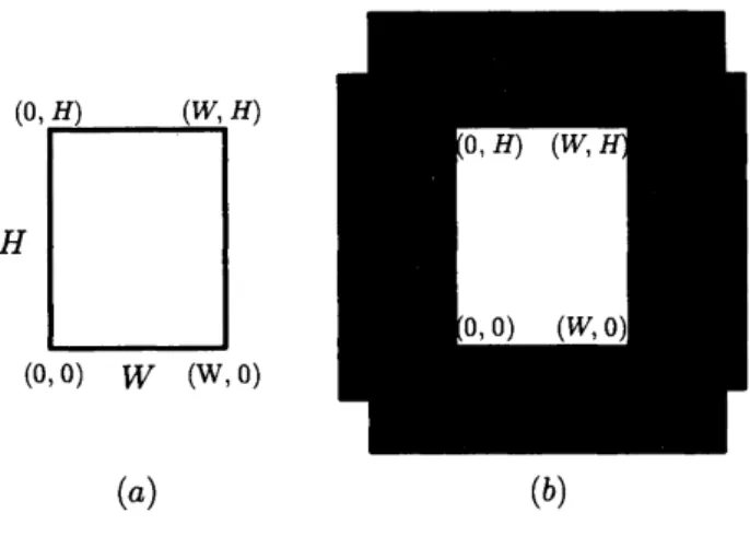
also givenone new rectangle$j\not\in I$ withsize $(w_{j}, h_{j})$ that has not beenplaced yet.

(3)

(0, 司口 $(W, H)$ $(0, H)$ 口 $(W, H)$

$(0,0)$ $(w, 0)$ $(0,0)$ $(w, 0)$

$(a)$ $(b)$

Figure 1: Bottom-left stable positions.

See Figure 1 (a) for

an

example of bottom-left stable positions; black points in this figure denote

bottom-left stable positions for rectangle$j$. Let $K$ be the number ofbottom-left stable positions

for agiven layout and

one

new rectangle. It is known that $K=O(n^{2})$ and $K$

can

be $\Theta(n^{2})$ for

some cases (see Figure 1(b) for an example).

3 Algorithms

In this section, we propose algorithms to enumerate bottom-left stable positions. We first

introduce

_no-fit

polygon, which is often used in packing algorithms to check overlap efficiently.

In Section 3.2, we give a technique to compute for each point $p$ in the plane the number of

no-fit polygons containing $p$ by using sweep line. In Section 3.3, we propose an algorithm for

enumerating bottom-left stable positions. We estimate the computational complexity of

our

algorithms in Section 3.4.

Instead of considering the constraint that requires a new rectangle to be placed in the

con-tainer, we use a set of four sufficiently large virtual rectangles $C=\{c_{1}, c_{r}, c_{t}, c_{b}\}$ that satisfies

the following condition: Rectangle $j$ does not have overlap with rectangles $i’\in I\cup C$ if and

only ifit is placed in the container without overlap with rectangles$i\in I$. We call these virtual

rectangles container rectangles;

see

Figure 2 for an example of container rectangles. We denote

$I’=I\cup C$_; _then _{$|I’|=|I|+4$} _holds.

3.1 No-fit polygon

No-fit

polygon (NFP) is a geometric technique to check overlap of two polygons in

two-dimensional space. It is defined for an ordered pair of two polygons $i$ and $j$, where the position

of polygon $i$ is fixed and polygon _$j$

can

be moved. $NFP(i,j)$ denotes positions of polygon

$j$

having intersection with polygon $i$. In this paper, we treat only the situation that both of two

polygons $i$ and _$j$ are rectangles, and hence it is easy to compute $NFP(i, j)$. Let rectangle $i$ be

placed at $(x_{i}, y_{i})$ and rectangle$j$ be the new rectangle. Then $NFP(i, j)$ is defined as follows:

(4)

$(0, H)$ $(W, H)$

$(0,0)$ $W$ $(W, 0)$

$(a)$ $(b)$

Figure 2: (a) The given area, (b) Container rectangles to represent the

area.

We also definethe overlap number $B(x, y)$ ofno-fit polygons at point $(x, y)$

as

follows:

$B(x, y)=|\{i\in I’|(x, y)\in NFP(i,j)\}|$

.

By using this overlap number, we can characterize bottom-left stable positions

as

follows:

$(x, y)$ is a bottom-left stable position $\Leftrightarrow$

$B(x, y)=0$ A$B(x-\epsilon, y)>0\wedge B(x, y-\epsilon)>0$,

where $\epsilon$ is any sufficiently small positive number. In the next section, we will describe how to

compute overlap number ofno-fit polygons.

3.2 Compute overlap numbers

The algorithm first computes all no-fit polygons $NFP(i,j)$ of rectangle $j$ relative to placed

and container rectangles $i\in I’$

.

Inorder to compute overlap numbers (ofno-fit polygons) in the

given

area

efficiently, the algorithm

uses

a sweep line parallel to the x-axis and

moves

it from bottom to top.

Let $N_{t}$ (resp., $N_{b}$) be the set of all the top (resp., bottom) edges of no-fit polygons and

$N_{tb}=N_{t}\cup N_{b}$. The overlap numbers

on

the sweep line will be changed only when the sweep line encounters a member of $N_{tb}$, and changes occur only in the interval between the left edge

and right edge of the no-fit polygon encountered by the sweep line.

Let $N_{1}$ (resp., $N_{r}$) be the set of all the left (resp., right) edges of no-fit polygons and $N_{1r}=$

$N_{1}\cup N_{r}$. Because there are $n$ placed rectangles and four container rectangles, $|N_{t}|=|N_{b}|=$

$|N_{1}|=|N_{r}|=n+4$ and $|N_{tb}|=|N_{1r}|=2n+8$ hold. The elements in $N_{1r}$

are

sorted in

nondecreasingorder of thex-coordinates of the elements, where ties

are

broken by putting

more

priority to elements in $N_{r}$

.

This tie-breaking rule is important, because if two no-fit polygons

have theirleft and right boundaries at thesame x-coordinate, the newrectangle$j$

can

beplaced

without overlap at the intersection point of boundaries ofthe two no-fit polygons. Let $x_{1r}^{(k)}$ be

the x-coordinate ofthe kth element in the sorted list of$N_{1r}$, and define intervals

$S_{k}=[x_{1r}^{(k)}, x_{1r}^{(k+1)}]$, $k=1,2,$

(5)

on

the sweep line.

The algorithm maintains the overlap number for each interval $S_{k}$ during the computation.

Initially, the sweep line is at

a

sufficiently low position, and it overlaps with

no

NFP. At this

moment, the overlap number ofevery interval $S_{k}$ is zero.

Wenowconsider themoment when thesweeplineencounters amember in $N_{tb}$. Let $NFP(i, j)$

be the rectanglewhose top orbottom edge is encountered bythesweepline, and

assume

that the left (resp., right) edge of$NFP(i, j)$ is the lth (resp., $(r+1)$st) element inthe sorted list of$N_{1r}$. In

this situation, we should change the overlap numbers for intervals $S_{l},$$S_{l+1},$ $\ldots,$

$S_{r}$. To be

more

precise, we should increase (resp., decrease) their overlap numbers by one if the encountered

edge is a member of $N_{b}$ (resp., $N_{t}$). To update overlap numbers on the sweep line efficiently,

we use a complete binary tree whose leaves represent intervals $S_{1},$ $S_{2},$

$\ldots,$$S_{2n+7}$. Here, the kth

leaf from the left corresponds to the interval $S_{k}$, and the

name

of this leaf is $k$

.

We note that

$2n+7$ is not

a

power of two for any $n$, and there

are

remaining leaves on the right side of the

leaf corresponding to interval $S_{2n+7}$. Such remaining leaves are called dummy leaves. Weuse a complete binary treewiththe minimum numberofdummy leaves. Then the number ofdummy

leaves is less than $2n+7$ and the height of this tree is $O(\log n)$. Every node of this tree stores valuesPself, _Pmin andPmax, whose role will be explained later.

For two nodes $u$ and $v$ of the tree, let PATH$(u, v)$ be the set of nodes in the path from

$u$ to $v$ including $u$ and $v$ themselves. Let $g(k)$ be the overlap number for interval $S_{k}$ of the

sweep line. (To be more precise, $g(k)$ is the overlap number of all points in $S_{k}$ except the

left (resp., right) boundary of $S_{k}$ if it corresponds to the left (resp., right) boundary of an

NFP. Thus we need to treat the boundaries carefully considering that each NFP is an open set. When the value of $y$ is fixed to the height of the current sweep line, the function $B(x, y)$

is a lower semicontinuous piecewise linear function consisting of horizontal line segments with

heights $g(1),$ $g(2),$_$\ldots,$$g(2n+7)$ _{aligned in this}_orderfrom left to right.) Forevery dummyleaf$u$,

we set $g(u)=1$.

The algorithmmaintains the values ofPself for all nodes ofthe tree so that

$\sum_{u\in PATH(k,root)}$Pself$(u)=g(k)$

is satisfied for each leaf $k$, where root is the root node of the binary tree. Then it is possible

to compute the overlap number of an interval in $O(\log n)$ time by using the values of_Pself in the path from the corresponding leaf to the root node. We also define the values ofPmin(v) and Pmax(v) for each node $v$ of the complete binary tree as follows:

Pmin$($v$)$ $=$ $\min$ $\sum$ _Pself$(u)$, (1) $k\in Q(v)$

$u\in PATH(k,v)$

Pmax$(v)=$ $\max$ $\sum$ _Pself$(u)$, (2)

$k\in Q(v)$

$u\in PATH(k,v)$

where $Q(v)$ is the set of all leaf nodes in the subtree rooted at the node $v$. By using the value

of $p_{\min}(v)$ (resp., $p_{\max}(v)$) and the values of $p_{self}(u)$ for nodes $u$ in the path from the parent

(6)

equal to

zero

(resp., positive) exist in $Q(v)$

.

Let $u$ and $u’$ be the children of node $v$ and

assume

that the values ofPmin$(u)$ and_Pmin$(u’)$

are

known. In this situation, the valueof_Pmin(v)

can

be computed in constant time by

Pmin$(v)=p_{self}(v)+ \min$

{

$p_{\min}(u)$,_Pmin$(u’)$

}.

(3) The value of_Pmax(v) can be computed similarly.

We

now

explainthe algorithm tokeepthe values ofPself,$p_{\min}$andPmax appropriately. Consider

the moment when the sweep line encounters a member in $N_{tb}$

.

Let $NFP(i, j)$ be the rectangle

whose top or bottom edge is encountered by the sweep line, and let the left (resp., right) edge of $NFP(i,j)$ be the lth (resp., $(r+1)$st) element in the sorted list of $N_{1r}$. Here

we

assume

for

simplicitythat the encountered edge is

a

bottom edge of the NFP. The

case

when

a

top edge is

encountered issimilar; instead ofincreasingthe valuesby one, the algorithm decreases the values

by

one.

The algorithm first finds the leaves $l$ and_$r$ that correspond to the lth and rth intervals

and increases the values ofPself,_Pmin andPmax oftheseleafnodes by

one.

It then traverses nodes

in the paths from theleaf nodes $l$ and _$r$ to theirleast commonancestor _$v$. Duringthis traversal,

whenever a node in the path from $l$ (resp., r) to _$v$ is reached from its left (resp., right) child,

the algorithm increases the values of$p_{self}$,Pmin and Pmax of the right (resp., left) child by

one.

It also updates$p_{\min}$ (by using (3)) andPmax for nodes in the paths from $l$ and$r$ to$v$

so

that the

conditions (1) and (2) are satisfied. Finally, the algorithm updates the valuesofPmin andPmax

for all nodes in the path from $v$ to the root node of the tree. The details of this procedure is

summarized

as

Algorithm UPDATEVALUES$(\lambda, l, r)$.

Algorithm UPDATEVALUES$(\lambda, l, r)$

Input: An index $\lambda(\lambda=1$ when the sweep line encounters a bottom edge of NFP; $\lambda=-1$

when the sweep line encounters a top edge ofNFP), two leaves $l$ and _$r$ corresponding to

the leftmost and rightmost intervals and current values of$p_{self}$, Pmin and$p_{\max}$

.

Task: Update the values of$p_{self}$, Pmin and$p_{\max}$.

Step 1: Increasethe valuesof_Pself$(l)$,_Pmin$(l)$,_Pmax$(l),$ $p_{self}(r)$,_Pmin$(r),p_{\max}(r)$ by $\lambda$ (thismeans

that if$\lambda=-1$, these values are actually decreased by one).

Step 2: Let $l_{prev}$ $:=l$ and $r_{prev}$ $:=r$, andthen let $l$ be the parent of$l$ and $r$ be the parent of$r$.

If $l\neq r$, proceed to Step 3; otherwise go to Step 4.

Step 3: If the right (resp., left) child$u$of$l$ (resp., r) is different from

$l_{prev}$ (resp., $r_{prev}$), increase

the values ofPself$(u)$,_Pmin$(u)$and$p_{\max}(u)$ by$\lambda$

.

Let

Pmin$(l)$ $:=p_{self}(l)+ \min$

{

$p_{\min}(u)$,_Pmin$(u’)$

},

where $u$ and $u’$ are the children of node $l$. Update the values of_{$p_{\max}(l)$},

Pmin$(r),p_{\max}(r)$ similarly. Return to Step 2,

Step 4: For each node $v$ in the path from $l(=r)$ to the root and the children $u$ and $u’$ of$v$, let

(7)

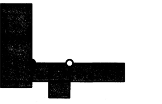
Figure 3: No-fit polygons whose top edges have the same y-coordinate.

3.3 Enumerate bottom-left stable positions

We explain our algorithm that enumerates bottom-left stable positions. Observe that, while

the sweep line parallel to the x-axis is moved from bottom to top, the overlap numbers of

no-fit polygons for intervals in the sweep line decrease only if the top edge of

a

no-fit polygon is encountered. This

means

that bottom-left stable positions

can

be found only in this case,

because apoint $(x, y)$ canbe abottom-left stableposition onlyif_{$B(x, y)=0$} and$B(x, y-\epsilon)>0$

for any sufficiently small positive $\epsilon$. For this reason, when the sweepline encounters thebottom

edge ofano-fit polygon, the algorithmjust updates the overlap numbers according to the rule described in Section 3.2. On the other hand, when the sweep line encounters the top edge of

a no-fit polygon, the algorithm updates the overlap numbers and outputs bottom-left stable positions onthe sweep line if such positions exist. To manage these events, the elements in $N_{tb}$

are sorted in nondecreasing order of they-coordinates of theelements, where ties are broken by putting more priority to elements in$N_{t}$. If the top edges ofsome no-fit polygons have the same

y-coordinate, we put more priority to those elements that correspond to no-fit polygons whose

left edge have smaller x-coordinates.

At any point $(x, y)$ such that the overlap number $B(x, y)$ is equal to zero, we can place

rectangle $j$ without overlap. Moreover, if the overlap number becomes zero when the top edge

of a no-fit polygon is encountered by the sweep line, then $B(x, y-\epsilon)>0$ for any sufficiently

small $\epsilon>0$, i.e., rectangle $j$ cannot

move

downward from the point. Furthermore, ifthe point

$(x, y)$ is at the left boundary ofan _interval $S_{k}$ and its left adjacent interval $S_{k-1}$ has a positive

overlap number, then $B(x-\epsilon, y)>0$ for any sufficiently small $\epsilon>0$, i.e., rectangle$j$ cannot

move to the left, provided that all the top edges of no-fit polygons whose y-coordinates

are

$y$

have already been encountered by the sweep line. Such a point $(x, y)$ is

a

bottom-left stable

position, and our algorithm enumerates all such points. We note that, if there are some no-fit

polygons whose top edges have thesame y-coordinate, all such top edges should leave thesweep line together. Otherwise, the algorithm may output positions from which rectangle $j$ can move

to the left as depicted in Figure 3; when rectangle $i$’ leaves the sweep line, black and white

pointsmay be output asbottom-left stable positions. The details ofouralgorithm to enumerate

(8)

Algorithm ENUMERATEBL$(j, I)$

Input: Placed rectangles $i\in I$ inthe given

area

and

one new

rectangle $j\not\in I$.

Output: All bottom-left stable positions for rectangle $j$.

Step 1: Compute all no-fitpolygonsof rectangle$j$relativeto allplacedand container rectangles

$i\in I’$

.

Sortleft and right edges $N_{1r}$ $:=N_{1}\cup N_{r}$ofno-fit polygonswith the rule described in

Section 3.2. Createtheminimumcomplete binary tree with at least$2n+7$leaves. Initialize

the values$p_{self}(u)$ $:=0$, _Pmin$(u)$ $:=0$ and_Pmax$(u)$ $:=0$ for all leaf nodes $u$corresponding to

intervals $S_{1}$ to _{$S_{2n+7}$}, and initialize thevalues_{$p_{self}(u)$} $:=1$,

Pmin$(u)$ $:=1$ and$p_{\max}(u)$ $:=1$

for all dummy leaves$u$

.

For all internal nodes $u$, set $p_{self}(u)$ $:=0$ andcompute the values

of_Pmin$(u)$ and$p_{\max}(u)$

.

Sort

top andbottomedges $N_{tb}$ $:=N_{t}\cup N_{b}$ of no-fit polygonswith

the rule described in Section 3.3.

Step 2: Choose the first element $e\in N_{tb}$ and let $N_{tb}$ $:=N_{tb}\backslash \{e\}$

.

If the y-coordinate of

element $e$ is greater than H–hj, then stop.

Step 3: Let $i\in I’$ be the no-fit polygon having the element $e$

as

its top

or

bottom edge, and

assume

that its left (resp., right) edge is the lth (resp., $(r+1)$st) element in $N_{1r}$. If$e\in N_{t}$ (resp., $N_{b}$), then set $\lambda$ $:=-1$ (resp., $\lambda$ $:=1$). Call algorithm UPDATEVALUES

$(\lambda, l, r)$

.

Step 4: If$e\in N_{b}$, return to Step 2; otherwise $(i.e., e\in N_{t})$, set $\alpha$ $:=l$ and $\beta$ $:=r$.

Step 5: Let $e$‘ be the first element in $N_{tb}$

.

If$e$ and $e$‘ have the

same

y-coordinate and $e’\in N_{t}$,

go to Step 6; otherwise go to Step 7.

Step 6: Let $i’\in I’$ bethe no-fit polygon having the element $e’$

as

itstop edge, and assumethat

its left (resp., right) edge is the

l’th

(resp., $(r’+1)$st) element in $N_{1r}$

.

If $l’>\beta$ holds, go

to Step 7; otherwise let $N_{tb}:=N_{tb}\backslash \{e’\}$ and call algorithm UPDATEVALUES$(-1, l^{f}, r’)$. If $r’>\beta$ holds, set $\beta$ $:=r’$

.

Return to Step 5.

Step 7: If the overlap number of interval $S_{\alpha}$ is positive, go to Step 8. Ifthe overlap number of

interval $S_{\alpha}$ is equal to $0$ and that ofinterval $S_{\alpha-1}$ is positive, then output a bottom-left

stable position $(x, y)$, where $x=x_{1r}^{(\alpha)}$ and

$y$ is the y-coordinate ofthe current sweep line.

Go to Step 9.

Step 8: Byusingthe values ofPmin, find the leftmost interval$S_{\gamma}$ that satisfies$\gamma>\alpha$ andwhose

overlapnumber is equalto$0$. If$\gamma>\beta$or sucha$\gamma$is notfound, return to Step 2; otherwise,

output abottom-left stable position $(x, y)$, where $x=x_{1r}^{(\gamma)}$ and

$y$is they-coordinateofthe

current sweep line. Let $\alpha$ _$:=\gamma$ and go to Step 9.

Step 9: By usingthe valuesofPmax, findtheleftmost interval$S_{\gamma}$ that satisfies $\gamma>\alpha$and whose

overlap number is positive. If$\gamma\geq\beta$ or such a $\gamma$ is not found, return to Step 2; otherwise,

let $\alpha$

$:=\gamma$ and go to Step 8.

The overlap number of every dummy leaf is initialized to one and is not changed during the execution of the algorithm, and hence the dummy leaf nodes have

no

influence

on

the output of

(9)

this algorithm. By executing this algorithm, allthe bottom-left stable positions are enumerated from bottom to top (from left to right for positions with same y-coordinates).

In Step 8, $\gamma$ is found

as

follows. The algorithm first climbs the binary tree from the leaf$\alpha$,

and whenever a node $v$ is reached from its left child, it checks whether the subtree rooted at

the right child $u$ of$v$ has a leafwhose overlap number is zero. When the first node $u$ having

such aleafis found, the algorithm goes down the tree from the $u$, choosing the left-most child

including such aleaf. In Step 9, the leaf$\gamma$ is found similarly.

3.4 Computational complexity

We estimate the time complexity of our algorithms described in Sections 3.2 and 3.3.

Al-gorithm UPDATEVALUES$(\lambda, l, r)$ runs in $O(\log n)$ time since the height of the complete binary tree is $O(\log n)$

.

Algorithm ENUMERATEBL$(j, I)$ calls algorithm UPDATEVALUES$(\lambda, l, r)$

as a

subroutine at most $2n+8$ times in Steps 3 and 6; then the total timefor this part is $O(n\log n)$.

The time complexity of Step 7 is $O(\log n)$ and it is called at most $n+4$ times. The time com-plexity of Step 8 is $O(\log n)$ because $O(\log n)$ nodes

are

visited during the traversal from $\alpha$ to $\gamma$, and it is possible for each node $u$ to check whether the subtree rooted at the node $u$ has a

leaf node whose overlap number is equal to zero in constant time (this is not hard to see from

the property explained in Section 3.2 just after equation (2)$)$. The timecomplexity of Step 9 is

also $O(\log n)$ for asimilar

reason.

Steps 8 and 9

are

called at most _$n+4+K$ times, where$K$ is

the number of bottom-left stable positions enumerated. Insummary, the total time complexity

of algorithm ENUMERATEBL$(j, I)$ is $O((n+K)\log n)$

.

Furthermore, ifour algorithms are uti-lized for finding the bottom-left position (i.e., the lowest (if there are ties, the leftmost among

ties) bottom-left stable position), algorithm ENUMERATEBL$(j, I)$ can be stopped immediately

when it finds the first bottom-left stable position. In this case, the time complexity to find the

bottom-left position is $O(n\log n)$.

4 Computational results

In this section, we evaluate the proposed algorithms via computational experiments. All the algorithms were coded in $C$ and experiments were conducted on a PC (Intel Xeon _$3GHz,$ _$2MB$

cache, lGB memory). As

a

set of placed rectangles, we used test instances for the rectangle packing problem with 16,32, 64,

. .

., 1048576 rectangles (these instances are obtained electron-ically from http://www.na.cse.nagoya-u.ac.jp$/\sim$imahori/packing/instance.html). The size of

a

new rectangle to be placed next is similar to the placed rectangles.

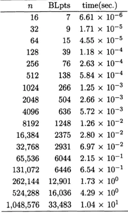
Table 1 shows the computational results. Column $(n$“ shows the number ofrectangles placed

in a rectangular area. The number of bottom-left stable positions enumerated is shown in

column ”BLpts,” and computation time in seconds is reported in column “time(sec.).” We

note that layouts were randomly generated many times (at least 10 times; it depends on the number ofplaced rectangles) and theaveragenumberof bottom-left stable positions andaverage

computation time were reported. From the table, we can observe that the proposed algorithm

enumerates bottom-left stable positions in a short time. It can enumerate all the bottom-left stable positions among hundreds of rectangles within 0.001 seconds, it spends less than 0.1

(10)

Table 1: Performance ofour algorithm. $\frac{nBLptst.ime(sec.)}{167661\cross 10^{-6}}$ 32 9 1.71 $\cross 10^{-5}$ 64 15 4.55 $\cross 10^{-5}$ 128 39 1.18 $\cross 10^{-4}$ 256 76 2.63 $\cross 10^{-4}$

512

138

5.84

$\cross 10^{-4}$

1024

266 1.25

$\cross 10^{-3}$ 2048 504 2.66 $\cross 10^{-3}$ 4096 636 5.72 $\cross 10^{-3}$ 8192 1248 1.26 $\cross 10^{-2}$ 16,384 2375 2.80 $\cross 10^{-2}$ 32,768 2931 6.97 $\cross 10^{-2}$ 65,536 6044 2.15 $\cross 10^{-1}$ 131,072 6446 6.54 $\cross 10^{-1}$ 262,144 12,901 1.73 $\cross 10^{0}$ 524,288 16,036 4.29 $\cross 10^{0}$ 1,048,576 33,483 1.04 $\cross 10^{1}$

seconds for instances with up to 32,768 rectangles, and it takes 10.4 seconds to enumerate all the bottom-left stable positions in layouts with about

one

million rectangles.

5 Conclusions

In this paper, the problem ofenumerating bottom-left stable positions for a given layout of rectangles

was

studied. We proposed an algorithm that enumerates all the bottom-left stable positions in $O((n+K)\log n)$ time, where $n$ is the number of placed rectangles and $K$ is the

number of bottom-left stable positions (i.e., size of the output). Ouralgorithm works for layouts without bottom-left stability and with overlaps. We also evaluated the proposed algorithm via

computational experiments. Even for instances with more than one million placed rectangles,

theproposed algorithm works in ashort computation time.

A direction of future work is to propose faster algorithms: Our algorithm

runs

in $O((n+$

$K)\log n)$ time, but the existence of algorithms that run in $O(n\log n+K)$ is open.

References

[1] Baker, B. S., Coffman, E. G., Rivest, R. L., Orthogonal packings in two dimensions. SIAM

Journal on Computing. 9 (1980) 846-855.

[2] Bennell, J. A., Dowsland, K.A., Hybridising tabu search with optimisation techniques for irregular stockcutting. Management Science. 47 (2001) 1160-1172.

(11)

[3] Burke, E. K., Kendall, G., Whitwell, G., A

new

placement heuristic for the orthogonal stock-cutting problem. Operations Research. 52 (2004) 655-671.

[4] Chazelle, B., The bottom-left bin packing heuristic: an efficient implementation. IEEE Tkansactions on Computers. 32 (1983) 697-707.

[5] Gomes, A. M., Oliveira, J. F., Solving irregular strip packing problems by hybridising

simulated annealing and linear programming. European Journal of Operational Research.

171 (2006)

_811-829.

[6] Healy, P., Creavin, M., Kuusik, A., An optimal algorithm for rectangle placement. Opera-tions Research Letters. 24 (1999) 73-80.

[7] Imahori, S., Yagiura, M., The best-fit heuristic for the rectangular strip packing

prob-lem: an efficient implementation and the worst-case approximation ratio. Computers and Operations Research. 37 (2010) 325-333.

[8] Imamichi, T., Yagiura, M., Nagamochi, H., An iterated local search algorithm based on

nonlinear programming for the irregular strip packing problem. Discrete optimization. 6 (2009) 345-361.

[9] Jakobs, S., On genetic algorithms for the packing of polygons. European Journal of

Oper-ational Research. 88 (1996) I65-181.

[10] Kawashima, H., Tanaka, Y., Imahori, S., Yagiura, M., An efficientimplementation ofa

con-structive algorithm for the three-dimensional packing problem (in Japanese). Proceedings of the 9th Forum on Information Technology 2010 (FIT2010), Issue 1, pp. 31-38.

[11] Li, Z., Milenkovic, V., Compaction and separation algorithms fornon-convex polygons and

their applications. European Journal ofOperational Research. 84 (1995) 539-561.

[12] Liu, D., Teng, H., An improved BL-algorithm for genetic algorithm of the orthogonal packing of rectangles. European Journal of Operational Research. 112 (1999) 413-420.

[13] Umetani, S., Yagiura, M., Imahori, S., Imamichi, T., Nonobe, K., Ibaraki, T., Solving the

irregular strip packing problem via guided local search for overlap minimization.

Interna-tional Transactions in Operational Research. 16 (2009) 661-683.

[14] W\"ascher, G., Haussner, H., Schumann, H., An improved typology of cutting and packing