Optimal Portfolio Selection by CVaR-Based Sharpe Ratio : Sequential Linear Programming Approach(Mathematical Models and Decision Making under Uncertainty)

Optimal

Portfolio

Selection

by

CVaR-Based

Sharpe

Ratio

Sequential Linear Programming Approach

Shan LIN

(

林

杉

)

and

Masamitsu

OHNISHI

(

大西 匡光

)

Graduate School of

Economics,

Osaka

University

(

大阪大学大学院・経済学研究科

)

1

Introduction

We address an optimal portfolio selection problem ofmaximizingso wecall CVaR (Conditional

$\mathrm{V}\mathrm{a}\mathrm{l}\mathrm{u}\mathrm{e}-\mathrm{a}\mathrm{t}-\mathrm{R}\mathrm{i}\mathrm{s}\mathrm{k})$-based Sharpe ratio of portfolio’s return rate, which is defined as the ratio

of the expected

excess

return to CVaR. The Sharpe ratio defined

as

the ratio of expected

excess

return tostandard deviation, the most

common

traditional performancemeasure, takes

standard deviation as a risk measure, however its has beenreceived a lot ofcriticisms. In our CVaR-basedSharpe ratio, thestandarddeviation is replaced withCVaR, which is aremarkable coherent risk

measure

which

overcomes

essential defects ofstandard deviation. Although

our

new performance

measure

is expected to enlarge the applicable

area

of practical investment problems for which the original Sharperatio is not suitable,however, weshould device effective computational methods to solve optimal portfolio selection problems with very large number ofinvestment opportunities.

In order to deal with rather complicated

non-concave

objective function, whichcomes from

the introduction of CVaR,

we

propose the following SLP (Sequential Linear Programming) approach: By introducing a real parameter, we make the

non-concave

maximization problem to a parametric family of

concave

maximization problems. Then, for each of these problems, utilizing the results of Rockafellar and Uryasev (2000),

we

introduce an auxiliary decision

variable

to obtain a tractable

concave

maximization proble1n. Furthermore, if

we

estimate or

approximate required expected values bysamplingmethods orhistoricaldata,

we

can reduce the parametric

concave

maximizationproblems to LP (Linear Programming) problems. Therefore,

our problem could be finally reduced to a sequence of LP problems. Numerical experiments from real Japanesefinancial data are conductedto test our SLP approach.

The

paper

is organized as follows. In Section 2, we introduce downside risk

measures:

$\mathrm{V}\mathrm{a}\mathrm{R}$ and CVaR, in Section 3,

we

make a brief review of parametric approach to fractional

programming. Sample approach will be presented in Section 4. Further, in Section 5 an empirical study is given.

2

VaR and

CVaR

Let $\tilde{r}$denote arandom variable denoting a rate of return on an asset or a portfolio of assets.

Value at Risk $(\mathrm{V}\mathrm{a}\mathrm{R})$ of

$\overline{r}$with confidence level $\beta\in[0,1]$, denoted

negative of $(1-\beta)$-quantile of$\overline{r}.\cdot$

$\mathrm{V}\mathrm{a}\mathrm{R}_{\beta}[\neg r$ _$:=$ $- \inf\{r\in \mathbb{R} : \mathrm{P}(\overline{r}\leq r)\geq 1-\beta\}$

$=$ $\sup\{u\in \mathbb{R} : \mathrm{P}(-\mathrm{r}\geq u)\geq 1-\beta\}$. (1)

ConditionalValue at Risk (CVaR) of $\overline{r}$with confidence level

$\beta\in[0,1]$, denoted $\mathrm{C}\mathrm{V}\mathrm{a}\mathrm{R}_{\beta}[\urcorner r$,

is then defined as follows:

$\mathrm{C}\mathrm{V}\mathrm{a}\mathrm{R}_{\beta}[\neg r:=\frac{1}{1-\beta}\int_{0}^{1-\beta}.\mathrm{V}\mathrm{a}\mathrm{R}_{\alpha}[\hat{r}]\mathrm{d}\alpha.$ (2) It can be shown that

$\mathrm{C}\mathrm{V}\mathrm{a}\mathrm{R}_{\beta}[\neg r=\frac{1}{1-\beta}\mathrm{E}$[$-\overline{r}\cdot-)r-\geq \mathrm{V}\mathrm{a}\mathrm{R}_{\beta}[r\urcorner]-\mathrm{V}\mathrm{a}\mathrm{R}\mathrm{O}[\mathrm{r}]$

{

$\mathrm{P}$(-r

$\geq \mathrm{V}\mathrm{a}\mathrm{R}_{\beta}$[$r\neg)-(1-\beta)$

}

, (3) where $\mathrm{E}[Y;\mathrm{A}]$ denotes the partial expectation of a random variable $Y$ on

an

event $A$; that is

$\mathrm{E}[Y\cdot a]\};=\mathrm{E}[Y1_{A}]$. Although this expression is somewhat complex, if

$\mathrm{P}$$(-\overline{r}\geq \mathrm{V}\mathrm{a}\mathrm{R}_{\beta}[\neg r )=1-\beta$, (4)

then the second term vanishes and it becomes

$\mathrm{C}\mathrm{V}\mathrm{a}\mathrm{R}_{\beta}[\neg r=\frac{1}{1-\beta}\mathrm{E}[-\overline{r},\cdot-\overline{r}\geq \mathrm{V}\mathrm{a}\mathrm{R}_{\beta}[\neg r ]=\mathrm{E}$[$-\neg r-\overline{r}\geq \mathrm{V}\mathrm{a}\mathrm{R}_{\beta}[r\neg]$ (5)

Average Value at Risk (AVaR), Expected Shortfall (ES), Tail Conditional Expectation (TCE), andothersaresimilar concepts, not few researchers preferoneoftheseterms toCVaR, but these become identical when the above condition holds (whose sufficient condition is the continuity of cumulative distribution function (cdf) of$\gamma r$

.

A veryuseful characterization is obtained by Pflug (2000), Uryasev (2000), and Rockafellar

and Uryasev $(2000, 2001)$. Let

us

_introduce

a

_function:

$F_{\beta}(a,\cdot\gamma r$ $:=a+ \frac{1}{1-\beta}\mathrm{E}[(-\tilde{r}-a)^{+}]$, $a\in \mathbb{R}$, (6)

then the following theorem holds (for

a

real number $c\in \mathbb{R}$, ($c \rangle^{+}:=\max\{c, 0\}$ is the positive

part of$c$).

Theorem 1.

(1) $\mathrm{C}\mathrm{V}\mathrm{a}\mathrm{R}\beta[\neg r$ coincides with the minimum of function $F_{\beta}(\cdot;\overline{r})$:

$\mathrm{C}\mathrm{V}\mathrm{a}\mathrm{R}_{\beta}[\neg r’=\min\{F_{\beta}(a,\cdot r\gamma :a\in \mathbb{R}\}$. (7)

(2) The minimum offunction $F_{\beta}(\cdot;\tilde{r})$is attained at when the variable is equal to

$\mathrm{V}\mathrm{a}\mathrm{R}_{\beta}[\neg r$:

$\min\{F_{\beta}(a;\overline{r}) : a\in \mathbb{R}\}=F_{\beta}(\mathrm{V}\mathrm{a}\mathrm{R}_{\beta}[\tilde{r}(x)];r\gamma$ . (8)

(3) $F_{\beta}(a;\tilde{r})$ is convex both in $a\in \mathbb{R}$ and $\overline{r}$

.

$\square$

Now let

us

consider a portfolio optimization of investments in financial assets numbered

$\bullet$ $r-i$, $\mathrm{i}=1$,$\cdots$ ,$n$: the random rate of return on financial asset ;

$\bullet$ $\overline{r}_{i}:=\mathrm{E}[\overline{r_{i}}]$, $\mathrm{i}=1$,$\cdots$ ,$n$: the mean (or expected) rate of return

on

financial asset $\mathrm{i}$; $\bullet$ $x_{i}(\in \mathbb{R})$, $\mathrm{i}=1$,$\cdots$ ,$n$: aportfolio weight, that is, aproportion ofinvestment in financial

asset $\mathrm{i}$;

$\bullet$ $r-.–$ $(\tilde{r}_{1}, \cdots,\overline{r}_{n})^{\mathrm{T}}$: the random vector ofreturn rates on financial assets $\mathrm{i}=1$,$\cdots$ ,$n,\cdot$

$\bullet$ $\overline{r}:=(\overline{r}_{1}, \cdots)$$\overline{r}_{n})^{\mathrm{T}}$: the vector ofmean return rates on financial assets $\mathrm{i}=1$,$\cdots$ ,$n$;

$\bullet$ $x:=$ $(x_{1}, \cdots, x_{n})^{\mathrm{T}}$: the portfolio of investment proportions in financial assets

$\mathrm{i}=$

1,$\cdots$ ,$n$.

Further

we

let

$\mathrm{r}(\mathrm{x})$ _$:=$ $\tilde{r}^{\mathrm{T}}x=\sum_{l=1}^{n}\overline{r_{i}}x_{i)}$. (9)

$\mathrm{r}(\mathrm{x})$ $:= \mathrm{E}[\overline{r}(x)]=\mathrm{E}[\tilde{r}^{\mathrm{T}}x]=\sum_{i=1}^{n}\mathrm{E}[\tilde{r}_{i}]x_{i}=\overline{r}^{\mathrm{T}}x=\sum_{i=1}^{n}\overline{r}:x_{0}$

.

(1)

Theabovetheoremisparticularlyuseful whenwe mustconsider the minimization of$\mathrm{C}_{J}\mathrm{V}\mathrm{a}\mathrm{R}_{\beta}[\overline{r}(x)]$ ofreturn rate $\mathrm{r}(\mathrm{x})$ on portfolio $x$. According to the definition of $\mathrm{C}\mathrm{V}\mathrm{a}\mathrm{R}_{\beta}[\overline{r}(x)]$, for every eval-uation of the objective function at $x\in X$, we must evaluate the values in the order:

(1) $\mathrm{V}\mathrm{a}\mathrm{R}_{\beta}[\overline{r}(x)]$ $\supset$ (2) $\mathrm{C}\mathrm{V}\mathrm{a}\mathrm{R}_{\beta}[\tilde{r}(x)]$, (11) but these are tremendous tasks. The following theorem implies that the evaluation and

mini-mization of $\mathrm{C}\mathrm{V}\mathrm{a}\mathrm{R}_{\beta}[\tilde{r}(x)]$can be done by the simultaneous minimization of function $\Gamma\prec(a;\overline{r}(x))$ with respect to the original decision variable $x\in X$ and

an

auxiliary variable $a\in \mathbb{R}$_.

Theorem 2. (1)

$\min\{\mathrm{C}\mathrm{V}\mathrm{a}\mathrm{E}_{\beta}[\overline{r}(x)] :x\in X\}$$= \min\{F\beta(a;\overline{r}(x)) : a\in \mathbb{R},\cdot x\in X\}$. (12)

(2) For $x^{*}\in X$,

$\min\{\mathrm{C}\mathrm{V}\mathrm{a}\mathrm{R}_{\beta}[\overline{r}(x)] :x\in X\}$$=\mathrm{C}\mathrm{V}\mathrm{a}\mathrm{R}\beta[\overline{r}(x^{*})]$ (13)

ifand only if

$\min\{F_{\beta}(a;\tilde{r}(x)) :a\in \mathbb{R}_{\mathrm{j}}x\in X\}=F_{\beta}(\mathrm{V}\mathrm{a}\mathrm{R}_{\beta}[\tilde{r}(x^{*})];\overline{r}(x^{*}))$ . (14)

(3) $F_{\beta}(a;\tilde{r}(x))$ is

convex

both in$a\in \mathbb{R}$ and $x\in X$

.

$\square$ Accordingly, the original convex program ming problem with $n+1$ decision variables;

$|\mathrm{M}\mathrm{i}\mathrm{n}\mathrm{i}\mathrm{m}\mathrm{i}\mathrm{z}\mathrm{z}\mathrm{e}\mathrm{s}\mathrm{u}\mathrm{b}\mathrm{j}\mathrm{e}\mathrm{c}\mathrm{t}\mathrm{t}\mathrm{o}$ $x\in X\mathrm{C}\mathrm{V}\mathrm{a}\mathrm{R}_{\beta},[\tilde{r}(x)]$ (15)

couldbe reduced to the following

convex

programming problem with $n+1$ decision variables; $|\mathrm{s}\mathrm{u}\mathrm{b}\mathrm{j}\mathrm{e}\mathrm{c}\mathrm{t}\mathrm{t}\mathrm{o}\mathrm{M}\mathrm{i}\mathrm{n}\mathrm{i}\mathrm{m}\mathrm{i}\mathrm{z}\mathrm{z}\mathrm{e}$ $x \in’ Xa\in \mathbb{R}_{j}F_{\beta}(a\cdot\overline{r,}(x)).--a+\frac{1}{1-\beta}\mathrm{E}[(-\tilde{r}(x)-a)^{+}]$ (16)

3

Fractional

Programming

Let

us

consider a fractional programming problem formulated

as

follows: [P] $|\mathrm{s}\mathrm{u}\mathrm{b}\mathrm{j}\mathrm{e}\mathrm{c}\mathrm{t}\mathrm{t}\mathrm{o}\mathrm{M}\mathrm{a}\mathrm{x}\mathrm{i}\mathrm{m}\mathrm{i}\mathrm{z}\mathrm{e}x\in Xh(x).--$

,

$\frac{f(x)}{g(x)}$

(1)

where

$\bullet x=(x_{1}, \cdots, x_{n})^{\mathrm{T}}$:

$\bullet$ $X\subset \mathbb{R}^{n}$: a

convex

and compact constraint set;

$\bullet$ $f$ : $X-arrow \mathbb{R}$: a continuous function on $X$;

$\bullet$ _$g$ : _{$Xarrow \mathbb{R}_{++}:$} a continuous positive-valued function on $X$. $\bullet$ $h$ : $Xarrow \mathbb{R}$: a continuous function

on

$X$

.

If

(A1) $f$: a linear (or, more generally, concave) function on $X$;

(A2) $g$: a convex function on $X$

then

$h:=f/g$ : $Xarrow \mathbb{R}$ : a($\mathrm{n}$ essentially) quasi-concavefunction on $X$ (2)

because, for a (nonnegative) level $z\in \mathbb{R}_{+}$, the level set

$L_{h}(z)$ $:=$ $\{x\in X : h(x)\geq z\}$

$=$ $\{x\in X : f(x)-zg(x)\geq 0\}$ : a

convex

set in $\mathbb{R}^{n}$ (3) which isdue to

f-zg. $Xarrow \mathbb{R}$ :

a concave

function on X. (4)

Now, by introducing areal parameter $z\in \mathbb{R}$, let us consider $[\mathrm{Q}(z)]$ $|\mathrm{s}\mathrm{u}\mathrm{b}\mathrm{j}\mathrm{e}\mathrm{c}\mathrm{t}\mathrm{t}\mathrm{o}\mathrm{M}\mathrm{a}\mathrm{x}\mathrm{i}\mathrm{m}\mathrm{i}\mathrm{z}\mathrm{e}$ $x\in.Xu(x,z)$

, (5)

where, for each $z\in \mathbb{R}$, we define

$u(x;z):=f(x)-zg(x)$ : $Xarrow \mathbb{R}$ (6)

Since, for any $z\in \mathbb{R}$, the function $u(x;z)$ is a continuous function of_{$x\in X$}, and $X\in \mathbb{R}^{n}$ is a

compactset, byWeierstrassTheorem, theproblem $\mathrm{Q}(z)$ has anoptimalsolution, say$x(z)\in X$,

$\mathrm{F}\mathrm{u}\mathrm{r}\mathrm{t}\mathrm{l}\uparrow\circ \mathrm{r}$Let us define theoptimal

value function by

$v(z)$ $:= \max\{u(x;z) : x\in X\}$

$=$ $\max\{f(x)-zg(x) : x\in X\}$ $=$ $\{f(x(z))-zg(x(z))$, $z\in \mathbb{R}$.

Since,for each$x\in X$, $u(x;z)=f(x)-zg(x)$ is amonotonedecreasinglinear function of$z\in \mathbb{R}$,

and $v(z)$ is a function composed of pointwise maximum of such linear $\mathrm{f}\mathrm{u}\acute{\mathrm{n}}$

ctions, we conclude

$v(z)$ is

a

(possibly non-smooth) monotone decreasing

convex

function $z\in \mathbb{R}$. Furtherm ore it

is noted that asub-differential (aslope) of the function $v(z)$ at $z\in \mathbb{R}$ is given by $-g(x(z))$,

that is, let $z’\in \mathbb{R}$ be another point, then

$v(z’)-v(z)$ $=$ $\max\{f(x)-z’g(x) : X\in X\}-\max\{f(x)-zg(x)|.x\in X\}$

$=$ $\max\{f(x)-z’g(x) : X\in X\}-\{f(x(z))-zg(x(z))$

$\geq$ $\{f(x(z))-z’g(x(z))\}-\{f(x(z)-zg(x(z))$

$=$ $\{-g(x(z))\}(z’-z)$, $z’\in$ R. (7)

Therefore, a supporting line at $(z, v(z))$ is represented by

$v’=\{-g(x(z))\}(z’-z)+v(z)$, $(z’, v’)\in \mathbb{R}^{2}$. (8)

It is noted that the zero ofthe above linear function is

$z^{\mathit{4}}= \frac{f(x)}{g(x)}$. (9)

In the theory offractional programming, the followingtheorem is known.

Theorem 3. The following two statements

are

equivalent;

(SI) For the problem $\mathrm{P}$, $z^{*}\in \mathbb{R}$ is the optimal value and $x^{*}\in X$ is

an

optimal solution, that

is,

$z^{*}= \max\{\frac{f(x)}{g(x)}$ : $x \in X\}=\frac{f(x^{*})}{g(x^{*})}$

.

(10)

(S2) For $z^{*}\in \mathbb{R}$, $x^{*}\in X$ is

an

optimal solution of $\mathrm{Q}(z^{*})7$ and itsoptimal value is 0, that is, $v(z^{*})= \max\{f(x)-z^{*}g(x) : X\in X\}=f(x^{*})-z^{*}g(x^{*})=0$. (11)

$\square$

This theorem implies the fractional programming problem (P) is reduced to the nonlinear equation with one unknown variable: Find

a

zero

point of (possibly)

non-smooth

optimal value function $v$ :$\mathbb{R}arrow \mathbb{R}$ ofthe family ofmaximization problems of

concave

functions$u(x;z)$

subject to $x\in X$ with a real parameter $z\in \mathbb{R}$:

[NLE] $|\mathrm{F}\mathrm{i}\mathrm{n}\mathrm{d}z^{*}\in \mathbb{R}$ suchthat $v(z^{*})=0$. (12)

And it also suggests a numerical procedure for finding the optimal solution of the fractional programming problem (P)

Dinkelbach (1962) reduces the solution of a linear fractional programming problem to the solution , a sequence of linear programming problems. The method is general in

as

much

as

it canbe pplied even when we have aratio of functions that not necessarily linear. The$\beta$ ewton algorithm for solving NLE becomes

as

follows

Algorithm 1 (Newton Method).

Step 0: (Initialization) Set $karrow \mathrm{O}$ and $z^{0}\in \mathbb{R}_{+}$ arbitrarily.

Step 1: For $z^{k}\in \mathbb{R}_{+}$, solve

$[\mathrm{Q}(z^{k})]$ $|\mathrm{s}\mathrm{u}\mathrm{b}\mathrm{j}\mathrm{e}\mathrm{c}\mathrm{t}\mathrm{t}\mathrm{o}\mathrm{M}\mathrm{a}\mathrm{x}\mathrm{i}\mathrm{m}\mathrm{i}\mathrm{z}\mathrm{e}$ $u(x;z^{k})x\in X,:=f(x)-z^{k}g(x)$ (13)

and set the optimal solution as $x^{k}\in X$, and theoptimal value as $v(z^{k})$.

Step 2: For a pre-specified accuracy bound $\epsilon$ $\in \mathbb{R}_{++}$, if

$|v(z^{k})|=|u(x^{k}; z^{k})|=|f(x^{k})-z^{k}g(x^{k})|<\in$ (14)

then stop; else set

$z^{k+1} arrow-(\frac{f(x^{k})}{g(x^{k})})^{+};$ (15)

$k$

$-k+1$

(16)

and go to Step 1.

a

3.1

_{Implementation for Maximization of CVaR-based}

_Sharpe

_Ratio

For ourmaximization problem of CVaR-based Sharperatio, for $x\in X$_, let us define

$f(x)$ $:=\overline{r}(x)-r_{f}=\mathrm{E}[\tilde{r}(x)]-r_{f}=\mathrm{E}[\overline{r}^{\mathrm{T}}x]-r_{f}=\overline{r}^{\mathrm{T}}x-r_{f}$

$=$ $\sum_{i=1}^{n}\overline{r}_{i}x_{i}-r_{j}=\sum_{:=1}^{n}(\overline{r}_{i}-r_{f})x_{i}$; (17)

$g(x)$ $:=$ $\mathrm{C}\mathrm{V}\mathrm{a}\mathrm{R}_{\beta}(x):=\mathrm{C}\mathrm{V}\mathrm{a}\mathrm{R}_{\beta}[\tilde{r\cdot}(x)]$

$=$ $\min\{F_{\beta}(a;\overline{r}\acute{(}x)) :a\in \mathbb{R}\}$, (18)

where we assume that

$g(x)=\mathrm{C}\mathrm{V}\mathrm{a}\mathrm{R}_{\beta}(x)=\mathrm{C}\mathrm{V}\mathrm{a}\mathrm{R}_{\beta}[\overline{r}(x)]>0$, Vx $\in X$. (19)

Then, the objective function in $\mathrm{Q}(z)(z\in \mathbb{R}_{+})$ to be maxi mized, becomes $u(x_{\mathrm{i}}z)$ $=$ $f(x)-zg(x)$

$=$ $(\overline{r}(x)-r_{f})-z\mathrm{C}\mathrm{V}\mathrm{a}\mathrm{R}_{\beta}(x)$

$=$ $(\overline{r}(x)-r_{f})$ $-z \min\{F_{\beta}(a;\overline{r}(x)) : a\in \mathbb{R}\}$

$=$ $\max\{(\overline{r}(x)-\mathrm{r}\mathrm{f})-\mathrm{z}\mathrm{F}\mathrm{p}(\mathrm{a};\mathrm{r}\{\mathrm{x}))$ :$a\in \mathbb{R}$

}

. (20)

Therefore, theproblem$\mathrm{Q}(z)(z\in \mathbb{R}_{+})$is reducedtothe following

concave

maximizationproblem

with $n+1$ _{decision variables} $x\in X$, $a\in \mathbb{R}$:

$[\mathrm{Q}(z)]$ $|\mathrm{s}\mathrm{u}\mathrm{b}\mathrm{j}\mathrm{e}\mathrm{c}\mathrm{t}\mathrm{t}\mathrm{o}\mathrm{M}\mathrm{a}\mathrm{x}\mathrm{i}\mathrm{m}\mathrm{i}\mathrm{z}\mathrm{e}$ $x\in Xa\in \mathbb{R}(\overline{r}(x),.-r_{f})$

$–$ $zF_{\beta}(a;\overline{r}(x))$

(21) Here,

4Sampling Approach

Let

$d^{1}=(d_{1}^{1}, \cdots, d_{n}^{1})^{\mathrm{T}}$,$\cdot$

. .

,$d^{m}=(ff_{1}^{n}, \cdots, d_{n}^{m})^{\mathrm{T}}\in \mathbb{R}^{n}$ (1)

be asample ofdata with size$m\in \mathbb{Z}_{++}$, whichare drawnfrom the population of randomvector

$\overline{r}=$ $(\tilde{r}_{1}, \cdots ,\overline{r}_{n})^{\mathrm{T}}$. Then, a natural unbiased estimator of$\overline{r}=(\overline{r}_{1}, \cdots, \overline{r}_{n})^{\mathrm{T}}(\in \mathbb{R}^{n})$ is given by

$\hat{\overline{r}}:=\frac{1}{m}\sum_{j=1}^{m}d^{j}$, or, $\hat{\overline{r}}_{i}:=\frac{1}{m}\sum_{j=1}^{m}d_{i}^{j}$, $\mathrm{i}=1$, – _}$n$

.

(2)

Furthermore, the corresponding natural unbiased estimator of

mean

$\overline{r}(x)=\overline{r}^{\mathrm{T}}x$ of random

return rate $\overline{r}(x)=\overline{r}^{\mathrm{T}}x$of portfolio $x\in X$ is given by

$\overline{\overline{r}(x}):=\{\frac{1}{m}\sum_{i=1}^{m}d^{j}\}^{\mathrm{T}}x=\frac{1}{m}\sum_{j=1}^{m}d^{j^{\mathrm{T}}}x$ , $x\in X$

.

(3)

Onthe other hand, in order to estimate

$\mathrm{C}\mathrm{V}\mathrm{a}\mathrm{R}_{\beta}(x)=\mathrm{C}\mathrm{V}\mathrm{a}\mathrm{R}_{\beta}[\overline{r}(x)]=\mathrm{n}1\mathrm{i}\mathrm{n}\{F_{\beta}(a;\overline{r}(x)) : a\in \mathbb{R}\}$, $x\in X$, (4)

we usethe final representation toobtain

$\mathrm{C}\mathrm{V}\overline{\mathrm{a}\mathrm{R}_{\beta}(}x):=\min\{F\beta\overline{(a,\cdot\tilde{r}(}x))$ : $a\in \mathbb{R}\}$ , $x\in X$, (5)

where

$F_{\beta} \overline{(a\cdot\overline{r}()}x)):=a+\frac{1}{1-\beta}\ovalbox{\tt\small REJECT}\frac{1}{m}\sum_{i=1}^{m}(-d^{j^{\mathrm{T}}}x-a)^{+}\ovalbox{\tt\small REJECT}$ $a\in \mathbb{R};x\in X$. (6)

Accordingly, the objective function of$\mathrm{Q}(z)$ to be maximized, is now estimated as $(\overline{r}(x)-r_{f}\overline{)-z}F_{\beta}(a;\overline{r}(x)) = (\overline{\overline{r}(x})-r_{f})-zF_{\beta}\overline{(a,\cdot\overline{r}(}x))$,

$=$ $( \frac{1}{m}\sum_{j=1}^{m}d^{j^{\mathrm{T}}}x-r_{f})-z(a+\frac{1}{1-\beta}\ovalbox{\tt\small REJECT}\frac{1}{m}\sum_{i=1}^{m}(-d^{j^{\mathrm{T}}}x-a)^{+}\ovalbox{\tt\small REJECT})$

$=$ $( \frac{1}{m}\sum_{j=1}^{m}d^{j^{\mathrm{T}}}x-r_{f})-z(a+\frac{1}{(1-\beta)m}\sum_{\iota=1}^{m}u_{j})$,

$a\in \mathbb{R};x$ $\in X$, (7)

where we introduced auxiliary variables$u=$ $(u_{1}, \cdots,u_{m})^{\mathrm{T}}\in \mathbb{R}^{m}$:

$u_{j}:=(-d^{\mathrm{i}^{\mathrm{T}}}x-a)^{+}$, $j=1$,_$\cdots,m$

.

(8)

Collectingthe above results, through asampling method, we can approximate the problem

$\mathrm{Q}(z)$ by the following Linear Programming (LP) problem with $n+m+1$ decision variables $a\in \mathbb{R};x=(x_{1}, \cdots, x_{n})^{\mathrm{T}}\in \mathbb{R}^{n};u=(u_{1}, \cdots, u_{m})^{\mathrm{T}}\in \mathbb{R}^{m}$:

$\overline{[\mathrm{Q}(z)]}$

$|\mathrm{S}\mathrm{l}\mathrm{l}\mathrm{b}\mathrm{j}\mathrm{e}\mathrm{c}\mathrm{t}\mathrm{t}\mathrm{o}\mathrm{M}\mathrm{a}\mathrm{x}\mathrm{i}\mathrm{m}\mathrm{i}\mathrm{z}\mathrm{e}$ $u_{j}x \in Xa\in \mathbb{R}(\frac{1}{m}\sum_{j=1}^{m},\cdot.,d^{j^{\mathrm{T}}}x-.r_{f})\geq-d^{j^{\mathrm{T}}}x-a,u_{j}\geq 0,j=1-z(a+\overline{(1,}$

5

Numerical

Experiments:

Historical Cases

In this section,

we

try to apply the

new

performance measure, CVaR-based Sharpe ratio, to

a

(virtual) risky investment on the NIKKEI stock indexes constructed from stocks traded at the Tokyo Stock Exchange. In the empirical study,

we use

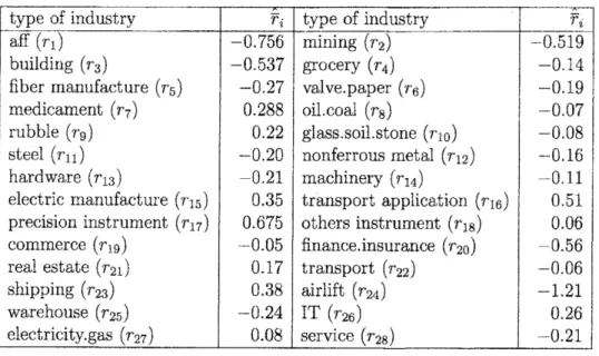
the monthly stock return data of various types of industries from January 1995 to December 2003. Weregard these 28 typesof industry indexes

as

28 kinds of risky securities. At first, we compute the 9-year average return rates by using 9-year monthly rate of returns to obtain $\hat{\overline{r}}_{i}$, $\mathrm{i}=1$, $\cdots$ ,28 (see Table 1). For

$\mathrm{e}\mathrm{x}\mathrm{a}$mple, the estimated mean rate of return on building industry is

$\hat{\overline{r}}_{3}$, and the

weight on the building industryin the portfolio investment is $x_{3}$. The

$\zeta" \mathrm{a}\mathrm{f}\mathrm{f}$” in Table 1 means the industry of

agriculture, forestry, and fisheries.

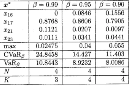
We use the SLP (Sequential Linear Programming) approach to derive an optimal portfolio of maximizing the CVaR-based Sharpe ratio. The computation are carried out based on

Al-gorithm 1 by utilizing the LP solver ofMATLAB 6.5 on a 2.60 GHz Pentiu$\mathrm{r}\mathrm{n}4$machine. The

optimal weights$x_{i)}^{*}\mathrm{i}=1$,$\cdots$ ,$n$, and the optimal number$K$ ofriskysecurities included in the

optimal investment

are

found out, and they are shown in Table 2. Then, for three different $\beta$-values 0.99, 0.95, 0.90,

we

also compute the $\beta-\mathrm{V}\mathrm{a}\mathrm{R}$ and $/3$-CVaR of the optimal portfolio $x^{*}$ as shown in Table 2. Further, in Table 2, _$N$ is the number of iterations required for the

convergence to the optimal solution. We find that the algorithm converges after 4 iterations for all $\beta$ values.

Table 1: Estimated Expected Rateof Return on Each Industry’s from Jan. 1995 to Dec. 2003 (%)

References

[1] Andersson, _{F. and Uryasev, S. (1999), Credit Risk Optimization with Conditional} Value-at-Risk Criterion, Research Report 99-9 ISE Department, University of Florida

Table 2: Maximal Value of CVaR-based Sharpe ratio, $x^{*}$, $\mathrm{V}\mathrm{a}\mathrm{R}_{\beta}$, and $\mathrm{C}\mathrm{V}\mathrm{a}\mathrm{R}_{\beta}$ Calculated by

Sequential Linear Programming Algorithm for $\beta=0.99$ 0.950.90 and $r_{f}=$ 0.0005, where

relevant

nonzero

$x_{i}\mathrm{s}$ are shown.

$x^{*}$ $\beta=0.99$ $\beta=0.95$ $\beta=0.90$

$x_{16}$ $x_{17}$ $x_{21}$ $x_{23}$ 0 0.8768 0.1121 0.0111 00846 0.S606 0.0207 0.0341 0.1556 0.7905 0.0097 0.0441 $\max$ 0.02475 0.04 0.055 $\mathrm{C}\mathrm{V}\mathrm{a}\mathrm{R}\beta$ $24.845\mathrm{S}$ 14.427 11.403 $\mathrm{V}\mathrm{a}\mathrm{R}\beta$ 10.8443 8.9232 8.0086 $N$ 4 4 4 $K$ 3 4 4

[2] Andersson, F., Maussef, H., Rosen, D., and Uryasev, S. (1999), Credit Risk Optimization

with

Conditional

Value-at-Risk, MathematicalProgramming, Series B, December

2000.

[3] Artzner, P., Delbaen F., Eber, J. M., and Heath, D. (1997), Thinking Coherently, Risk,

10, November 68-71.

[4] Artzner, P., Delbaen F., Eber, J. M., and Heath, D. (1999), Coherent Measures of

Risk}

Mathematical Finance, 9 203-228.

[5] Dinkelbach, Werner (1967), On Nonlinear Fractional Programming, Management Science,

13,

492-498.

[6] Stancu-Minasian, I. M. (1997), $Fract\iota onal$ Programming: Theory, Methods and

Applica-tions, Kluwer Academic Publishers.

[7] Sharpe, William F. (1994), The Sharpe Ratio, Journal

_{of Portfolio}

Management, Fall,

49-58.

[8] Markowitz, H. M. (1952), Portfolio Selection, Journal

_of

$F\iota nance$, 7 (1)

77-91.

[9] Palmquist, J., Uryasev, S., and Krokhmal, P. (1999), Portfolio Optimization with Condi-tionat Value-at-Risk Objective and Constraints, Journal

_of

Risk, 4, 11-27.

[10] Pflug, G. (2000), Some Remarks on theValue-at-Riskand theConditionalValue-at Risk,

in Probabilistic Constrained Optimization: Methodology and Applications (Ed. Uryasev,

S.), Kluwer Academic Publishers.

[11] Rockafellar, R. T. and Uryasev, S. (2000), Optimization of Conditional Value-at-Risk,

Jo\prime nmal

_of

Risk, 2, 21-41.

[12] Rockafellar, R. T. and Uryasev, S. (2001),

Conditional

Value-at-Risk for General Loss

Distributions, Research Report 2001-5, ISE Department, University of Florida, April, 2001.

[13] Uryasev, S. (2000), Conditional Value-at-Risk: Optimization Algorithms and