東北大学機関リポジトリTOUR

No 17 keV neutrino: Admixture < 0.073% (95%

C.L.)

著者

Ohshima T., Sakamoto H., Sato T., Shirai

J., Tsukamoto T., Sugaya Y., Takahashi K.,

Suzuki T., Rosenfeld C., Wilson S., Ueno

K., Yonezawa Y., Kawakami H., Kato S.,

Shibata S., Ukai K.

journal or

publication title

Physical Review. D

volume

47

number

11

page range

4840-4856

year

1993

URL

http://hdl.handle.net/10097/53659

doi: 10.1103/PhysRevD.47.4840

PHYSICAL REVIE%'D VOLUME 47, NUMBER 11 1JUNE 1993

ARTICLES

No

17 kev

neutrino:

Admixture

(

0.

073Fo

(95'Fo

C.L.

₎

T.

Ohshima, H. Sakamoto,

T.

Sato,

3.

Shirai, and

T.

Tsukamoto KEK, National Laboratory for High Energy Physics, Tsukuba 805, Japan

Y.

Sugaya and

K.

Takahashi

Tokyo University ofAgriculture and Technology, Tokyo 18$, Japan

T.

Suzuki

RIKEN, Institute ofPhysical and Chemical Research, Wako MI 01, -Japan

C.

Rosenfeld and

S.

Wilson

University ofSouth Carolina, Columbia, South Carolina 29808

K.

Ueno

University ofRochester, Rochester, Neur York 1$M7

Y.

Yonezawa*

Institute ofApplied Physics, University _ofTsukuba, Tsukuba 805, Japan H. Kawakami,

S.

Kato, S.

Shibata, and

K.

Ukai

Institute for Nuclear Study, The University of Tokyo, Tokyo 188, Japan (Received 12 January 1993)

Tosolve the controversial issue concerning the possible existence ofa 17keV neutrino with aleap

admixture innuclear _Pdecay, we_{searched directly for any evidence} ofaproduction-threshold effect. The Ni _Pspectrum was measured with a magnetic spectrometer, with very high statistics along with afine energy scan over a narrow energy region around the expected threshold. The obtained mixing strength was ~ U ~

=

[

—

0.

011+

0.

033(stat)+0.

030(syst)]'Fo, very consistent with zero, and

decisively excluding the existence of a 17keV neutrino admixing at the 1'Folevel with the electron neutrino. The corresponding upper limit was set at ~ U ~

(0.

073Fo (95% C.L.

).

A new limit was

also obtained for awider mass range: ~ U ~

(0.15'

(95FoC.L.) for 10.5to 25.0keV neutrinos.

PACS number(s): 23.40.Bw, 14.60.Gh, 27.50.

+e

I.

INTRODUCTION

Extensive experimental eKorts continue in order

to

probe the basic properties

of

the mysterious neutrinos. The current issues are related

to

their masses and flavor mixing. In addition

to

the solar neutrino problem, in particular, an experimental indication of a

17

keV neu-trino, reported by Simpson [1]in

1985,

has added fuel

to

neutrino studies. Various theoretical models _[2] have been proposed

to

accommodate such particles, while ex-perimental i.nvestigations have become controversial.

The current experimental situation regarding the

17

keV neutrino is illustrated in

Fig.

1.

There is a

'Present address: Tsukuba College ofTechnology, Tsukuba 305,Japan.

clear discrepancy between the negative [3—12] and pos-itive

[13

—17]results, which cannot be due

to

statistical fluctuations. One might say

that

since positive evidence has been obtained only in experiments using solid-state detectors, not using magnetic spectrometers, unknown detector-related phenomena are yielding an eEect which resembles

a

heavy-neutrino contribution.

If

so, the un-known phenomena have something

to

do with the specific energy

(17

keV) below the end-point energy since the pos-sible mass values so far reported are all around

17

keV [18],irrespective

of

the kind

of

nuclei used forexperiment. On the other hand, measurements using amagnetic spec-trometer have been criticized as having some ambiguities regarding the P-ray spectral correction.

The search for a heavy neutrino involves looking for some distortion due

to

neutrino mixing inthe P-ray spec-trum or an internal bremsstrahlung p-ray spectrum asso-ciated with some electron-capture process of radioactive nuclear decays. The flavor eigenstate could be

a

linear 0556-2821/93/47(11)/4840(17)/$06. 00 47 4840

1993

The American Physical Society

47 NO 17 keV NEUTRINO: ADMIXTURE &

0.

073go (95goC.

I.

.

) I I I I I

III„

(99~)

[3].

35S. M

[4],

35S, M

[5],

35S, M

[6],

35s,

s

[7],

35s,

s

6]

63Ni, M

[9]

125[ S

[10],

63Ni, M

[ii],

55Fe, S

[12],

35S, M

[13],

3H. S

[14],

35S, S

[i5],

35s,

s

[16],

~'Ce,

S

[17],

'4c, s

:

_(95')

THIS

EXPERrMENT, SSNi, M

I I I I I I II

0.

1% 1%

Mixing

strength

IUI

5%

combination

of

the mass eigenstates: I v,)

=

cos8

~ vi)

+

sin 8 I v2) if only two states are considered, where 8

represents the mixing angle. The

_P

spectrum would thus be

N(E)

=

cos

8Ni(E)

+

siil

8'(E),

N,

(E)

=

F(Z,

E)pE

(Eo

—E)

(Eo

—

E)2

—

m2

FIG.

1.

Experimental results concerning the mixing strength (I U I ) for 17keV neutrino. The arrows represent

the upper limits at the 90% confidence level (unless other-wise indicated), while the closed circles are from experiments reporting positive evidence. Indicated on the right are the reference, the P-ray emitter, and the experimental method. M and

8

represent amagnetic spectrometer and asolid-state detector, respectively. Our result is alsoindicated by the thick arrow.

understanding, the spectrum is usually presented in the form

of

a

Kurie plot:

gN(E)/[I'(Z,

E)pET]

vs

E.

It

forms a straight line if I U I

=0;

for I U I

$0,

however,

the slope for

E

((

E&h is difFerent from

that

for

E

&

Eth.

Although the experimental principle is very simple, get-ting

a

reliable measurement is not, as described below.

History is our teacher: forinstance, it had already been found 58years ago in 1934 [19),

a

few years after the birth

of

Fermi's P-decay theory,

that

Kurie plots

of

the mea-sured P-ray spectra were not as straight as theoretically expected. A noticeable excess was seen in the low-energy part of the spectrum. This discrepancy was

at that

time interpreted as being an indication

of

the necessity

to

re-vise Fermi's theory, not as asign

of

heavy-neutrino pro-duction. For example, Konopinski and Uhlenbeck [20] even proposed arevised theory in 1935in order

to

explain the experiment. Various investigations [21],which were carried out for over 20 years, finally revealed

that

the low-energy excess was the result

of

energy losses in the source substance and backscattering

at

the source back-ing plate.

It

is interesting

to

realize

that

we are again facing controversy concerning the P-ray spectral shape. This time, however,

it

isfrequently interpreted as arising from a

1%

admixture of

a 17

keV neutrino, thus causing some excitement among particle physicists.

We performed a measurement in order

to

clearly solve this controversial situation concerning the proposed 17 keV neutrino with

a 1%

admixture.

It

was aimed

at

achieving a sensitivity

of 0.1%

on I U I by directly

searching for a kink of the expected emission threshold in the ssNi

_P

_{spectrum with high} statistics and under well-controlled systematic conditions. Our experimental strategy

to

overcome the problematic aspects

of

previous experiments is described in

Sec.

II.

Descriptions of the experimental apparatus and the quality examination

of

the observed

data

are given in Secs.

III

and IV, respec-tively. Section V presents deductions concerning the

P

spectra and the response function. An analysis

of

the

P

spectra in terms

of

a y2 fit is performed in

Sec.

VI, but using a somewhat diferent method than

that

used in a previous publication [22]. Two analyses resulted in very good agreement concerning every fitting variable in detail. A further examination

of

the observed

_P

spectra is presented in

Sec. VII.

The search for a diferent mass of the heavy neutrino is also described in

Sec. VI.

II.

CONSIDERATION

(E

(

Ep

—

m,;

i

=

1, 2),

where p,

E,

and

ET

are the momentum, kinetic energy, and total energy of

a P

ray. Ep is the end-point energy

and

_{I'(Z, E)}

is the Fermi function. For the case in

ques-tion, the mass mi

of

the dominant neutrino, I

vi)

I v,

),

is set

to

zero and mass m2

to 17

keV. Thus, the minor

I v2) component should manifest itself as an excess over

the major term

at

an energy below its emission thresh-old, Eth

=

Eo

—

m2. Such an excess corresponding

to

sin 8

1%

was reported as positive evidence for a

17

keV neutrino [1,13—

17].

(In the following, the admix-ture sin 8is denoted by ~ U ~ .) For the sake

of

intuitive

A. Objectives

Loiii energy tail

of R(E')-and

the shape correction The true

_P

spectrum isdeformed due

to

the finite reso-lution

of

the experiment. This

e8ect

isrepresented by the response function

R(E,

_E),

which gives the probability for monoenergetic electrons

of

energy

E'

to

be detected at energy

E.

[For simplicity,

R(E', E)

is hereafter de-noted as

R(E)

throughout most part

of

this paper.] A

long, low-energy tail appears in

B(E)

due

to

energy losses and backscattering, which exhibits an approximately flat

4842

T.

OHSHIMA etal. 47

tail effect

6N(E')dE'

where

AE

=

(Eo

—

E).

In an experiment with a

_P

source separated from a detector, the backscattering gen-erates

a

tail with

a

size

of

20—30'%%uo of

R(E).

b' is thus

on the order

of

10 s (keV) . For example, 6' _(20—

30%)/(

150keV) for an s S source

(ED=167

keV). Then, the above-mentioned cumulative effect easily results in an excess

of

a few %, since the net effect is amplified by a factor of

LE,

which istypically afew tens of keV.

Such an excess atlower energies never disappears, even though it can be reduced by experimental efforts. Sys-tematic uncertainties usually limit any knowledge con-cerning 6

to

~

10

(keV),

thus leaving some

10

ambiguity in the measured spectrum, which cannot be ignored in

a

search for a heavy-neutrino effect

at

the I'%%uo

level. A so-called shape correction term is thus intro-duced

to

absorb this ambiguity. The term should never be omitted, unless experimentally justified.

8.

Statistical

balance and toide energy spectrum

energy distribution with an amplitude of6(keV) idown

to

zero energy. We also describe the fact

that

a

fraction of the

_P

rays

of

energy

(E')

flows into a data point at a lower energy

E.

By

approximating the true spectrum

N(E)

to

be proportional

to

the square

of

the energy in-terval from the end point,

Eo,

the fractional size

of

the tail contribution

to

the observed spectrum can be esti-mated as

Ep

near Eih in such experiments [13—

17].

A magnetic spec-trometer can considerably improve this situation.

B.

Experimental

strategy

Along with these considerations, we adopted a strategy

to

search directly for a kink due

to

the proposed

17

keV neutrino emission by means

of

a fine scan over the nar-row energy region in question with equally high statistics both above and below E&h. Any systematic uncertain-ties possibly arising from the energy-dependent charac-ter of corrections would not be

a

significant factor in

a

kink search. A kink, if

it

exists, would not be confused with the shape correction term. A very high-statistics measurement was made possible due

to

the combination of an intense source (ssNi) and a high-resolution mag-netic spectrometer. The signal-to-background ratio was as high as 1000near E~h, thus reducing the ambiguities in the background estimation

to

an insignificant level.

Another important feature of the present experiment is that

_R(E)

was precisely determined by a measurement, not by a Monte Carlo simulation. A monoenergetic _P emitter (ro9Cd) was used forthis purpose, which was pre-pared so as

to

yield the same energy-loss and backscat-tering effects as that of the 3Ni source.

The spectrum near Eo was also measured at

a

place where the shape correction is negligible and the

17

keV neutrino has no effect. The thus-obtained Eo value was compared, as a self-consistency

test,

with those deter-mined by

data

taken around E&h. The measurement was carried out using 30independent cells of a proportional chamber; this also helped in examining any systematic effects.

Most ofthe previous experiments measured some spec-trum over awide energy region, and used a

_y

fit over all parts in order

to

look for any difFerence in the slopes above and well below E~h, the threshold energy for heavy-neutrino emission. Nobody, except for Hetherington et al. [10], obtained sufficiently high statistics in the higher side

to

determine the slope there. In such data, the lower is the P-ray energy, the higher is statistical accu-racy, though the ambiguity islarger due

to

the tail effect described above. The situation isreversed at higher ener-gies. Consequently, the analysis becomes strongly biased by the low-energy portion of the

data

where the uncer-tainty islarge.

The above problem is not easily solved in experiments using

a

solid-state detector. The usable source intensity is severely limited by a signal pileup effect. Further, no

P

rays in an energy band

of

interest can be singled out.

8.

Signal-to-background ratio

Accurate knowledge concerning background is, need-less

to

say, the key for any reliable result. The determi-nation

of

the slope above Eqh is particularly affected by

the background. Experiments using solid-state detectors suffer from asignal pileup effect and residual radioactiv-ity. In fact, the signal-to-background ratio was only 6—60

III.

APPARATUS

A. P spectrometer

The P-ray momentum was analyzed by adouble

focus-ing

~~2-type,

iron-free spectrometer

at

INS (Institute

for Nuclear Study). This spectrometer had been success-fully used inprevious experiments [23] with athin tritium source in order

to

set the limit on the mass

of

the elec-tron antineutrino. The mean radius of the P-ray orbit is 75 cm, the main coil current is stabilized

to

within

10

and three sets ofHelmholtz coils (east-west, north-south, and up-down) can cancel an external magnetic field and its Huctuation down

to 10

of

the

10

G field applied

to

the

P

rays. The momentum resolution is controlled by a discrimination

baRe

slit located at 60 from the source position (see

Fig.

2).

For this experiment, the slit was adjusted so as

to

give

Ap/p=0.

2% and

a

solid an-gle of 0/4vr=4.

7x10 s.

The vacuum

of

the spectrometer chamber was kept at

10

3_—10

_Pa

_{during the entire}

pe-riod.

B.

P

source

We employed sNi _(wr~q

—

—

100yr) and Cd (wr~q——463

calibra-47 NO 17 keV NEUTRINO: ADMIXTURE

(0.

073% (95% C.L.) 4843

concerning the line shape and the count

rate.

The result verified good reproducibility in the source preparation.

C.

P detector

Gate Valve

ay

CB

Detector

FIG, 2. Top view of a vacuum chamber of the INS

m._{v2-type, iron-free spectrometer.} The _{momentum resolution}

is controlled by adiscrimination baNe slit.

tion

_P

emitters, respectively. Ni provides a 12-times larger rate decaying into energies near E&hthan does 3

S.

Well-known conversion lines

of

Cd decay provide us with a means

to

calibrate the system as well as

to

de-termine

R(E)

The two

.

sources were alternated several times during the experiment. The reproducibility

of

the source position was verified using the measured relative shift

of

the

K

conversion lines between different calibra-tion runs,

to

be better than &

+60

p,m, equivalent

to

LE

&

+2

eV at

E=50

keV. The sources were electri-cally grounded in order

to

avoid any charging.

Both

sources, each

of

4x20

mm2 size, were prepared on

a

1.

5 p,m thick Ni backing foil by an electroplating

method under the same conditions. An electrolytic so-lution

(0.

5 ml)

of 1%

ammonium lactate was used for the electroplating process with a constant 10 V applied for 15min

at

room temperature. The electric current in this process ranged from 40

to

80mA. The thus-obtained saNi _{source was 50} pg/cm2 in thickness and 580 pCi in intensity.

The Cd source of 150 pCi was prepared as

a

mix-ture with natural Ni atoms so

that

the energy-loss and backscattering efFects would be the same as those pro-duced with the ssNi _{source. The uniformity}

_of

_the mix-ture was confirmed in two ways.

₍₁₎

The electroplated efficiency was measured as a function

of

time by count-ing the

_P

intensity.

The

same efficiency was observed for two solutions (ssNi mixed with natural Cd and Cd mixed with natural Ni). (2) Another source was made by electroplating the correct amount

of

i09Cd and then natural Ni. The amount

of

the latter was

just

one-half

that

contained in the standard ~osCd _{source. Since} nat-ural Ni dominates the material in the standard o Cd source, this choice was made in order

to

mimic the av-erage energy losses encountered in the standard one. En

fact, the same

K

line shape was observed for the stan-dard and this test source. Finally, six Cdsources were prepared, and measurements were made for each

of

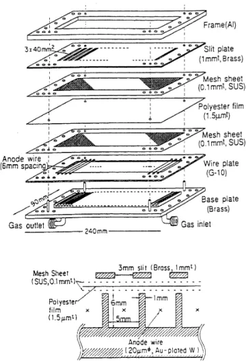
them

rame(AI) lit plate mmt, Brass) Mesh sheet 1mmt, SUS) olyester film 1.5pmt) Anode (6mm s 0 Mesh sheet .1mmt, SUS) 0/ire plate (G-10) l Gas outlet

~

240mm ase plate (Brass) Mesh Sheet (SUS,O.im ~) 3mm slit (gross PolyesTer film (I,5PrT)L)

—

+&

8—

1mrn y~&emm x Y

yx

Anode wire

p/ggggg/gg/ggy (Zap,m&,Au-platelet W

FIG. 3.

Structure and construction of the proportional chamber used as the P-ray detector.

The

_P

detector was a proportional wire chamber with 30 isolated cells placed on the spectrometer focal plane. Fig

3.

shows its structure. Signal wires were of 20pm rrrr

Au-plated tungsten, strung at 6 mm intervals. Rectan-gular counting cells

of

Gx6 mm each were formed by inserting 1 mm thick brass walls. Facing the incident

p

rays, an entrance slit

of

3x40

mrna opening was cut out for each cell on

a

1 mm thick brass plate. The slit size corresponds

to

the momentum bite

of

Ap/@=0.1'%%uo

or an energy bite

of

DE=96

eV

at

E=50

keV. Behind the slit plate was

a

1.

5 pm polyester 61m sandwiched by 100pm thick stainless-steel meshes of 95'Fo _in trans-parency.

It

isolated the chamber gas from the spectrome-ter vacuum and the inner mesh served as

a

cathode plane. The counting gaswas isobutane kept

at

4x

104

Pa

(within

l%%u~). A high voltage

of

1.

54 kV was applied in order

to

T.

OHSHIMA etal. 47 were mounted on the chamber. The position and angle

of the source and detector were optimized for the best momentum resolution by observing the ~ _Cd

_K

line. In this paper, the cells are numbered 1—30from the low-

to

high-momentum side.

D.

Data

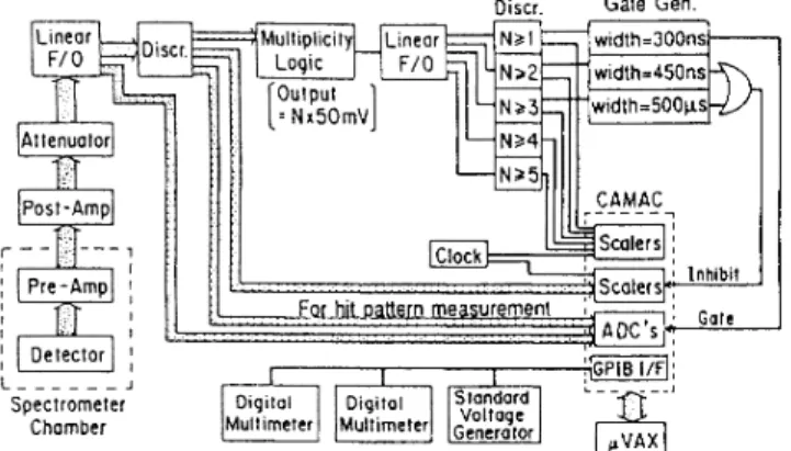
acquisition system

The electronics system is illustrated in

Fig. 4.

The overall gain in each pre- and post-amplifier chain was 12 mV/pA. Amplified signals were sent

to

analogue-to-digital converters (ADC's) (LeCroy

FERA)

for pulse-height measurements as well as

to

discriminators. The discriminator outputs were useful in three ways:

to

record the numbers of hits/cell by scalers,

to

register any event hit pattern by the ADC's, and

to

tag the hit multiplicity by the multiplicity logic module (LeCroy

380A).

Multiple hits were caused by cosmic rays,

elec-tronic noise, and cross talk; their rate was used

to

cor-rect for the dead time. Since electronic noise manifested itself as simultaneous trailing pulses on many cells, a 500 ps wide inhibit signal was generated on the multi-plicity

N &3. Its

contribution

to

the dead time, however, was negligibly small.

The magnetic field strength of the spectrometer was set by a standard voltage generator

(FLUKE

5440A). Using two digital multimeters

(FLUKE

8505A's), a yVax com-puter was used

to

monitor the generator voltage as well as the voltage across

a

standard resistor inserted in se-ries with the main coil, and thus controlled the generator accordingly.

illustrated in

Fig.

5, three sets

of

scans covered the energy regions of interest. Each set consisted ofmeasurements performed

at

20 magnetic fields approximately in 284eV steps for the Eqh region and the 4 magnetic fields ap-proximately in

7.

4 keV steps for the Eo region. In the former, the number of

data

points totaled (3 sets)

x

(20 magnetic fields per set)

x (30

detector cells)

=1800.

Of the 20points in each scan set, as can be seen in the figure, 3 points always overlapped with one or two other sets for normalization purpose.

At each magnetic field setting (thereafter expressed by the voltage across the standard resistor, V ~s), a mea-surement lasted 5 min, generating 30

data

points corre-sponding

to

the number

of

detector cells. In order

to

minimize any systematic errors, the V ~z value at

ev-ery scan was selected randomly. This was repeated until more than

10

counts had been accumulated at every data point, resulting in 2.

4x10

total

events over the

Eqh region where the signal-to-background ratio was as high as

1000.

Typical counting rates were 40 Hz and

0.

03Hz/cell at Ech and above

Eo,

respectively.

The Cd spectrum measurement was performed over a wide energy region from

16

to

107 keV in order

to

cover the

KI

I

Auger,

K,

I,

M

and N conversion lines. Different scanning steps were chosen, depending on the purpose: an absolute energy calibration, ameasurement of the spectrometer dispersion (dp/d2:, where

z

isposition displacement onthe detector plane), orameasurement

of

the response function. Figure 6shows an example ofsuch data recorded on the 16th cell. The counting rate was

IV.

DATA-TAKING

AND

QUALITY

EXAMINATION

20 points 20 points

20 points

A. Data-taking

procedure

The 6 Ni spectrum was measured in two different energy regions: One was around the expected heavy-neutrino emission threshold (called the Ech region) and the other was around the end point (the Eo region). As

Linear ~ F/0 ~oiscr

—

_ll

Attenuator ,' Multiplicity Linear Logic F/0 Output =_Nx5OmV

—

N&4-Discr. Gate Gen.

, N&1& 'width=300ns

=L

_{N~2 width=450ns} —Np3 width=500ps 284eV

steps

40 45

50

55

60

Energy

(keV)

Post-Amp 1 ( ; lpre-~mpl Detector, , ' L Spectrometer Chamber CAMAC ~scalersj', I Inhibit -- -=-',*',_Scolersi-, I Gate I' GPI8I/Fl, ' '

a'

I&lock,'

Fgrhitoattern measurement

I Digital Digital Standord ,Muttimeter Multime ter

Generator Voltage

R.VAX

FIG.

4. Electronics diagram.

FIG.

5. Illustration ofan energy scan performed around the 17keV neutrino threshold, Ebb=50 kev. Each of the three sets ofscans covered adiamond-shaped area, compris-ing (20

V,

s settings)

x(30

detector cells)=600 data points. The overlapped zones comprised three data points per detec-tor cell from each neighbor. The energy regions covered by the 16th cell are 45.9—51.3keV in

_(1),

41.4—46.5 keV in _(2), and 50.7—56.3in

_(3).

The four points in the Ep region, not illustrated, covered 65.4—87.6keV in

_(1),

68.9—

91.

5 keVin _(2), and 63.7—85.7keV in

(3).

47 NO 17 keV NEUTRINO: ADMIXTURE &

0.

073%(95goC.L.) 4845 1

(141)

2

₍₁₄₂₎

3

(142)

4 (142) O

0

2000—

10QO— KLL Auger I KLM8cKLN Auger ) K line Lline M line &~N line

30—

zo—

10—

0 I

3

I 5 (142) 6

(142)

7

(142)

6 (142)

30—

zo—

10—

80 40 60 80 100 _o

Energy (keV)

FIG.

6. Cd spectrum measured inthe 16th detector cell, showing discrete lines and their tails used for calibration pur-poses.

2.

2kHz/cell

at

the peak

of

the

K

line. The measurement was performed four times during

a

2-month data-taking period, each lasting for 2

to

3 days.

The background was studied without the source, or by closing gate valves

at

either the source chamber or the detector chamber. Since

it

was mostly cosmic rays, the rate did not appreciably depend on how the

P

rays were shut out. In addition, this rate fairly well agreed with those observed above Eo

()67

keV) aswell as above the Cd

N

line

()88

keV) where no

_P

rays should exist.

9 (142) 10 (142) 11

(142)

12 (142) g

30—

20—

10—

0 I I —5 0 I I I 5 —5 0 I I 5—5 I 5 —5 0 Devia.

tion

FIG. 7. Distributions of the counting rates (n's) rela-tive to the average (n). The horizontal axis corresponds to (n-n)/Vn. The data are from the 16th detector cell, in data set (1)at 12difFerent _{V s settings. The}curves are Gaussians ofunit standard deviation, with areas equal tothe number of runs shown in parentheses.

B.

Data

equality

X. '81Vi data

As explained above, each

data

point is

a

result

of

many runs performed in random order. The run-to-run stability

of

the counting rates in individual

detec-tor

cells should be

a

good measure

of

the

data

quality. The histograms in

Fig.

7 show distributions

of

the rates

(n's) recorded under identical conditions. The curves are Gaussian distributions normalized

to

the respective num-ber

of

runs. One clearly finds only statistical fluctuations without any

extra

disturbance. This is also true for all

of

the other data not shown in the figure. The count-ing rates

of

all runs

at

600 individual

data

points, (20 V~ g's)

x

(30 cells), in the Eth region were further exam-ined in terms

of

the reduced yz:

(reduced

y

)—

:

)

.

(n

—(n)&'

run &

)

[(the number of runs)

—

1j.

Here, (n) corresponds

to

the average of the rates

at

each

data

point, and isdetermined by minimizing the reduced

y

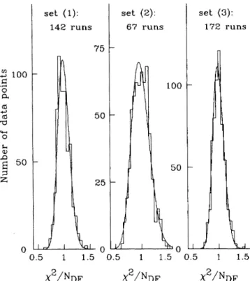
. Figure 8 shows the reduced

_y

distributions for the three sets

of

scans. The curves represent ideal

_y

dis-tributions and show

that

the

data

scatter in a purely statistical manner.

As shown in

Fig.

5, three sets

(1,

2and 3) of scans were carried out in random order for individual points, with an overlap in two bands. The ratio

of

the summed counts in these bands should depend only on the data-collection time and the ssNi lifetime. The experimental values are

I

0.42430+0.

00006

for

_(2)/(1)

and

1.32809+0.00018

for

(3)/(1),

which are in very good agreement with the ex-pected

0.

42445

and

1.

3299.

Because there was ascheduled electric power outage after scans (1)—(2), the comparison ofthe absolute rates between (1) and ₍₃₎gets a bit poor. But, it does not influence this experiment. The Cd calibration runs were therefore per-formed before and after the both (1)—(2) and (3)scans

4846

T.

OHSHIMA etaI. 47

set

(1):

142 runs

set

(2):

67

runs

set

(3):

172

runs

100

0

Q

0

50

25—

100—

50

o I

0.

5 1

1.

5

0.

5

1.

5 0

0.

5 1

1.

5 X /NDF X /NDF

x

/NDF

FIG.

8. Histograms ofreduced _y defined by Eq. (3)for three data sets, each with 600data points. The curves repre-sent ideal distributions for Gaussian distributed variables for the corresponding number ofruns.

It

is thus concluded

that

the entire experimental sys-tem has been stable and

that

the final spectrum can be obtained by summing all

of

the counts in each

de-tector

cell

at

the same V _~+ without making any

time-dependent corrections. A single scan set lasted for about 2 h

at

over 24 different V~~z settings with 5 min each. The long life

of

Ni does not require any correction for this time period, and the random sequence in the indi-vidual settings further reduced the effect of the source lifetime.

It

can also be concluded

that

the source did not evaporate in avacuum, contrary

to

other cases [8,

12].

V.

DATA

REDUCTION

We aimed

at

precisely measuring the shape

of

the 3Ni P-ray spectrum, not the absolute decay

rate.

Therefore,

Of the four calibration data sets with the resCdsource, both the first two and second two were taken

at

29—30 day intervals. The source lifetime is not negligible here when comparing the

data

sets. The observed ratio of counts at around the

K

line is

0.

9568 between the first two and

0.

9569 between the second two, while

0.

9561—

0.

9575is expected for both from the decay in the source intensity. This agreement again confirms the stability

of

the system, as already shown using the Ni

data.

It

also shows

that

no appreciable source evaporation occurred.

energy-dependent corrections were important, such as the electronics dead time, transmission through the

de-tector

window, and any loss due

to

pulse-height discrim-ination. The Cd spectrum was used for absolute-energy calibration as well as

to

establish the spectrometer dis-persion. The response function

_[R(E)]

was also obtained

from the same

data.

Finally, the Ni P-ray spectra in 30

individual cells were arranged for subsequent analyses.

A. Corrections

1.

Dead time correction

The sealer counts of 30 cells at every V _~ setting were normalized by the live-time interval. Only single-hit events were counted in order

to

reject electronic noise, cosmic rays, and cross talk. The number ofinhibit sig-nals generated on multihit events was also recorded in order

to

evaluate the electronic dead time. The result-ing dead time correction was on the order of

10

for 20 points in individual

data

sets, each covering approxi-mately a

5.

4keV interval near Eqh.

Its

variation between the lowest- and highest-energy point was

3x10

4 _{for set}

(1), 4x10

4 for

(2),

and

2xl0

4 _for

_(3).

_{Consequently,}

this correction of the 3Ni _spectral shape amounted

to

only &

+2x10

over the

5.

4keV interval near E&h. The correction near Eo was even smaller, being on the order

of

10-'.

2.

Count Lo88 due to discrimination

e(E)

&max

h(E,

c)dc

&max

h(E,

c)dc, (4) where

h(E,

c) represents the count in the cth ADC bin for the P-ray energy

(E)

and h isthe average

of

20

spec-tra.

e(E)

depended slightly on the range of integration. The choice

of

c

=9

was made in order

to

make it sensi-tive

to

any discrimination efFect. The result isplotted in

The background pulse-height distribution inthe cham-ber was determined from

data

taken

at

two V _~gsettings, where no P rays from the source were expected. Figure

9(a)

shows a typical background-subtracted pulse-height distribution for the Ni source. One can see a discrimina-tion level corresponding

to

ADC channels of 10or below; the loss due

to

discrimination is therefore only a small fraction of the

total

events. What is relevant in this ex-periment is the P-ray energy dependence of this small fraction.

The low pulse-height part is shown in

Fig.9(b),

where 20spectra corresponding

to

20 consecutive V _~ settings in one of three data sets are plotted forthe same detector cell, and the histogram is their average. The fraction of counts in this part does not show any noticeable depen-dence on the P-ray energy (or V ~s). To determine the possible energy dependence ofsome discrimination effect, the count integrated over low ADC bins was studied rel-ative

to

the average, by defining

47 NO I7keV NEUTRINO: ADMIXTURE &0.073% (95% C.

L.

) 4847

15000

10000

5000

0 0

0.

015

0

0.

010

a

0.005

0

0.000

(b)

100

ADC

channel

I 10 20 ADC

channel

200

Semiempirical equations exist

that

relate the electron energy and the extrapolated range [24], and

that

repre-sent the transmission [25]. Equations

(6)

and

₍₇₎

in Ref. [24] well reproduce many experimental data; however, as the authors pointed out, they are not in perfect agree-ment with each other. This uncertainty corresponds

to

approximately

+4%

in our film thickness, while the ac-tual thickness is uncertain

to

+3%.

Thus, by quadrati-cally adding these uncertainties,

+5%

was assigned as a systematic error in the film thickness.

Figure 10 shows the thus-calculated transmission through the

1.

5 pm film, which is

98.1% at

E=40

keV

to 99.3%

at

E=60

keV. The range

of

uncertainty is also

shown there, and is smaller than

+1

x10

in the Eih-region. This correction was also applied

to

the Cd spec-trum.

B.

Energy

determination

1.

05 Qp —~.p T~ IP ~ ~~ ~~ II II sa. %F

0.95

I

46

I 48

50

Energy

(keV)

FIG.

9.

(a) Background-subtracted pulse-height distribu-tion for the 15th detector cell measured at the 10th V setting in data set

(1).

(b) A closeup ofthe low pulse-height region of

(a).

The dots are for 20different V~~s settings and the histogram shows their average. (c) e(R)defined byEq.(4) at individual V _~ values, thus at different

E.

The solid line is afit to the data.

X. Dispersion relation

=

_(U~

_i;„,

_)is

_(V)

[1

+

a(j

—

16)

+

5(

j

—

16)

+c(j

—

16)

].

(5)

The sizes of the coefBcients determined in the first cal-The momentum dispersion

of

the spectrometer was established by determining the Vm~g value) V~ ]I„p&

at

which the Cd

K

line peak appeared in

a

given detector cell. For this purpose, by changing Vm@g the position

of

the

K

line was moved across all

of

the cells. The accuracy in this measurement was

+(1

—2) eVin energy. The result was fit by

a

fourth-order polynomial

of

the cell number

(j),

where the 16th cell was taken as

a

reference:

(I

Kline)

j(~)

Fig. 9(c)

as

a

function

of

E.

The linear fit shown in the same figure gives the energy-dependent contribution

to

the low pulse-height part

to

be smaller than

+1%/keV.

The

total

loss

of

counts in this pulse-height region was

(1.5+0.

4)%,

by linearly extrapolating the counts

at

c

The uncertainty resulted from the fact that the choice

of

c

is not unique. The final correction factor is there-fore less than

(1.

5+0.

4)

x10

4/keV. The same correction was also applied

to

the Cd spectrum, although it is much smaller than the statistical errors.

8.

Z'ronsmission

_of

detector isindoiii film The only material

to

beconsidered is the

1.

5 pm thick polyester used as the detector window, since the meshes have

a

fixed transmission, irrespective

of

the p-ray en-ergy

of

interest. The chemical structure of the film is Cz+ip He+s~Og+4~ and the density is

1.

393

g/cm For sufBciently large values

of

n, the effective atomic and mass numbers are

Z,

a=6.

45 and A,

@=12.39,

respec-tively. The ambiguities in the n value has totally negli-gible effects on the transmission.

1.OO0 a.995 0.990 0.985 0.980 O.975 0.10 0.05 0.00 —_0.05 —O.

&0—

40 l 45 50

Energy

(keV) ! 55 60

FIG.

10. (a) Calculated P-ray transmission

[T(E)]

for a

1.

5 pm thick polyester film. The thin curves show the range ofuncertainty corresponding to

+5%

ofthe nominal thick-ness. _{(b) The} range ofrelative uncertainty when normalized at

E=50

keV.

4848

T.

OHSHIMA etal. 47 ibration run came out

to

be

a

=

—

1.

95023x10,

6

=

6.

34526x10,

and

c

=

3.07130x10

.

They agreed

very well with the analytic orbital calculation.

The same measurement was performed in every cali-bration run. A slight variation which depended on the run was detected in the V _gvalue forthe

K

peak at the reference cell, and was attributed

to

asource replacement error.

By

examining the relative shift

of

the

K

and

I

lines, the errors in position were found

to

be

+15

pm be-tween the first two calibrations and

+60

pm between the second two. They correspond

to

an energy uncertainty of

+0.

6eV and

+2.

4eV

at

K

line energy.

8.

Abaolute-energy calibrution

To relate _V~~s

to

the P-ray momentum, the

K

and

L

lines, aswell asthe

KLI

lines, were measured bythe 16th cell in every calibration. Their energies (and relative in-tensities) are known with accuracies

of

0.

3—

0.

4eVfor the

K

and

L

lines [26] aswell as

1.

3

—

1.

7eVforthe

KLL

lines [27]. In our measurement, the

K

line,

E~=62.

520 keV, was measured with an accuracy

of

+0.7x10

in V _~~, or

+0.

8 eV in energy. A fit was made

to

the

L

line

data

based on the observed

K

line spectrum, rescaled by taking into account the energy differences, the rela-tive intensities

of

the

I

sublines, and the different energy losses. The result was accurate

to

+3.1xl0

5 _{in V}

z,or

+4.

9 eV in energy, at

EI.

,

=84.

683 keV. The

KLL

Auger spectra were fit by

a

functional form used in Ref. [27]; the KLqL3 line,

E~g,

L,

,

=18.

512keV, was determined

to

be

+6.

8x10

in V _z or

+2.

5eV in energy. The result isexpressed as

served near 53and 72 keV, which could be backscattered

P

rays of the

K

and L lines, respectively. Because

of

this efFect, the tail shape, expressed as

_{exp[(Eb„~ —}

E)

s],

where

Eb„p

represents the position of the bump, was found

to

reproduce the

data.

Several different functions were also used

to

evaluate the uncertainty in the subtrac-tion. Figure

ll

is

a

result

of

such an evaluation, showing the possible variations in the tail spectrum. This un-certainty was treated as one

of

the systematic errors in the final analyses

to

be described later. The high-energy side

of

the resulting pure

K

line shape was also checked by comparing it with

that

of

the

N

line, which is at the highest energy receiving no contribution from other con-version lines.

Figure

11

shows the thus-obtained

K

line spectrum.

It

is equivalent

to

the response function

_{R(Ea, E)}

for

P

rays

of

energy

Ea.

The low-energy component re-fiects the backscattering and energy-loss efFects. This response function was applied

to

other P-ray energies by

just

rescaling it in momentum.

D.

S~Ni

_spectrum

After applying the conversions and corrections de-scribed above, the counts recorded under the same condi-tions were summed. As described before, there were 1800 data points near E&h, and 360data points

at

around

Eo.

The three sets

of data

were normalized using the counts in the overlapped region, three points from each

set.

The

p(keV/c)

=

187.

6650 x

V,

s(V)

+

0.

3070 (6)

x

]05

for the 16th cell. This relation was valid for all

of

the calibration runs within

+1

eV accuracy and, therefore,

at

all of the energies covered by Ni runs.

Equations (5) and (6) were used

to

convert the V _~s value ofeach

data

point

to

the energy

E.

The measured counts

at

all

of

the points were then corrected so as

to

have the same energy bin size.

C.

Response

function

Because of the optical characteristics of the spectrom-eter, there is a very small cell dependence in

K

line spectra. The momentum resolution [Ap/p full width at half maximum (FWHM)] varies parabolically from

0.

26% at the 16th cell

to

0.

29% at both ends

(1st

and 30th cells). In more detail, their half width at half maximum (HWHM) remains constant

at

the higher-momentum side, but has acell dependence

at

the lower side. There-fore, both Ni and Cd spectra measured in individual cells were separately treated in the following analyses.

To

extract

only the

K

line spectrum from the data

(shown in

Fig.

6, for example), the low-energy tails of the L and higher lines must be subtracted. They were assumed

to

have the same functional forms as

that of

the

K

line. Inthe spectrum, small but broad bumps were

ob-xQQ

I I

40

50

Energy

(keV)

FIG.

11.

Response function

[R(E~, E)]

extracted from the Cd P spectrum, shown by a curve with data points. The size of the ambiguity resulting from subtraction of the L and higher line components is indicated, by adding to the

47 NO 17 keV NEUTRINO: ADMIXTURE &0.073% (95% C.

L.

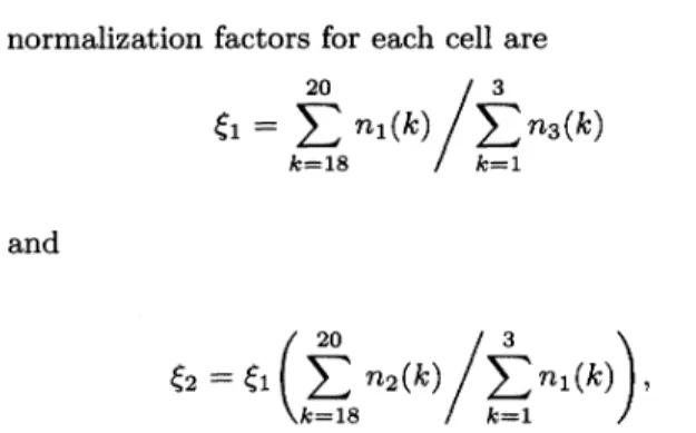
) 4849 normalization factors for each cell are

20

g,

=

)

n,

(k)

)

n.

(k) k=18

A.

Formula

The following formula was used

to

fit the

data:

N

'(E) =

Ap

[N'"(E')(1+

n(Ep

—

E'))R(E',

E)]dE'

(7)

_+B(E),

₍₈₎

2p

(g

—

—

qi

)

n2

(k)

)

ni

(k)

(A'=is k=1

where

n;(k)

are the counts

of

the kth data points in the ith data set

(i=1,

2,

3).

Furthermore, the spectrum ofeach detector cellwas normalized

to

the 16thcell by equalizing the summed counts in the same energy ranges. The final spectrum in the Eqh region is shown in

Fig. 12.

VI.

y~

ANALYSIS

N'"(E')

=

I'(Z,

E')p'ET

.

(

(1-

I U

I')(E.

—

E')'

+

I U

I'

(E,

—

E')

_(E.

—

EI)2

—~2

(9)

where ET is the total energy

of

the

P

ray, Ap is the

nor-malization constant, and cristhe shape correction factor.

I U I2 expresses the mixing strength

of

a heavy neutrino

ofmass rn H.

F(Z,

E)

is the radiatively corrected, rela-tivistic Fermi function [28]. The background spectrum is represented by

B(E),

comprising

a

constant and

a

small linear term.

The narrower the energy range analyzed is, the smaller the ambiguities in energy-dependent corrections are. The spectra in the Eqh region and the Ep region were therefore analyzed separately. The

E0

value extracted from the latter was used

to

assess the result from the former. The following analysis is different from

that

reported in Ref. [22] in treating the normalization constants,

(i

and

(z.

However, the result is not significantly different.

x&O6

B.

Eo region

The three sets

of

scans made

at

around the end point (Ep) were combined into a single spectrum by using the normalization factors

_(i

and

_Q

in

Eq. (7) that

were eval-uated from the data near

Eth.

Ambiguities arising from this procedure are negligible compared

to

the statistical accuracies

of

the data in question.

In the energy region near

E0,

the shape correction fac-tor (a.) has only a small effect.

The

low-energy tail of

R(E)

also plays aminor role in the integration

_{of Eq. (8),}

since the energy range

to

be considered here is narrow. In addition, the emission threshold (Et,h) of the heavy neutrino is much lower. Consequently, one can deter-mine

a

reliable value for

E0

under clean circumstances.

It

would provide us with

a

very valuable means

of

making consistency checks on our analyses

of

the entire spectra. A g2 fit was made

to

the spectrum between 63 and 74 keV with both

n

and I U I set

to

zero. The fitting

variables were Ap, Ep, and two parameters of

_B(E).

The result is shown in

Fig. 13

and the best-fit value is

Ep

=

(66 945.9

+

4.

4) eV,

with

_y

/NDF(number

of

degrees

of

freedom)

=116.

6/102.

A similar fit was repeated with and without cr as an ad-ditional parameter and by changing the low end

of

the fitted data points in

0.

5keV steps from

62.

0

to 64.

5keV. The resulting values

of

Ep and

B(E)

were very stable. Therefore, the background

_B(E)

determined here was used in the following analyses. The value

of

a

was con-sistent with zero with large errors.

p I

40

I I I

45

50

55

Energy

(keV) I

60

_C.

_Individual

_{Bts for}

X~h region

FIG.

12. Ni spectrum measured around the 17keV neu-trino threshold _(Etq), consisting of1800data points. See the text for details.

30 sets

of

spectra, each consisting

of

60

data

points

at

around Eth, were individually analyzed under the as-sumption

that

m~H

=17

keV. The normalization factors

4850

T.

OHSHIMA etal.

((i

and

₍₂₎

were not applied here. Instead, the following six parameters were treated as being free: I U

I,

o.,three

normalization constants [2~0

(j=l,

2,3)]corresponding

to

the three sean sets, and

Eo.

Other cases were also exam-ined with Eobeing fixed

to

the measured value [Eq.

(10)j

or with I U I set

to

1%.

Figure 14 compares the best fits and the

data:

(a)

for six parameters and _(b) for five parameters with

I U I

=1'%%uo. For case

_(b),

the fit clearly becomes worse

near 50 keV, the expected neutrino production thresh-old. The qualities

of

the fits are shown in

Fig. 15(a)

as the reduced y2 values for the 30 spectra. Systematically larger yz values are seen for the case with I U I =1'%%uo.

The best-fit I U I values are plotted in

Fig.

15(c).

The

average over the 30individual results gives

6 —

x10

(I U I )

=

(

—

0.

029+

0.

038)%

with

_y

/NDp=1.

13 (NDp=29).

It

isconsistent with zero; in fact, the average of the reduced

_y

values is

1.

01for

I U I being free, while it jumps up

to

1.

45for I U I =l%%uo.

The five-parameter fit with Eo fixed also leads

to

(I U I

)=(

—

0.022+0.033)%

with

g

/NDp=1.

26.

The other parameters determined inthe fitsare plotted in

Fig. 16.

When I U I is left free, the average of 30 Eo

66

68

70 72

74

Energy

(keV)

FIG.

13. Ni spectrum measured near the end point, Eo. The curve isthe best fit which gives aprecise value ofEo.

0.005 — 13

(1.

233) 16 (0.786) 13

(1.

939)

16

(1.

542) 0.000 f ilI il I I I,lIIII I QIll I III il I ~ il _y II I _JI IliIi III

II _..1IIIJ%iI _III II~IliIl ilIIIiiIIii Il 'lI il II)IIIIl illl' II il ll I~1III il II .i'll 'l..Ii ii'IIIli il ll _II

'_IIII"IIiII_)II

'

IIIII II I1I 1/111II ii11~ ~ —_0.005 0.005 — 14

(0.913)

i7

(i.

03i)

14

(1.

730) 17

(1.

540) I A 0.000 il II ll 1 I Ii il Il 11 II l11 JJIIII ll II illlil il i I I I illI II ll I il ii i iiI iI II ll III il..)' ~i&ll II II II II il II iII il , g,ii"o11 ~I III III1 II 111 iil' II il 111 I ilil ll li ]y~ ~I 111 il 11 il II iIII —0,005 0.005 — 15

(1.

077) 18

(1.

008) 15

(1.

780) 18

(1.

766) 0.000 il ii II Jpll (li il IIIill 'll ' Il I& I I I III't _Q iI 1I II II ill il il II II ll illl illIl ll II iI il il ii iII il II

II_IIi I

il"'

iiIII1,„il.. II

[ ~~ i1 II ~I Ill 1I IIllI IIII il '1l ll il Illi ii il Illl,i ill ilill.II !' il 'll _ll IIIIIIII 11 III ii illi iII II _II il —_0.005 40 I 50

Energy

(keV) I I 55 40 I 45 50 Ener _gy (keV) I 55 40 45 50

Energy

(keV)

I I 55 40 45 50 Ener gy

(keV)

I 55

FIG.

14.Examples of the fitstoindividual Ni spectra measured in the energy region around E&p. Six spectra corresponding tothe detector cells from the 13th to the 18th are plotted relative to the best fits. (a)and _(b) show the results of the fit with

I U I left free and with I U I =1'%%uo, respectively. Shown at the top ofeach spectrum are the cell number and the reduced y

NO 17 keV NEUTRINO: ADMIXTURE

(0.

073% (95% C.

L.

) 4851

(a)

_(b)

C& C& I CO 200 Ii IIli][ il

)

IIII

f

f —₁₀₀ —

_(a)

0 i 0.5 V (g

0.

0 II Igl /I II II IIII II Ii II I 2 4 6 Number of

cells

—20

(b)

IiII il Ii II II wr —

_0.

₅ —_1.0 I 0 j I iO 20 Cell number I 30 1.002 1.000 C0

0.999

~~~ ~~ ~~ II II ~fl ~~~II() I)~ IIII/ $() () () ~~~~~ ~iiI ~~II~ () () II .

.

()II c&

II.ll.(il

.

)g

. .

„.

~I.

'

Ii IiIl

FIG.

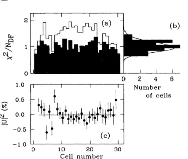
15. Result ofindividual fits. (a) Reduced ₎₍ values where the closed histogram comes from afit with i U i left

free and the open histogram from the fit with i U i =1%%uo.

The distribution ofthe )( values are plotted in (b), where the curve represents an ideal one for a Gaussian distributed random variable for No@=54. (c)The best-fit i U i values.

1.002 CO

0.

998 C3 ~~ _{II I 0}~~ ~ 1.000 ~()~ g)q) ~ ~ () II _II a~~ s~~ ~ ~~ II II ~I')I)~₍₎~~()I_if ~iiII

(c)

. .

.

.

.

,

.

ji.-~ ~~ 0~ ~~~ ~~i~ ~)I

(d)

values is (Ep)

=

(66 942.8

6

5.

5) eV, 10 20 Cell

number

30

D.

Global fits for

the

Eth region

Next, a global fit was performed

to

all

of

the 1800data points with 122 fitting parameters: n and A~&

(j=1,

2,3)

for each detector cell and two common variables, Eoand

i U i . The best fit shown in

Fig. 19(a)

resulted in

i U i

=

(

—

0.

011

+

0.033)%

(13)

which agrees very well with the measured

Ep=(66945.

9+4.

4) eV, [Eq.

(10)j,

as can be seen in

Fig.

16(a).

On the other hand, if i U i is set

to 1%,

the resulting average Eo is lower by

61.

5 eV. The size

of n

given in

Fig. 16(b)

is on the order of

10

4 _(keV)

when i U i is left free. Finally, two ratios of the

normal-ization constants, Ap/Ap

sand

Ap/Aps, are comPared with those independently evaluated in the previous section in terms

of (1

and

_(z.

Figures

16(c)

and

_16(d)

show such a comparison. The dotted lines indicate the statistical uncertainties involved in the (' values. The two difFer-ent methods

of

normalization give consistent results only when i U i is not fixed. In conclusion, the cases with i U i

=1%

are significantly disfavored in several aspects:

y,

Eo,

0,as well as the normalization.

Figure

17

displays the variation

of

yz with i U i

z_forthe

30 spectra, showing

that

the

_y

minima are well defined and

that

all of the best-fit values cluster around zero. Correlations between the variables are shown in

Fig.

18 as

_y

contour plots: n-i U

i,

n-Ep, and Ep-i U i

FIG.

16.Various parameters resulting from individual fits, made with i U i left free (closed circles) and with i U i

=1%

(open). (a) The end point energy. The line is the one deter-mined from the data taken near Ep itself, Eq.

(10).

(b) The shape correction factor

n.

(c)and (d) Ratios ofnormalization constants for three data sets, compared with those

_((i

and (2) obtained from the counts in the overlapped region. The dotted curves indicate the statistical uncertainties involved in

('s.

Ep

=

(66943.

3

6

4.1)

eV,

(14)

with

yz/NDF=1701.

1/1678=1.

01

(also see

Fig.

20).

All

of

the other parameters turned out

to

besimilar

to

those obtained from the individual fits. The curve simply il-lustrates the size

of

the hypothetical 1'%%uo mixing for the

17

keV neutrino. When i U i was fixed

to

1'%%uo, the

resulting Eo

—

—

66882.

3+4.

6 eV was oK by

63.

6 eV from

Eq.

(10),

and the fit was considerably worse, as can be seen in

Fig. 19(b),

giving

_y

/NDF

=2466.

9/1679=1.

47.

It

should be noted here

that,

as the figure shows, since the statistical weight

of

the

data

points was well equalized over the whole energy region, the fit was not locally bi-ased. The result

of

the global fit,

Eq.

(13),

agrees very well with

Eq.

(11)

obtained from the individual fits.

Possible sources

of

systematic errors are the remaining ambiguities in the P-ray transmission through the

detec-4852

T.

OHSHIMA etal. 47 All

of

the results described in this section aresummarized in Table

II.

E.

Search

for

a

difFerent mass

of

the

heavy neutrino

A global fit was also performed while searching for heavy neutrinos

of

different mass.

Fit

and error evalua-tions were carried out in the same manner as described above. Figure 21shows the best-fit ~ U ~ values as well

as the

95%

confidence upper limit on them. Where the fit resulted in

a

negative value

of

~ U

~,

it

was set

to

zero

in evaluating the corresponding limit. No evidence was found for heavy neutrinos, Inconclusion, the upper limit on the heavy-neutrino admixture is

0.

15%

(95% C.L.

)in the mass range

10.

5—25.0 keV.

—

_0.

₀₂ —

_0.

₀₁

l

0.

01

l

0.

02

VII.

DISCUSSION

A.

Normalization

FIG.

17. _y curves vs ] U ~ for individual spectra

(NDi;=55 each). The closed circles are the best-fit ~ U

values.

~ U

~'

=

_[

—

_0.

011+

0.033(stat)

+

0.

030(syst)]%

(15)

~ U i

(0.

073%

(95% C.

L.

).

(16)

tor window, the low-energy tail of the response function

[R(E)]

and the background shape

[B(E)].

To evaluate their effects on the final physics outputs, fits were made by varying the individual factors within the ranges esti-mated in

Sec.

V.

The results are listed in Table

I.

The overall systematic errors were obtained by quadratically adding these uncertainties, giving

+0.

03%

for

~ U ~ and

+11.

5 eV for

Eo.

Consequently, our final result for the

17

keV neutrino is

The energy region around Eth was measured by three partly overlapped sets

of

scans; therefore, two normal-ization factors were introduced in the fits described in the previous section. In

a

previous publication [22], on the other hand, the normalization had not been treated as free parameters. Instead, it had been uniquely deter-mined by calculating the

_(i

and (2 as given by

Eq.

(7).

These different methods were systematically compared in this paper, as already shown in

Fig. 16.

It

is concluded that the physics results do not depend on the normaliza-tion method.

B.

Smoothness

of

the spectrum

The heavy-neutrino component near the emission threshold should exhibit an energy dependence

that

is quite difFerent from the shape correction term. Infact, as already shown in

Fig. 19(b), a

fitwith ~ U ~

=1%

resulted

0,

01

0.

01

G?

—

0.00

—

0.

00

—

_0.

₀₁ —

_0.

₀₁

—

_0.001

_0.

₀₀₁

n

(1/keV)

—

_0.001

₀

_0.001

n

(1/keV)

EQ

(keV)

FIG.

18. _y contour curves for the spectrum measured by the 16th detector cell, showing correlations between the Gt

parameters; (a) ~ U ] vs

a,

(b) Eo vs

a,

and (c) ] U ~ vs Eo. The contours correspond to b,g

=y —

y;„of

1,1Q, 5Q, 1QQ,

NO 17 keV NEUTRINO: ADMIXTURE &0.073% (95% C.

i.

.

)

0.

008

I (Q

0.

004

0.

000

-0.

004

0.

004

0.

000

A —

_0.004

40

[ 45

Energy

(keV) [

50

I

55

]

60

FIG.

19.The data in the Eqh region plotted relative to the best global fit, (a) mith ] U ] free and (b) ] U ]

=1%.

For the

sake ofillustration, deviations of data points are binned into every 50 eV. The curve in (a) illustrates the size ofa 1%mixing effect of the 17keV neutrino.

Source ofambiguity Window film thickness Tail in

R(E)

Background shape

B(E)

TABLE

I.

Evaluation of systematic ambiguities. Change in parameter Effect on ~U

],

Ep

+5%

—

0.024%,

+5.

2eV

—

_5%

_+0.

_002%,

—

_{5.9 eV}

Positive side (Fig. 11)

+0.

018%,

—

8.3 eV Negative side (Fig. 11)

—

0.037%,

+11.

9 eV

Negligibly small for NDF

—

—

1678 1701.0 1701.8 1702.9 1701.5

TABLE

II.

Results ofvarious fits with m H

=17

keV. The number in angular brackets is the

average of the 30resultant values obtained by the individual fits. Details are described in the text.

x'

I U I' (%)

Fit near Eo

116.6 102 fixed to 0.0 45.

9+4.

4 Ep

=

[66945.

9+4.

4(stat)

+3.

2(sys)] eV Individual fits

near Eth Fixed to

1.

0

(-0.022+0.033) Fixed to

1.

0 (

—

0.029+0.038)

]U ]

=(

—

0.

029+0.038+0.

028)%,]U

systematic errors;

+0.

014% (windom

Fixed to 45.9 Fixed to 45.9 (

—

18.

7+4.

6) ( 42.

8+5.

5)

(

0.077%at 95% C.L. trans.

_),

+0.

024% (R-tail) Global fits

near Egh 2744.3 1680 Fixed to

1.

0 Fixed to 45.9

1701.0 1679

—

0.024+0.033 Fixed to45.9 2466.9 1679 Fixed to

1.

0

—

17.

7+4.

6 1701.1 1678

—

0.

011+0.

033 43.

3+4.

1

]U [

=(—

0.

011+0.033+0.

030)%,]U ]

(

0.073%at 95%C.L.

systematic errors;

+0.

013%(window trans._),

+0.

027% (R-tail) Ep=[66943.

3+4.1(stat)+11.

9(sys)] eV

Study ofsmoothness

4854

T.

OHSHIMA etaL 47 I —

_0.

₀₁

1000

—

—

_0.

₆

0.

0

I

0.

01

FIG.

20. y vs ~ U ~ in the global fit to 1800data points

(NoF=1678) at around Eth. The closed circle is the best-fit value; it changes to an open circle when ~ U ~ is fixed to 1%.

heavy-neutrino effect, 30 individual spectra above Et,h

were fit with two variables,

a

and Ap. Ep was fixed

to

the value given by

Eq. (10)

and ~ U ~

to

zero. The

thus-obtained best fit was then extrapolated

to

the re-gion below Eqh, and was then compared with the data there. The average

of

the resulting 30 g2/NDF values, shown in

Fig. 22(a),

was

1.

52; this can be compared with

21.

72, which was obtained in

a

similar comparison made with ~ U ~2=1%.

Another check was made by fixing all of the param-eters, but ~ U

~2

to

those obtained above _Eqh. The

U ~ value was then extracted from

a

fit

to

each of

the 30 spectra below Eth, and is plotted in

Fig.

22(b); a small error resulted from fits made without making any allowance for uncertainties in

n

and Ao. When averaged over 30 results, it was (~ U ~ )

=(

—

₀

₈₊₀

₇₎&&10

(y

jNDF)=0. 97.

In conclusion, the observed spectra are smooth across the threshold energy, and no structure isseen which can be attributed

to

the existence of a heavy neutrino. The

~ U ~ value obtained in the present fits isconsistent with

zero, in very good agreement with the conclusion of the previous section.

C.

End-point

energy

in

a

sharp artificial structure

at

the threshold energy, even though the shape correction term and others were allowed

to

vary freely. Therefore, the absence

of

a 1%

heavy-neutrino admixture can also be checked by deter-mining whether the

data

constitute

a

single monotonous spectrum.

The data were divided into two: above and below Eth

—

—

50 keV. In this case, the relative normalization be-tween different

data

sets was carried out based on the calculated

_(i

and (q values.

First,

being free from the

40—

_(a)

The result ofan absolute energy calibration is, in good part, affected by the reproducibility in the source po-sition as well as the stability

of

the magnetic field.

Its

1.

0 V,

0.

5 0 I 0.5 +0 0.0 Wg aOe ~ 0

II~

0.

0 IyIl II Il

J

I

4 ' T T —_0.5 I 10 20 Cell

number

I 30 I

15

25

Heavy

neutrino

mass

(keV)

30

FIG.

21. Best-fit ~ U ~ values as a function of the

hypo-thetical heavy neutrino mass. The closed circles are the result with statistical errors. The upper limit at the 95%

C.

L.is evaluated with systematic errors and is shown by the curve.

FIG.

22. Result of testing the smooth continuation of the Ni spectrum across Eqh. (a) Comparison of data for

E

&50 keV with an extrapolation of the best fit obtained with data for

E

~50

keV. The reduced _y values are plot-ted for 30 spectra; the closed histogram results from the case with ~ U ~

=0%

and the open histogram with ~ U ~

=1%.

(b) ~ U ~ values resulting from asingle-parameter fit to the data

for

E

&50keV, where the other parameters were given from an independent fit made to the data above 50 keV.