Order Barrier for Adams type Linear
Multistep
Multiderivative
Methods
with
Nonnegative
Coefficients
KAZUFUMI OZAWA
小澤一文
College of GeneralEducation, Tohoku University
東北大学教養部
1 Adams type LMM method
Let consider the initial value problem
$y’(x)=f(x, y),$ $y(a)=\eta$, $x\in[0, x_{f}]$, (1.1)
and consider the Adams type liner multistep multiderivative (LMM)
method
$y_{n+k}=y_{n+k-1}+ \sum_{i=0}^{k}\sum_{j=1}^{l}h^{j}\beta_{ij}f_{n+i}^{(j-1)}$, (1.2)
for solving eq.(l.l), where
$f_{i}^{(j)}=f^{(j)}(x_{i}, y_{i}),$ $j=0,$
$\cdots,$$l-1$,
$x_{i}=ih,$ $i=0,1,$ $\cdots,$$N$,
$f^{(0)}(x, y)=f(x, y)$,
$f^{(j)}(x, y)= \frac{d}{dx}f^{(j-1)}(x, y),$ $j=1,$
$\cdots,$$l-1$
.
We assume that the coefficients $\beta’ s$ are subject to the constraints
$(-1)^{j-1}\beta_{ij}\geq 0,$ $i=0,$ $\cdots,$ $k-1$, (1.3)
$(-1)^{j-1}\beta_{kj}>0$, (1.4)
$j=1,$ $\cdots,$ $l$
.
The method (1.2) is expected to be numerically accurate since the
con-ditions (1.3) and (1.4), say nonnegative concon-ditions, work reasonably well to prevent the cancellation of signfficant figures during the computation.
The method is stable for small step-size $h$ since all the extraneous zeros
ofthe first characteristic polynomial $\rho(\zeta)$ associated with the method is $0$
.
Moreover, the method (1.2) is expected to be stable even for large step-size $h$ because the nonnegative condition (1.4) is one of the necessary
conditions for the method is being A-stable.
To see this, consider the test equation
$y’=\lambda y$
.
(1.5)If we solve the eq.(1.5) by the method (1.2) then the stability polynomial
of the method is given by
$\pi(\zeta;z)=\eta_{k}(z)\zeta^{k}+\eta_{k-1}(z)\zeta^{k-1}+\cdots+\eta_{0}(z)$, (1.6)
where $z=h\lambda$, and $\eta_{i}(z)$ are the polynomials ofdegree$\leq l$ and given by
$\eta_{i}(z)=-\sum_{j=1}^{l}\beta_{ij}z^{j}$, $0\leq i<k-1$,
$\eta_{k-1}(z)=\cdot-1-\sum_{j=1}^{\iota}\beta_{k-1j^{Z^{j}}}$,
$\eta_{k}(z)=1-\sum_{j=1}^{l}\beta_{kj}z^{j}$
.
We can easily see that the condition (1.4) constitutes a part of the
well-known Routh-Hurwitz criterion[4] that the polynomial $\eta_{k}(z)$, the leading
coefficient ofthepolynomial $\pi(\zeta;z)$, does not vanish on the left half plane, which is one of the necessary conditions for the LMM method being $A-$ stable [6].
We shall consider the attainable order Pmax of the Adams type LMM
method (1.2) with. the nonnegative conditions (1.3) and (1.4). In order
operator associated with the method (1.2) by
$\mathcal{L}[y(x);h]=y(x+kh)-y(x+(k-1)h)-\sum_{j=1}^{l}\sum_{i=0}^{k}\beta_{ij}h^{j}y^{(j)}(x+ih)$, (1.7)
where $y(x)$ is a sufficiently differentiable function on the interval $[0, x_{f}]$
.
The method (1.2) is said to be of order $p$, if and only if, in the power
series expansion of the operator
$\mathcal{L}[y(x);h]=C_{0}y(x)+C_{1}y^{(1)}(.x)h+C_{2}y^{(2)}(x)h^{2}+\cdots$ , (1.8)
the following condition holds:
$C_{0}=C_{1}=\cdots=C_{p}=0,$ $C_{p+1}\neq 0$
.
The next theorem gives the order barrier for the method (1.2):
Theorem 1 The attainable order
of
the method (1.2) is $l+1$,if
thecoefficients
$\beta s$ are subject to the nonnegative conditions (1.3) and (1.4).Proof.
It can be easily shown that the maximal order Pmax of the Adams type LMM method with the nonnegative conditions is at least $l+1$ sincethe method given by
$y_{n+1}=y_{n}+h( \frac{l}{l+1}f_{n+1}+\frac{1}{l+1}f_{n})+\sum_{j=2}^{l}h^{j}(-1)^{j-1}\frac{l+1-j}{(l+1)j!}f_{n+1}^{(j-1)}$
(1.9)
is of order $l+1$; this method is based on the Pad\’e approximation to $e^{z}$
of order $l+1$, hence the method is of order $l+1$
.
Next we show that themethod (1.2) cannot be oforder$>l+1$ under the nonnegative conditions.
Consider the function
$y(x)=(x-k)$
‘ as an exact solution of (1.1).Then the jth derivative of the function is given by
where
$(r)_{j}=\{\begin{array}{l}r(r-1)\cdots(r-j+1),r\geq j0,r<j\end{array}$
If the method is of order $p$ and $r\leq p$, then the numerical solution given
by the method (1.2) coincides with the exact solution $y(x)=(x-k)^{r}$ regardless of the step-size $h>0$, and therefore we have the following relations:
$y_{i}=y(ih)=(ih-k)^{r}$, (1.11)
$f_{i}^{(j-1)}=f^{(j-1)}(ih, y(ih))=(r)_{j}(ih-k)^{r-j}$, (1.12)
$i=0,$ $\cdots,$ $N$, $j=1,$ $\cdots,$ $l$
.
Substituting these into (1.2) for $r=1,$ $\cdots$ ,
$p$, and taking $h=1$ and $n=0$,
we have
$1= \sum_{j=1}^{l}(r)_{j}\sum_{i=0}^{k}(-1)^{j-1}\beta_{ij}(k-i)^{r-j}$, $r=1,$ $\cdots,$$p$, (1.13)
where we define $0^{0}=1$
.
In particular we have for $r>l$$1= \sum_{i=0}^{k-1}(k-i)^{r-l}\sum_{j=1}^{l}(r)_{j}(-1)^{j-1}\beta_{ij}(k-i)^{l-j},$ $r=l+1,$ $\cdots$ ,p. (1.14)
We can easily see that at least one of the $\beta’ s$ appearing on the
right-hand side is nonzero since the left-hand side is not $0$
.
However, if someof the $\beta’ s$ in this relation were nonzero then the expression on the
right-hand side would be an increasing function of $r$, but left-hand side is a
constant. We can conclude, from the fact, that even if the relation (1.14)
holds for some values of $r$, it cannot be true for more than two values of
$r$
.
Thus, the relation (1.14) cannot be valid for $r>l+1$, since we havealready had an example that the relation (1.14) is valid for $r=l+1$ ; the
2 Optimal Adams type LMM method
In this section we show that the Adams type LMM method (1.9) is the
optimal formula in the sense that the method minimizes the absolute
value of the error constant among the class of the Adams type LMM
methods having maximal order $p_{\max}$
.
Theorem 2 Let the Adams type $LMM$ method (1.2) with nonnegative
conditions$\cdot(1.3)$ and (1.4) be
of
order $l+1$.
Then the error constant $C_{l+2}$takes minimum in modulus
if
$\beta_{kj}=\frac{(-1)^{j-1}(l+1-j)}{(l+1)j!},$ $j=1$
,
$\cdot$.
.
$l$,$\beta_{k-11}=\frac{1}{l+1}$, (2.1) $\beta_{ij}=0$, otherwise,
$i.e.$, the method (1.9) is the optimal.
Proof.
The coefficients $C_{\nu}$ in the power series expansion (1.8) for the method (1.2) is given by$C_{\nu}= \frac{1}{\nu!}\{k^{\nu}-(k-1)^{\nu}\}+\sum_{j=1}^{\min\{\nu,l\}}\sum_{i=0}^{k}\beta_{ij}\frac{i^{\nu-j}}{(\nu-j)!},$ $\nu=1,2,$ $\cdots$
.
(2.2)We must optimize the error constant $C_{l+2}$ under the condition that
$C_{1}=C_{2}=\cdots=C_{l+1}=0$, (2.3)
since the method is of order $l+1$ by assumption.
The system of the constraints (2.3) together with the nonnegative
con-ditions define a convex subset in $(k+1)l$-dimensional vector space, since the constraints (2.3) are linear in $\beta’ s$
.
It is well known that a linearob-jective function defined on a convex subset takes optima at some extreme points of the convex set [3]. In our case extreme points are the points
which is expressed by the $(k+1)l$-tuples such that some kl–l
compo-nents are specified as $0$ and the other $l+1$ components are determined
so as to satisfy the linear equations (2.3).
In order to get the feasible extreme points, which are the candidates
for the optimal solution, we need one more component, say $\beta_{st},$ $(1\leq s<$ $k,$ $t=1,$ $\cdots$ , $l$), to be determined by the equation (2.3), because we have already had $l$ nonzero components
$\beta_{kj}$, $(j=1, \cdots , l)$
.
Solving eq.(2.3) forthe variables $\beta_{kj}$ and $\beta_{st}$, we have
$(-1)^{j-1}j!\beta_{kj}=\{1-(-1)^{t-1}(\begin{array}{l}jt\end{array})(k-s)^{j-t}t!\beta_{st}$
, $t\leq j\leq l1\leq j<t,$ $(2.4)$
$(-1)^{t-1}t!\beta_{st}=(k-s)^{t-l-1}(\begin{array}{l}l+1t\end{array})$ (2.5)
Using these results we have the expression for the error constant $C_{l+2}$
$C_{l+2}= \frac{(-1)^{l}}{(l+2-t)(l+2)!}\{(k-s-1)(l+2)+t\}$. (2.6)
It is clear that $|C_{l+2}|$ takes minimum at
$s=k-1$
and $t=1$.
Taking$s=k-1$ and $t=1$ we have the coefficients $\beta’ s$ given by eq.(2.1) and the
optimum value of $C_{l+2}$
$C_{l+2}= \frac{(-1)^{l}}{(l+2)!(l+1)}$ (2.7)
This completes the proof of Theorem 2. 1
As pointed out earlier, the optimal method (1.9) is based on the Pad\’e
approximation to $e^{z}$
.
In this case the numerator and the denominatorof the approximation function are the polynomials in $z$ of degree 1 and
$l$, respectively. According to the theory of “order stars” the
correspond-ing approximation is A-acceptable for $1\leq l\leq 3$, and in particular
$1\leq l\leq 3$ and for $l=2,3$, respectively.
Corollary The trapezoidal rule is optimal in the class
of
the Adams typelinear multistep $(LM)$ methods
$y_{n+k}=y_{n+k-1}+h(\beta_{k}f_{n+k}+\cdots+\beta_{0}f_{n})$, (2.8) with the nonnegative
coefficients
$\beta_{k}>0,$ $A\geq 0,$ $i=0,$ $\cdots,$$k-1$
.
(2.9)3 Numerical example
Consider the scalar equation
$y’(x)=ay(x)+p^{l}(x)-ap(x),$ $y(O)=p(O)$, (3.1)
exact solution: $y(x)=p(x)$,
and the Obrechkoff method
$y_{n+1}=y_{n}+ \frac{h}{2}(f_{n+1}+f_{n})-\frac{h^{2}}{12}(f_{n+1}^{(1)}-f_{n}^{(1)})$, (3.2)
as an example of numerical methods for solving eq.(3.1). In solving the
equation by the method (3.2) we must solve at each step ofthe integration
the following scalar equation:
$(1- \frac{ah}{2}+\frac{a^{2}h^{2}}{12})y_{n+1}=$ $(1+ \frac{ah}{2}+\frac{a^{2}h^{2}}{12})y_{n}$
$+$ $\frac{h}{2}(u_{n+1}+u_{n})-\frac{h^{2}}{12}(v_{n+1}-v_{n})$, (33)
where
$u(x)=p’(x)-ap(x)$,
Although, in computing this recurrence relation, we must expect a loss
of significant figures due to the cancellation in $v_{n+1}-v_{n}$, this will be usually not a serious problem since the small coefficients $h^{2}/12$ is being
multiplied by $v_{n+1}-v_{n}$
.
However, this may not be true in the case thatthe magnitude of $v(x)$ is so large compared with that of $u(x)$, which
may happen, for example, when solving the equation (3.1) having large constant
I
$a|$.
Let $p(x)$ be$p(x)= \sin^{6}(\frac{\pi}{2}x)$ ,
and $a=-100$ in eq.(3.1). In this case the value of
1
$h^{2}v(x)|$ is close tothat of
I
$hu(x)|$ if $x=1$ and $h=2^{-10}$; we have1
$h^{2}v(x)|\approx 9.55\cross 10^{-3}$ and1
$hu(x)|\approx 9.77\cross 10^{-2}$.
In the situations like this the use of the formula having nonnegative coefficients such as (1.9) will be successful.Let consider the method
$y_{n+1}=y_{n}+ \frac{h}{4}(3f_{n+1}+f_{n})-\frac{h^{2}}{4}f_{n+1}^{(1)}+\frac{h^{3}}{24}f_{n+1}^{(2)}$, (3.4)
which corresponds to $l=3$ in (1.9). As stated earlier, the method is of
order 4, same with the Obrechekoff method. We shall compare these two
methods by the total errors at $x=1.03125$ for varying step-size. The
results.for $a=-1$ and $a=-10$ are shown in Fig.1 and 2. It is clear
from the figures that the LMM method with nonnegative conditions is
superior to the Obrechkoffmethod.
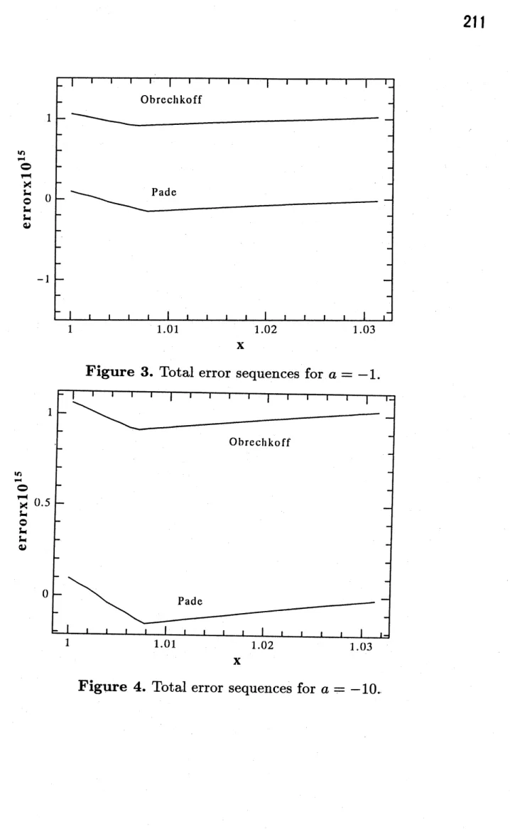
Next we trace the total errors of the two methods in the
cases
thatround-off errors are dominant over the discretization errors. The results
are shown in Fig.3 and 4. The superiority of the method (3.4) is also
clear from the figures. These computations have been performed on an
ACOS 2020 computer of Computer Center of Tohoku University, and the
Figure 1. Total errors at $x=1.03125$ for $a=-1$
.
$-\log_{2}h$
X
Figure 3. Total error sequences for $a=-1$
.
X
4 Concluding remarks
In this paper we have discussed the order barrier of the Adams type
LMM method, and derived some optimal method under the conditions (1.3) and (1.4). However, as discussed in Sec. 3, these conditions are
somewhat restrictive in general situations. It is necessary to discuss the
order barrier and an optimal method under the less restrictive condition
such that
$\beta_{i1}\geq 0,$ $i=0,$ $\cdots,$ $k-1$,
$(-1)^{j-1}\beta_{kj}>0,$ $j=1,$$\cdots,$ $l$,
in which the coefficients $\beta_{ij}$, $(j=2, \cdots , l, i<k)$ are not subject to any
constraints.
References
[1] G. Dahlquist, Convergence and stability in the numerical integration
of ordinary differential equations, Math. Scand., 4(1956), 33-53.
[2] P. J. Davis and P. Rabinowitz, Methods of Numerical Integra-tion, Academic Press, New York, 1975.
[3] G. Hadley, Linear Programming, Addison-Wesley, Reading Mass.,
1978.
[4] E. Hairer, S. P. $N\emptyset rsett$ and G. Wanner, Solving ordinary differential equations I, Nonstiff problems, Springer-Verlag, Berlin,1987.
[5] E. Hairer, G. Wanner, Solvingordinary differential equations II,
Non-stiff problems, Springer-Verlag, Berlin,1991.
[6] R. Jeltsch, Multistep methods using higher derivatives and damping at infinity, Math. of Comp. 31(1977), 124-138.
[7] K. Ozawa, Implicit linear multistep methods with nonnegative
coef-ficients for solving initial value problems, JIP 12(1988), 42-50.
[8] K. Ozawa, Backward differential formulae with nonnegative
coeffi-cients for solving initial value problems, JJIAM 9 $397- 411(1992)$
.
[9] K. Ozawa, Attainable order of Adams type linear multistep
mul-tiderivative method with nonnegative coefficients for solving initial
5 Appendix
Here we will give a conjecture on the order barrier for the linear multistep
method
$y_{n+k}=-\alpha_{k-1}y_{n+k-1}-\cdots-\alpha_{0}y_{n}+h(\beta_{k}f_{n+k}+\cdots+\beta_{0}f_{n})$, (5.1)
where the coefficients $\alpha’ s$ and $\beta’ s$ are subject to the constraints
$-\alpha_{i}\geq 0,$ $i=0,$ $\cdots,$ $k-1$, (5.2)
A
$\geq 0,$ $i=0,$ $\cdots,$ $k$.
(5.3)Wedemand, moreover, theLM method(5.1) to be zero-stable. It is well
known that no zero-stable k-step LM method can have order exceeding
$k+2$, and that if a zero-stable k-step LM method is of order $k+2$ then
the following conditions must be satisfied [1]:
1. The step number $k$ is even.
2. All the zeros ofthe first characteristic polynomial $\rho(\zeta)$, which is given
by
$\rho(\zeta)=\zeta^{k}+\alpha_{k-1}\zeta^{k-1}+\cdots+\alpha_{0}$,
are located on the unit
circle..
3. In particular $\zeta=\pm 1$ are the zeros of $p(\zeta)$
.
It follows, from these conditions, that the characteristic polynomial $\rho(\zeta)$
associated with the method of maximal order has the form
$p( \zeta)=(\zeta^{2}-1)\prod_{\nu}(\zeta^{2}-2\cos\theta_{\nu}\zeta+1)$, (5.4)
and therefore $\alpha_{0}=-1$
.
Moreover the third ofthe above conditions leadsto
implying that
$\alpha_{j}=0,$ $j=1,$ $\cdots,$$k-1$,
since the coefficients $-\alpha’ s$ are nonnegative. We can conclude, from this,
that if the LM method (5.1) with the nonnegative conditions (5.2) and
(5.3) has maximal order$p_{\max}$ then the method must be the Newton-Cotes
type, i.e., the method must be of the form
$y_{n+k}=y_{n+k-1}+h(\beta_{k}f_{n+k}+\cdots+\beta_{0}f_{n})$
.
(5.5)Accordingto Davis and Rabinowitz[2], the coefficients $\beta’ s$of the
Newton-Cotes type formula of order $k+2$, which is equivalent to the Newton-Cotes
type numerical quadrature formula, are given by
$\beta_{i}=\frac{(-1)^{k-i}}{i!(k-i)!}\int_{0}^{k}t(t-1)\cdots(t-i+1)(t-i)\cdots(t-k)dt$,
$i=0,$ $\cdots,$ $k$, (56)
and these coefficients have the asymptotical property
$\beta_{i}=\frac{(-1)^{i-1}k!}{i!(k-i)!k\log^{2}k}[\frac{1}{i}+\cdot\frac{(-1)^{k}}{k-i}][1+O(\frac{1}{\log k})],$ $karrow\infty$
.
(5.7)It can be easily seen from eq.(5.7) that the coefficient $\beta_{i}$ changes its sign
alternatively for sufficiently large $k$
.
Using formula (5.6) we can confirmnumerically that
$\bullet$ For $k=2,4,6$,
$\beta_{i}\geq 0,$ $i=0,$ $\cdots,$ $k$
.
$\bullet$ But for any even $k$ satisfying $8\leq k\leq 20$
$\beta_{\frac{k}{2}}\beta_{\frac{k}{2}-1}<0$
.
Thus, the attainable order $p_{\max}$ of the LM method is expected to be 8, if the coefficients $\alpha’ s$ and $\beta’ s$ are subject to the constraints (5.2) and