37
弱単項二階論理式の例示および反例からの学習
Learning Weak Monadic Second-Order Logical Formulas from Queries and
Counterexamples
東京電機大学理工学部惰報科学科
Department of Information Sciences, Tokyo Denki University
Abstract
Inthis paper, we consider the problem oflearningan unknown weakmonadic
second-order (WMS for short) logical formula from examples making it
true and those making it false. It is well known that, for a WMS formula,
there exists adeterministic frontier-to-root tree automaton (dfrta for short
$)$ accepting the trees which are the encodings of those examples making the
formula true. Thus, we reduce our problem to the problem of learning an
unknown treelanguage from examples of its members and nonmembers. We
assume that the tree language is presented by the Angluin’s minimally
ade-quate teacher, which can answer membership queries and equivalence queries.
Ourlearning algorithm $L_{T}^{*}$ tolearn tree languagesisbased on aslight variant
of the Sakakibara’s polynomial time algorithm to learn deterministic skeletal
automata. The algorithm$L_{T}^{*}$ runsin time polynomial in the number ofstates
ofthe minimum dfrta for the unknown tree language and the maximum size
of any counterexample provided by the teacher. Thus we propose a new
framework of concept learning in which atomic relations such as $”\subseteq$ and
many relations definable by WMS formulas, e.g. prefix-closedness of sets,
can be learned in polynomial time. 数理解析研究所講究録
38
1
Introduction
Inthe theoretical studies of concept learning, the problems oflearningvarious
types oflogical formulas have gained a great deal of attention in recent years.
Many works have been performed in this area. For example, Shapiro showed
an algorithm solving the model inference problem for Horn theories [11]. In
[14], Valiant provided atheoretical basis forlearning boolean formulas. While
Angluin showed a polynomial time $al$gorithm to learn acyclic propositional
Horn sentences using equivalence queries and requests for hints. [2].
In this paper, we consider the problem of learning an unknown weak
monadic second-order (WMS for short) logical formulafrom examples
mak-ing it true and those makmak-ing it false. And we will show a polynomial time
algorithm to learn WMS formulas usingmembership queries and equivalence
queries. Thus we propose a new framework of concept learning in which
atomic relations such as $”\subseteq$ and many relations definable by WMS
formu-las, $e.g$. prefix-closedness of sets, can be learned in polynomial time.
Itisknown that, for a WMS formula, there exists adeterministic
frontier-to-root tree automaton (dfrta for short) accepting the trees which are the
encodings of those examples making the formula true [13]. Thus, we reduce
our problem to the problem of learning an unknown tree language from
ex-amples of its members and nonmembers. We assume that the tree language
is presented by the Angluin’s minimally adequate teacher, which is explained
in the next paragraph.
Concerning the problem oflearning an unknown regular set from
exam-ples, Angluin introduced a learning protocol so called minimally adequate
teacher which can answer membership queries and equivalence queries [1].
Angluin showed that if an unknown regular set is presented by a minimally
adequate teacher, the regular set can be learned in time polynomial in the
number ofstates of the minimum deterministic finite automaton for the
un-known regular set and the maximumlength of any counterexample provided
by the teacher.
In $[9, 10]$, in order to develop an efficient learning algorithm for
context-free grammars, Sakakibara reduced the problem of learning a context-free
grammar from structural data to the problem of learning a deterministic
skeletal automaton, which is a particular kind of dfrta. Then extending the
Angluin’s learning algorithm for finite automata to the one for deterministic
39
grammars. Our learning algorithm $L_{T}^{*}$ to learn dfrtas is based on a slight
variant of this Sakakibara’s polynomial time algorithm. The algorithm $L_{T}^{*}$
runs in time polynomial in the number of states of the minimum dfrta for
the unknown tree language and the maximum size of any counterexample
provided by the teacher.
The paper is organized as follows: In section 2 we review the definition
of tree automata and the related terminol$0$gies. In section 3 we present a
polynonial time algorithm to learn dfrtas which is a slight variant of the
Sakakibara’s polynomial time’algorithm to learn deterministic skeletal
au-tomata. In section 4 we review the definition of weak monadic second-order
theory of multiple successors (WSMS for short) and introduce some
neces-saryterminologies. In section 5 we present our main theorem and illustrate by
two examples how the learner $L_{T}^{*}$ learns a relation definable in the language
associated to the WSMS from queries and counterexamples. We present two
example runs of $L_{T}^{*}$ to learn the unary predicate $PC$ which is the set of
prefix-closed sets, and the binary relation $”\subseteq$ on finite sets.
2
Preliminaries
In this section, we review the definition of tree automata and the related
terminologies. For details, see [9, 12, 13].
An enpty string is denoted by A and the power set of a set $A$ is denoted
by $2^{A}$. For a set $A,$ $A^{*}$ denotes the free monoid generated by $A$. Let $N$ be
the set of non-negative integers. For $x,$ $y\in N,$ $x\succeq y$ iff there exists $z\in N^{*}$
such that $x=yz$, and $x\succ y$ iff$x\succeq y$ and $x\neq y$.
A ranked alphabet is defined to be an pair $V=<\Sigma,$ $\sigma>$, where $\Sigma$ is a
finite set of symbols and $\sigma$ is a napping from $\Sigma$ into $N$. For $a\in\Sigma,$ $\sigma(a)$
is called the rank of $a$. We will denote the set of symbols of rank $n$ by $\Sigma_{n}$,
i.e. $\Sigma_{n}=\sigma^{-1}(n)$. A symbol in the set $\Sigma_{0}$ is called a constant symbol. If we
consider the symbols in $\Sigma_{n}$ as function symbols, the rank of each function
symbol is usually called its arity.
Definition 2.1 A $\Sigma$-tree, or a tree over$\Sigma$ is amapping $t$ from $Dom(t)$ into
$\Sigma$, where $Dom(t)$ is a finite subset of $N^{*}$ satisfying :
40
2. If $yi\in Dom(t)$ for $i\in N$ then $yj\in Dom(t)$ for $j\in N,$ $1\leq j\leq i$.
3. If$t(x)=a\in\Sigma_{n}$ then $xi\in Dom(t)$ for $i\in N,$ $1\leq i\leq n$.
An element of $Dom(t)$ is called a node of $t$. If$t(x)=a$, then $a$ is said to be
the label of the node $x$ of$t$. The set ofall trees over $\Sigma$ is denoted by $T_{\Sigma}$.
Definition 2.2 A ranked alphabet $V=<\Sigma,$ $\sigma>$ uniquely determines a
set Term$(\Sigma)$ of terms over$\Sigma$ defined to be the least subset of$\Sigma^{*}$ satisfying:
1. $\Sigma_{0}\subseteq Term(\Sigma)$.
2. If $f\in\Sigma_{n}$ and $t_{1},$$\ldots,t_{n}\in Term(\Sigma)$ then $ft_{1}\ldots t_{n}\in Term(\Sigma)$.
Since the finite trees over $\Sigma$ can be identified with terms over $\Sigma$, we will
represent trees as terms.
Let $t\in \mathcal{T}_{\Sigma}$. A node$p$in $t$ is a terminalnode iff for all $q\in Dom(t),$ $p\neq q$.
While a node $p$ in $t$ is an interior node iff
$p$ is not a terminal node. The
frontier
of $Dom(t)$ is the set of all terminal nodes in $Dom(t)$. The depth of $p\in Dom(t)$ is the length of$p$ and denoted depth$(p)$. For a tree $t$, we definethe depth of $t$ by depth$(t)= \max\{depth(p)|p\in Dom(t)\}$. For$p\in Dom(t)$,
we define the subtree $t/p$
of
$t$ at$p$ by$t/p(q)=t(pq)$.
Let $ be a new symbol of rank $0$ which is not included in $\Sigma$. Then $\mathcal{T}_{\Sigma}^{\}$
denotes the set of all treesover $\Sigma\cup\{}$ which contains exactly one $-symbol.
For trees $u\in \mathcal{T}_{\Sigma}^{\}$ and $v\in T_{\Sigma}\cup T_{\Sigma}^{\}$, an operation $\#$ to replace the terminal
node labelled $ of $u$ with $v$ is defined as follows :
$u\neq v(p)=\{u(p)v(q)ififp=rq,u(r)=\andq\in Dom(v)p\in Dom(u)andu(p)\neq\,$
For subsets $U\subseteq \mathcal{T}_{\Sigma}^{\}$ and $V\subseteq \mathcal{T}_{\Sigma}\cup \mathcal{T}_{\Sigma}^{\}$, we define $U\neq V=\{u\neq v|u\in U$
and $v\in V$
}.
Definition 2.3 A deterministic
frontier-to-root
tree automata (dfrta forshort) is a quadruple $M=(Q, \Sigma, \delta, F)$ consists of 1-4 as follows :
1. $Q$ is a finite set of states.
2. $\Sigma$ is a ranked alphabet with the maximal rank
41
3. $\delta=(\delta_{0}, \delta_{1}, \ldots, \delta_{n})$ is the state transition function, where
$\delta_{k}$ : $\Sigma_{k}\cross(Q\cup\Sigma_{0})^{k}arrow Q$ $(k=1,2, \ldots, n)$, and
$\delta_{0}(a)=a$ for $a\in\Sigma_{0}$.
4. $F\subseteq Q$ is the set of
final
states.The terminal symbols on the frontier are taken as initial states. We extend
$\delta$ to $\mathcal{T}_{\Sigma}$ as usual by:
$6(ft_{1}\ldots t_{k})=\{\delta_{0}(f,\delta(t_{1}),\ldots,\delta(t_{k}))\delta^{k}(f)$ $ififk=0k>0.$’
A tree $t$ is accepted by $M$ iff$\delta(t)\in F$. We define theset of trees accepted by
$M$ as $L(M)=\{t\in \mathcal{T}_{\Sigma}|\delta(t)\in F\}$. A set $L$ of trees is said to be recognizable
if there exists a dfrta $M$ such that $L=L(M)$.
3
Learning
Tree
Automata
Inthis section, we will present aslight variantof the Sakakibara’s polynomial
timealgorithm to learn deterministic skeletal automata [9] as the one to learn
deterministic frontier-to-root tree automata. For details, see [9].
3.1
Closed
Consistent Observation
Tables
Let $\Sigma$ be a ranked alphabet, $A$ be a finite subset of $\mathcal{T}_{\Sigma}$, and $B$ be a finite
subset of $\mathcal{T}_{\Sigma}^{\}$. A set $A$ is subtree-closed if $a\in A$ then all subtrees with
depth at least 1 of $a$ are included in $A$. While a set $B$ is prefix-closed with
respect to $A$ if $b\in B-\{}$ then there exists a tree $b’\in B$ such that $b=$
$b’\neq fa_{1}\ldots a_{i-1} a_{i}\ldots a_{k-1}$ for some $f\in\Sigma_{k},$ $a_{1},$$\ldots,$$a_{k-1}\in A\cup\Sigma_{0}$ and $i\in N$.
Definition 3.1 An observation table is a 3-tuple $(S, E, T)$ consists of 1-4
as follows :
1. $S$ is a nonempty subtree-closed set of$\Sigma$-trees with depth at least 1.
2. $X(S)=\{fu_{1}\ldots u_{k}|f\in\Sigma_{k},$ $u_{1},$ $\ldots,$$u_{k}\in S\cup\Sigma_{0}$ and $fu_{1}\ldots u_{k}\not\in S$ for
42
3. $E$ is a nonempty finite subset of$\mathcal{T}_{\Sigma}^{\}$ which is prefix-closed with respect
to $S$.
4. $T$ is a finite function mapping $E\neq(S\cup X(S))$ to $\{0,1\}$.
The interpretation of$T$ is as follows : $T(s)=1$ iff$s\in L(M)$ of the unkown
dfrta $M$. An observation table can be visualised as a two-dimensional matrix
with rows labelled by elements of $S\cup X(S)$, columuns labelled by elements
of $E$, and the entry for row $s$ and column $e$ equal to $T(e\# s)$. The learning
algorithm uses the observation table to build a dfrta. If $s$ is an element of
$S\cup X(S),$ $row(s)$ denotes the finite function $g$ from $E$ to $\{0,1\}$ defined by
$g(e)=T(e\# s)$.
An observation table $(S, E, T)$ is closed if every row$(x)$ of $x\in X(S)$ is
identical to some row$(s)$ of $s\in S$. An observation table is called
consis-tent if whenever $s_{1}$ and $s_{2}$ are elements of $S$ such that row$(s_{1})=row(s_{2})$,
row$(fu_{1}\ldots u_{i-1}s_{1}u_{i}\ldots u_{k-1})=row(fu_{1}\ldots u_{i-1}s_{2}u;\ldots u_{k-1})$ for all $f\in\Sigma_{k},$ $u_{1},$ $\ldots$,
$u_{k-1}\in S\cup\Sigma_{0}$ and $1\leq i\leq k$.
Let $(S, E, T)$ be a closed consistent observation table (CCOT for short
$)$. The corresponding
dfrta
$M(S, E, T)$ over $\Sigma$ constructed from $(S, E, T)$ isdefined with thestate set $Q$, the set of final states$F$, and the state transition
function $\delta$ as follows :
$Q=\{row(s)|s\in S\}$,
$F=$
{
$row(s)|s\in S$ and $T(s)=1$},
$\delta_{k}(f, row(s_{1}),$$\ldots,$ $row(s_{k}))=row(fs_{1}\ldots s_{k})$
for $f\in\Sigma_{k}$, and $s_{1},$ $\ldots,$$s_{k}\in S\cup\Sigma_{0}$,
$\delta_{0}(a)=row(a)$ for $a\in\Sigma_{0}$.
The concept of the CCOT was introduced by Angluin [1]. The following
theorem is similarly proved as in [9]
Theorem 3.1 Let$(S, E, T)$ be a CCOT. The
dfrta
$M=M(S, E, T)$defined
above
satisfies
the followingfour
conditions :1. $M$ is
well-defined.
2. For every $s\in S\cup X(S),$ $6(s)=row(s)$.
3. $M$ is consistent with the
finite function
T. That is,for
every $s\in$43
4. Suppose that $M$ has $n$ states.
If
$M’$ is anydfrta
consistent with$T$ thathas$n$ or
fewer
states, then $M’$ is isomorphic to M. $\square$3.2
The
Learning Algorithm
$L_{T}^{*}$Let $L_{U}$ be an unknown recognizable tree language and $M_{U}$ be the minimum
dfrta accepting$L_{U}$. Itis assumedthat the learner knows the ranked alphabet
$\Sigma$ of$M_{U}$. A membership query proposes a $\Sigma$-tree $t$ and asks whether $t\in L_{U}$.
The answer from the teacher is either yes or $no$. While an equivalence query
proposes a dfrta $M$ and asks whether $L(M)=L_{U}$. The answer is either yes
or $no$
.
When the answer is $no$, a counterexample is also provided from theteacher. It is a $\Sigma$-tree $t$ in the symmetric difference of $L_{U}$ and $L(M)$. This
learning protocol is based on Angluin’s “minimally adequate teacher” in [1].
Our algorithm to learn dfrta is shown in Figure 1.
In the algorithm $L_{T}^{*}$, the operation “extend $T$ to $E\#(S\cup X(S))$ using
membership queries” is the operation to extend $T$ by asking membership
queries for missing elements. It is clear that if$L_{T}^{*}$ ever terminates, its output
is adfrta$M$such that $L(M)=L_{U}$. Thefollowing theorem is similarly proved
as in [9]
Theorem 3.2 Let$L_{U}$ be an unknown recognizable tree language and $M_{U}$ be
the minimum
dfrta
accepting $L_{U}$, Using membership and equivalence queriesfor
$L_{Uz}$ the learning algorithm $L_{T}^{*}$ eventually terminates and outputs adfrta
$M$ isomorphic to $M_{U}$ accepting $L_{U}$. Furthermore,
if
$n$ is the numberof
thestates
of
$M_{U}$ and $m$ is the maximum sizeof
any counterexample provided bythe teacher, then the total running time
of
$L_{T}^{*}$ is bounded by a polynomial in$m$ and $n$. $\square$
4
Weak
Monadic
Second-Order Theory of
Multiple Successors
In this section, we review thedefinitionof weak monadicsecond-order theory
of multiple successors (WSMS for short) andintroduce some necessary
ter-minologies. For details, see [13]. We mainly describe how a dfrta recognizes
44
$S:=\Sigma_{0)}\cdot E:=\{};$
Construct the initial observation table $(S, E, T)$ using membership queries
for $al1\Sigma$-trees of depth at most 2; Repeat
While $(S, E, T)$ is not closed or not consistent do
If $(S, E, T)$ is not closed then do
Find $s_{1}\in X(S)$ s.t. row$(s_{1})$ is different from row$(s)$ for all $s\in S$;
Add $s_{1}$ to $S$;
Extend $T$ to $E\neq(S\cup X(S))$ using membership queries
end
If $(S, E, T)$ is not consistent then do
Find $s_{1},$ $s_{2}\in S,$ $e\in E,$ $k\in N,$ $f\in\Sigma_{k},$ $u_{1},$
$\ldots,$
$u_{k-1}\in S\cup\Sigma_{0}$,
and $i\in N$ such that row$(s_{1})=row(s_{2})$ and
$T(e\neq fu_{1}\ldots u_{k-1}s_{1}u_{i}\ldots u_{k-1})\neq T(e\neq fu_{1}\ldots u_{k-1}s_{2}u_{i}\ldots u_{k-1})$;
Add $e\neq fu_{1}\ldots u_{k-1} u;\ldots u_{k-1}$ to $E$;
Extend $T$ to $E\#(S\cup X(S))$ using membership queries
end end
Once $(S, E, T)$ is closed and consistent, let $M$ $:=M(S, E, T)$;
Make the conjecture $M$ using an equivalence query proposing $M$;
If the teacher replies $no$ with a counterexample $t$ then do
Add $t$ and all its subtrees with depth at least 1 to $S$;
Extend $T$ to $E\neq(S\cup X(S))$ using membership queries
end
Until the teacher replies yes to the conjecture $M$;
Halt and output $M$.
45
4.1
A Monadic
Second-Order
Language
$\mathcal{L}_{k}$Let $A_{k}=\{1,2, \ldots, k\}$ be an alphabet. The WSMSs are based on (1) the set
$A_{k}^{*},$ (2) $k$ right-successor functions, $r_{1},$$\ldots,$$r_{k}$, where $r_{i}(w)=wi$ for all $w\in A_{k}^{*}$
and $\lambda i=i(1\leq i\leq k)$, and (3) relations and functions which can be defined
recursively from the
successor
functions of (2). In this paper, we deal withthe weak monadic second-order theory
of
$A_{k}^{*}$ with the $k$ successorfunctions.
The associated language $\mathcal{L}_{k}$ is a monadic second-order language consisting
of the following :
$\bullet$ individual variables, $x,$
$y,$$z,$$x_{1},$ $y_{1},$$z_{1},$$\ldots$, ranging over $A_{k}^{*}$
.
$\bullet$ set variables, $\alpha,$$\beta,$$\alpha_{1},$$\beta_{1},$$\ldots$, ranging over finite subsets of$A_{k}^{*}$. $\bullet$ constants
$=,$ $\in with$ their usual interpretation.
$\bullet$ binary predicate symbols $R_{i},$ $i\in A_{k}$ interpreted as follows: $R_{t}(u, v)rightarrow$
$r_{i}(u)=vrightarrow ui=v$.
$\bullet$ propositional connectives $A_{\rangle}\neg$ ; individualquantifier, $\exists$ ; set quantifier, $\exists$ ; punctuation and parentheses.
Notice that $\vee,$ $\forall andarrow can$ be defined $using\wedge,$ $\neg$ and $\exists$
.
So, in the sequel,we also use $\vee,$ $\forall andarrow to$ define relations in $\mathcal{L}_{k}$. Atomic
formulas
are thoseexpressions of the form $x=y,$ $x\in\alpha$ or $R_{i}(x, y)$.
Definition 4.1 $\mathcal{L}_{k}$
-formulas
are recursively defined as follows:1. Atomic formulas are $\mathcal{L}_{k}$-formulas.
2. If $F$ and $G$ are $\mathcal{L}_{k}$-formulas, then $F\wedge G,$ $\neg F,$ $\exists xF$ and $\exists\alpha F$ are all
$\mathcal{L}_{k}$-formulas.
3. Nothing other than those that can be defined by means of a finite
number of applications of the rules 1 and 2 are $\mathcal{L}_{k}$-formulas.
The sentences of $\mathcal{L}_{k}$ are those $\mathcal{L}_{k}$-formulas including no free variables. The
46
Example 4.1 Let $PC(\alpha)$ be a unary predicate which is the set of
prefix-closed subsets of $A_{2}^{*}$. That is, $PC(\alpha)$ is true iff a set $\alpha$ is prefix-closed.
$PC(\alpha)$ is definable in $\mathcal{L}_{2}$ :
$PC(\alpha)^{def}rightarrow\forall x([\exists y(R_{1}(x, y)\wedge y\in\alpha)\vee\exists y(R_{2}(x, y)\wedge y\in\alpha)]arrow(x\in\alpha))$ .
The weak monadic second-order theory ofone successor (the case $k=1$
$)$ is known to be decidable [3, 4, 7], that is, there is an effective procedure
for deciding truth of sentences of$\mathcal{L}_{1}$. While, the weak monadic second-order
theory of multiple successors is also shown to be decidable using concepts of
generalized finite automata, which is equivalent to dfrta [4, 5, 13]. That is,
the following theorem is known:
Theorem 4.1 [5] The weak monadic second-order theory
of
multiplesuc-cessors is decidable. $\square$
4.2
Recognizing
Definable Relations
of
$\mathcal{L}_{2}$In the sequel, we will concentrate the case $k=2$ because the genaralization
for more than two successor functions offers no difficulty. The outline of the
procedure to recognize a definable relation of the language $\mathcal{L}_{2}$ is as follows :
1. Find a language $\mathcal{L}_{2}’$ equivalent to $\mathcal{L}_{2}$ which involvesno individual
vari-ables or individual quantifiers.
2. Encode n-tuples of finite subsets of$A_{2}^{*}$ asterms on the ranked alphabet
$\Sigma^{n}=\Sigma_{0}^{n}\cup\Sigma_{2}^{n}$, where $\Sigma_{0}^{n}=\{\epsilon\}$ and $\Sigma_{2}^{n}=\{0,1\}^{n}$.
3. Find adfrtarecognizingevery definable relation of$\mathcal{L}_{2}’$interpreted under
the encoding of 2 (Existence of such a dfrtais guaranteed by theorem
4.2 stated in below).
Now we will describe the equivalent language $\mathcal{L}_{2}’$ and theencoding of n-tuples
of finite subsets of$A_{2}^{*}$.
The equivalent Language $\mathcal{L}_{2}’$
The individual variables of$\mathcal{L}_{2}$ can be eliminated by simplyreplacing them
47
set variables in one-one correspondence with the individual variables. The
language $\mathcal{L}_{2}’$ is a monadic second-order language consisting of the following:
$\bullet$ set variables, $\alpha_{x},$$\alpha_{y},$$\alpha_{z},$ $\alpha_{x_{1}},$$\alpha_{y_{1}},$$\alpha_{z_{1}},$ $\ldots$, ranging over singleton subsets
of $A_{2}^{*}$.
$\bullet$ set variables, $\alpha,$$\beta,$$\alpha_{1},$ $\beta_{1},$
$\ldots$, ranging over finite subsets of$A_{2}^{*}$. $\bullet$ $constant\subseteq$ with its usual interpretation.
$\bullet$ binary predicate symbols $\overline{R}_{i},$
$i\in A_{i}$ interpreted as follows: $\overline{R}_{i}(\alpha, \beta)rightarrow$
$\alpha$ and $\beta$ are singletons and $\hat{r}_{i}(\alpha)=\beta(\hat{r}_{i}$ is the set function induced
by $r_{i}$ ).
$\bullet$ propositional connectives $\wedge,$ $\neg$ ; set quantifier, $\exists$ ; punctuation and
parentheses.
The formation rules for $\mathcal{L}_{2}’$ arelike those of$\mathcal{L}_{2}$ except that individual variables
are not involved.
Next we define a translation $\tau$ from $\mathcal{L}_{2}$ to $\mathcal{L}_{2}’$. Weintroduce the predicate
SI$(\alpha)$ which is the set ofsingleton subsets. $SI$ is definable in $\mathcal{L}_{2}’$ :
SI$(\alpha)$ def $\forall\beta[\beta\supseteq\alphaarrow(\alpha\supseteq\beta$ $\vee$ $\forall\beta_{1}(\beta\supseteq\beta_{1}))]$ $\wedge$ $\exists\beta_{1}(\neg\alpha\supseteq\beta_{1})$.
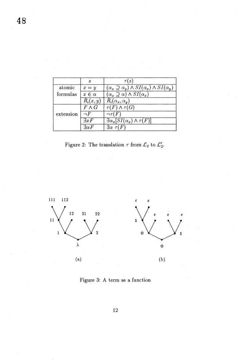
Then the translation is defined as shown in Figure 2. It should be clear that
if $s$ is anysentence in $\mathcal{L}_{2}$ then $s$ is true iff $\tau(s)$ is true.
The encoding
of finite
subsetsof
$A_{2}^{*}$Here, we will be working with the ranked alphabet $\Sigma^{1}=\Sigma_{0}^{1}\cup\Sigma_{2}^{1}$, where $\Sigma_{0}^{1}=\{\epsilon\}$ and $\Sigma_{2}^{1}=\{0,1\}$. We define terms as functions from finite
pre-fix closed subsets of $A_{2}^{*}$ into $\Sigma^{1}$. For example, the term $t=001\epsilon\epsilon\epsilon 1\epsilon\epsilon$
shown in Figure 3 (b) corresponds to the function from a set $S=\{\lambda,$ $1,2,11$,
12, 21, 22, 111,
112}
into$\Sigma^{1}$ definedby the correspondingposition of the treesin Figure 3, e.g. $t(\lambda)=0,$ $t(11)=1,$ $t(112)=\epsilon$.
If we look at the inverse image of some function symbol, we are able to
associate a finite subset of$A_{2}^{*}$ with a term. For example, as can be seen from
48
Figure 2: The translation $\tau$ from $\mathcal{L}_{2}$ to $\mathcal{L}_{2}’$.
111 112 $e$ $e$
$\lambda$
$0$
(a) (b)
49
Thus, a term in $T_{\Sigma 1}$ can be viewed as acharacteristic function of afinite
subset of $A_{2}^{*}$, that is, the set associated with such a term $t$ is $t^{-1}(1)$. An
inductive definition of the mapping $c$ which assigns to each $t\in\tau_{\Sigma^{1}}$ a finite
subset $c(t)\subseteq A*$ is as follows :
1. $c(\epsilon)=\emptyset$,
2. $c(0t_{1}t_{2})=l_{1}c(t_{1})\wedge\wedge\cup l_{2}^{\wedge}c(t_{2})\wedge$
$c(1t_{1}t_{2})=l_{1}c(t_{1})\cup l_{2}c(t_{2})\cup\{\lambda\}$,
where $l_{i}$ is the left successor by the symbol $i$, i.e. $l_{i}(w)=iw$, and $l_{i}^{\wedge}$
is the set function induced by $l_{i}$.
It is inductively proved that the function $c$ is onto $2^{A_{2}^{*}}$. Though, $c$ is not
one-one. In general, $c(t)=c(t’)$ iff $t$ and $t$‘ differ only by subterms in the
function symbol $0$. Thus, we define the encoding $e(\alpha)$ of $\alpha$ to be the term in
$c^{-1}(\alpha)$ in which $0\epsilon\epsilon$is not a subterm. The following proposition is known:
Proposition 4.1 [13] The set
of
encodingsof finite
subsetsof
$A_{2}^{*}$ isrecog-nizable. $\square$
The encoding
of
n-tuplesof finite
subsetsof
$A_{2}^{*}$We now define the encoding of n-tuples offinite sets. We will be working
with the ranked alphabet $\Sigma^{n}=\Sigma_{0}^{n}\cup\Sigma_{2}^{n}$, where $\Sigma_{0}^{n}=\{\epsilon\}$ and $\Sigma_{2}^{n}=\{0,1\}^{n}$. Define the mapping $p_{i}$ : $\{0,1\}^{n}arrow\{0,1\}(i=1, \ldots, n)$ by $p_{i}(a_{1}, \ldots, a_{n})=a_{l}\cdot$.
Then, we extend $p_{i}$ to aprojection$\overline{p}_{\dot{l}}$ : $T_{\Sigma^{n}}arrow T_{\Sigma 1}$. Wefirst define amapping
$c_{n}$ from $T_{\Sigma^{n}}$ to $(2^{A_{2}^{*}})^{n}$ by
$c_{n}(t)=(c\overline{p}_{1}t, \ldots, c\overline{p}_{n}t)$.
Again, the encoding of an n-tuple $\overline{\alpha}=(\alpha_{1}, \ldots, \alpha_{n})$ is chosen to be the term
$e(\overline{\alpha})$ in $c_{n}^{-1}(\overline{\alpha})$ in which $0\ldots 0\epsilon\epsilon$ is not a subterm. For example, a term in
Figure 4 is equal to $e(\{\lambda, 1,11\}, \{1,21\})$. The following proposition is known
:
Proposition 4.2 [13] The set
of
encodingsof
n-tuplesof finite
subsetsof
$A_{2}^{*}$ is recognizable. $\square$
5
{)
$\epsilon$ $\epsilon$ $\epsilon$ $\epsilon$
10
Figure 4: An encoding of a pair of finite sets.
iff $\hat{e}R$ is arecognizable tree language, where $\hat{e}$ is the set function induced by
$e$. The following theorem is known :
Theorem 4.2 [13]
If
$R$ is a relationdefinable
in $\mathcal{L}_{2}’$ then $R$ is recognizable. $\square$5
Learning
Weak
Monadic
Second-Order
Log-ical Formulas
In this section, we present our main theorem concerning the learning of a
relation definable in $\mathcal{L}_{k}$. Then weillustrate by two examples how the learner
$L_{T}^{*}$ learns a relation definable in $\mathcal{L}_{2}$ from queries and counterexamples.
5.1
Main
Theorem
Immediately from theorems 3.2 and 4.2, we obtain the following main
theo-rem:
Theorem 5.1 Let $R$ be a relation
definable
in $\mathcal{L}_{k}$ and $M_{R}$ be the minimumdfrta
accepting $\hat{e}R$. Using membership and equivalence queriesfor
$\hat{e}R$, thelearning algorithm $L_{T}^{*}$ eventually terminates and outputs a
dfrta
$M$isomor-phic to $M_{R}$ accepting $\hat{e}R$. Furthermore,
if
$n$ is the numberof
the statesof
$M_{R}$and $m$ is the maximum size
of
any counterexample provided by the teacher,$5j_{-}$
Corollary 5.1 Let $R$ be a relation
definable
in $\mathcal{L}_{k}$. There is an algorithmto learn $R$ using membership and equivalence queries that runs in time
poly-nomial in the number
of
statesof
the minimumdfrta
accepting $\hat{e}R$ and themaximum length
of
any counterexample provided by the teacher. $\square$We assume that the learner $L_{T}^{*}$ knows the following things :
1. the ranked alphabet of the dfrta to be learned,
2. the valid encoding of finite subsets of$A_{k}^{*}$.
Thus, for a term $t$ which is not a valid encoding for any tuple of finite
subsets of$A_{k}$ (i.e. $t$ has $0\ldots 0ee$ as a subterm), $L_{T}^{*}$ automatically fills in the
corresponding entry ofthe observation table with “$0$’ without asking to the
teacher.
5.2
Two Examples
In this subsection, we will illustrate by two examples how the learner $L_{T}^{*}$
learns a relation definable in $\mathcal{L}_{2}$ from queries and counterexamples. In
exam-ples 5.1 and 5.2, we present example runs of $L_{T}^{*}$ to learn the unary predicate
$PC$ of Example 4.1 and the binary relation $”\subseteq$ , respectively.
Example 5.1 (Learning of the unary predicate $PC$ of Example 4.1)
As mentioned above, we assume that the learner $L_{T}^{*}$ knows the ranked
alphabet $\Sigma^{1}=(\Sigma_{0}^{1}, \Sigma_{2}^{1})$, where $\Sigma_{0}^{1}=\{e\}$ and $\Sigma_{2}^{1}=\{0,1\}$. It is easy to see
that
$L_{PC}=\{t\in T_{\Sigma^{1}}|t=e(\alpha)$ for some $\alpha\subseteq A_{2}^{*}$, and if $v\prec u$ and $t(u)=1$
then $t(v)=1.$
}
is the unknown recognizable tree languag$e$ to be learned.
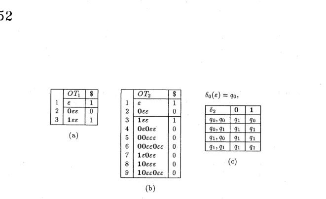
The learner $L_{T}^{*}$ constructs the initial observation table $OT_{1}$ shown in
Figure 5 (a) using membership queries for all $\Sigma^{1}$-trees with depth at most 2.
Since Oee is an invalid encoding, $L_{T}^{*}$ automatically fills in the entry in the
row 2 of $OT_{1}$ with $0$’ as mentioned above. In order to fill in the entries in
52
$OT_{1}$ $ $OT_{2}$ $ $5_{0}(e)=q_{0}$,
1 $\epsilon$ 1 1 $e$ 1 2 $0ee$ $0$ 2 $Oee$ $0$ 3 lee 1 3 lee 1 4 OeOee $0$ (a)5 $00eee$ $0$ 6 $O0e\epsilon Oee$ $0$ 7leOee $0$ 8 lOeee $0$ (c) 9 $10eeOee$ $0$ (b)
Figure 5: The learning of the predicate $PC,$ $(a)OT_{1},$ $S=\{\epsilon\},$ $E=\{},$ (b)
$OT_{2},$ $S=\{e, 0e\epsilon\},$ $E=\{},$ (c) the conjecture $M$ of $L_{T}^{*}$.
$L_{PC}$ ?” and “$1\epsilon\epsilon\in L_{PC}$ ?”, respectively. Each of these queries respectively
corresponds to asking “$\emptyset$ is prefix-closed ?” and “
$\{\lambda\}$ is prefix-closed ?”.
Since $OT_{1}$ is not closed, $L_{T}^{*}$ adds $0\epsilon e$ to $S$ and construct the second
observation table $OT_{2}$ shown in Figure 5 (b) by extending $OT_{1}$. Notice that
when $L_{T}^{*}$ constructs $OT_{2}$ from $OT_{1},$ $L_{T}^{*}$ does not propose any membership
query to the teacher. This is because every term in the rows from 4 to 9
of $OT_{2}$ has Oee as a subterm and thus they are invalid encodings. Hence,
$L_{T}^{*}$ automatically fills in the entries in the rows from 4 to 9 with $0’$. Since
$OT_{2}$ is a CCOT, $L_{T}^{*}$ makes the first conjecture $M$ presented in Figure 5 (c)
and proposes an equivalence query, The initial state of $M$ is $q_{0}$ and the final
state is also $q_{0}$. Since $M$ is a correct dfrta for $L_{PC}$, the teacher replies to this
conjecture with yes. Thus, $L_{T}^{*}$ halts and outputs $M$.
The total number of membership queries during this example run is 2 $($
$L_{T}^{*}$ asked to the teacher only about rows 1 and 3 of $OT_{1}$ ). And $L_{T}^{*}$ makes 1
correct conjecture only.
Example 5.2 (Learning of the binary relation $”\subseteq$ )
We assume that the learner $L_{T}^{*}$ knows the ranked alphabet $\Sigma^{2}=(\Sigma_{0}^{2}, \Sigma_{2}^{2})$,
where $\Sigma_{0}^{2}=\{\epsilon\}$ and $\Sigma_{2}^{2}=\{00,01,10,11\}$. Notice that in this example, $e$ is
not a valid encoding for any pair of finite subsets of $A_{2}^{*}$. It can be seen that
53
labelled by
10.}
is the unknown recognizable tree language to be learned.
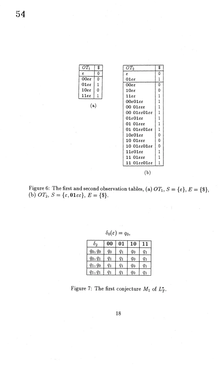
Thelearner constructs the initial observation table $OT_{1}$ shown in Figure
6 (a) using membership queries for all $\Sigma^{2}$-trees with depth at most 2. Since
$OT_{1}$ is not closed, $L_{T}^{*}$ adds Olee to $S$ and construct the second observation
table $OT_{2}$ shown in Figure 6 (b) by extending $OT_{1}$. Since $OT_{2}$ is a CCOT,
$L_{T}^{*}$ makes the first conjecture $M_{1}$ presented in Figure 7. The initial state of
$M_{1}$ is $q_{0}$ and the final state $i_{S}^{\backslash }q_{1}$.
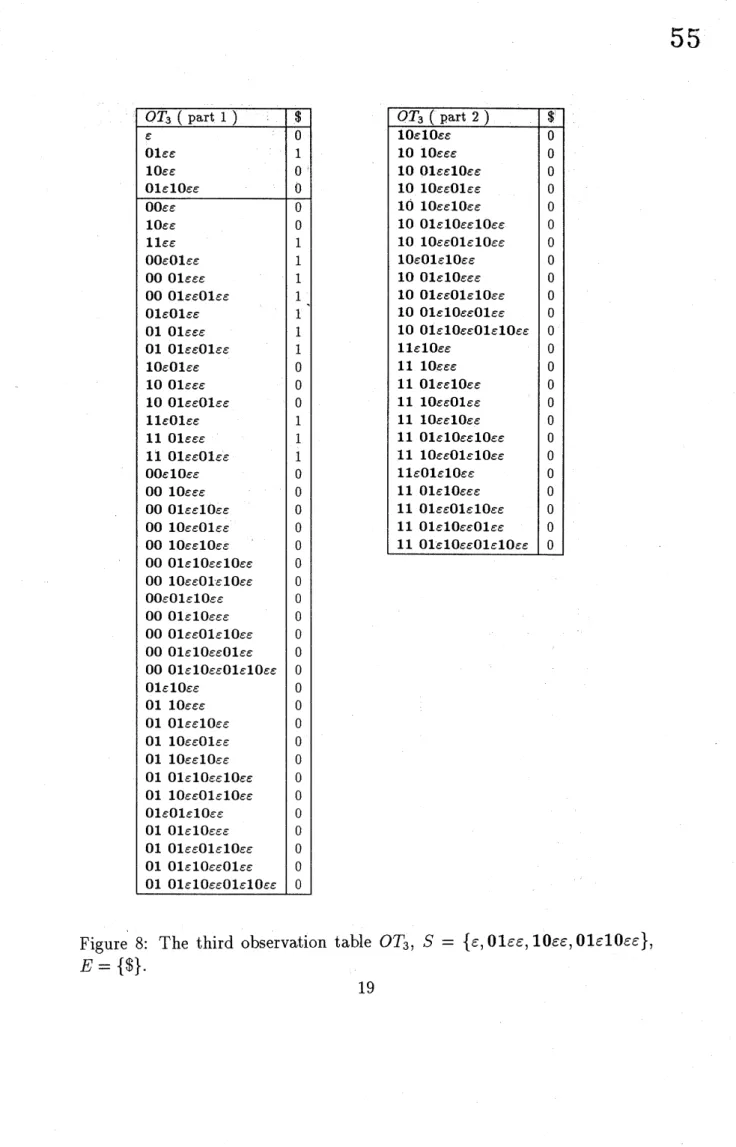
Since $M_{1}$ is notacorrect dfrta for $L_{SUB}$, the teacher replies to this
conjec-ture with $no$ and provides a counterexample. Let us assume that the teacher
provides the counterexample $01e10\epsilon e$. It is not in $L_{SUB}$ but accepted by $M_{1}$.
Then, $L_{T}$ adds the counterexample and all its subtrees to $S$ and constructs
the third observation table $OT_{3}$ in Figure 8 by extending $OT_{2}$.
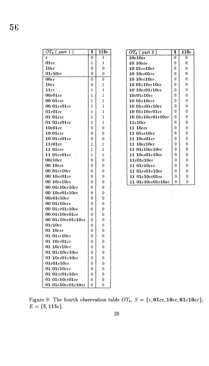
This time $OT_{3}$ is closed but is not consistent. So, $L_{T}^{*}$ adds 11$\epsilon to $E$ and
construct the fourth observation table $OT_{4}$ shown in Figure 9 by extending
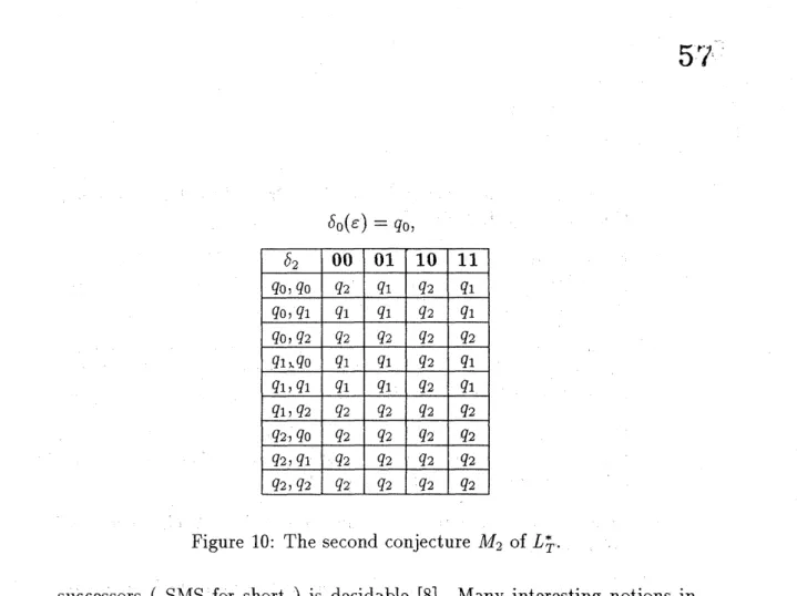
$OT_{3}$. Since $OT_{4}$ is a CCOT, $L_{T}^{*}$ makes the second conjecture $M_{2}$ shown in
Figure 10. The initial state of $M_{2}$ is
$q_{0}$ and the final state is $q_{1}$. Since $M_{2}$
is a correct dfrta for $L_{SUB}$, the teacher replies to this conjecture with yes.
Thus, $L_{T}^{*}$ halts and outputs $M_{2}$.
The toatl number of membership queries during this example run is 130.
And $L_{T}^{*}$ makes 1 incorrect conjecture and 1 correct conjecture.
6
Concluding
Remarks
In this paper, we have shown that weak monadic second-order logical
formu-las can be learned in polynomial time using membership queries and
equiv-alence queries. Since the learner $L_{T}^{*}$ knows the valid encodings of finite sets,
the number of membership queries used by $L_{T}^{*}$ becomes very small in some
cases such as in Example 4.1. Though, it is still an open problem to
substan-tially reduce the number of membership queries used by $L_{T}^{*}$. On the other
hand, the numbers of equivalence queries used by $L_{T}^{*}$ in Examples 5.1 and
5.2 are both quite small compared with the cases in the Shapiro’s framework
[11].
There is an interesting and important extension of our framework to be
54
(a)
(b)
Figure 6: The first and secondobservationtables, (a) $OT_{1},$ $S=\{e\},$ $E=\{},$
(b) $OT_{2},$ $S=\{e, 01ee\},$ $E=\{}.$
$\delta_{0}(\epsilon)=q_{0}$,
55
56
Figure 9: The fourth observation table $OT_{4},$ $S=$
{
$,$Olee,
$10e\epsilon,$ $01\epsilon 10e\epsilon$
},
$E=${
$\,$ll$s}.
$5^{r}1^{4}$
$6_{0}(\epsilon)=q_{0}$,
Figure 10: The second conjecture $M_{2}$ of$L_{T}^{*}$
.
successors (SMS for short) is decidable [8]. Many interesting notions in
various fields of mathematics such as topology and Boolean algebra can be
defined in SMS. So, it is to be expected that a polynomial time algorithm to
learn SMS formula may be developed. But in order to achive this, a
poly-nomial time algorithm to learn rv-tree automata is needed because Rabin’s
decidability results are based
on
the recognition problem of tree automataoninfinite trees. This is the subject for the further research.
Acknowledgments
The author would like to express his sincere thanks to Professor Hiroshi
Noguchi of Waseda University for his kind advice. He also thanks Professors
Takeo Yaku and Akeo Adachi of Tokyo Denki University for their valuable
suggestions.
References
[1] Angluin, D. :“Learning Regular Sets from Queries and
58
[2] Angluin, D. :“Learning with Hints”, in Proc. of the First Workshop on
Computational Learning Theory, Morgan Kaufmann (1988).
[3] B\"uchi, J. R., and Elgot, C. C. : “Decision Problems of Weak Second
Order Arithmetics and Finite Automata”, Abstract 553-112, Notices
Amer. Math. Soc. 5 (1958), p.834.
[4] B\"uchi, J. R. : ) Weak Second-Order Arithmetics and Finite Automata”,
University of Michigan, Logic of Computers Group Techinical Report,
September 1959; Z. Math. Logik Grundlagen Math. 6 (1960), pp.66-92.
[5] Doner, J. E. :“Decidability ofthe Weak Second Order Theory of Two
Successors”, Abstract 65T-468, Notices Amer. Math. Soc. 12 (1965),
p.819 ; erratum, ibid. 13 (1966), p.513.
[6] Doner, J. E. :“Tree Acceptors and Some of Their Applications”, JCSS,
Vol.4 (1970), pp.406-451.
[7] Elgot, C. C. :“Decision Problems of Finite Automata Design and
Re-lated Arithmetics”, Trans. Amer. Math. Soc., Vol.98 (1961), pp.21-51. [8] Rabin, M. O. :“Decidability of Second-Order Theories and Automata
on Infinite Trees”, Trans. Amer. Math. Soc., Vo1.141 (1969), pp.1-35.
[9] Sakakibara, Y. : “Learning Context-Free Grammars from Structural
Data in Polynomial Time”, in Proc. of the First Workshop on
Compu-tational Learning Theory, Morgan Kaufmann (1988).
[10] Sakakibara, Y. :“An Efficient Learning of Context-Free Grammars for
Bottom-Up Parsers”, in Proc. of FGCS’88 (1988).
[11] Shapiro, E. : “Inductive Inference of Theories From Facts”, Research
Report 192, Yale University, Department of Computer Science (1981).
[12] Thatcher, J. W. :“Tree Automata: An Informal Survey” in Aho, A.
V., Ed., Currents in the Theory
of
Computing, Prentice-Hall (1973).[13] Thatcher, J. W. and Wright, J. B. : “Generarized Finite Automata
Theory with an Application to a Decision Problem of Second-Order