Considerations on Fairness-aware Data Mining
Toshihiro Kamishima∗,Shotaro Akaho∗, Hideki Asoh∗, and Jun Sakuma†
∗National Institute of Advanced Industrial Science and Technology (AIST), AIST Tsukuba Central 2, Umezono 1-1-1, Tsukuba, Ibaraki, 305-8568 Japan,
Email: [email protected] (http://www.kamishima.net/), [email protected], and [email protected]
†University of Tsukuba; and Japan Science and Technology Agency;
1-1-1 Tennodai, Tsukuba, 305-8577 Japan; and 4-1-8, Honcho, Kawaguchi, Saitama, 332-0012 Japan Email: [email protected]
Abstract—With the spread of data mining technologies and the accumulation of social data, such technologies and data are being used for determinations that seriously affect individuals’ lives. For example, credit scoring is frequently determined based on the records of past credit data together with statistical prediction techniques. Needless to say, such determinations must be nondiscriminatory and fair regarding sensitive features such as race, gender, religion, and so on.
Several researchers have recently begun to develop fairness- aware or discrimination-aware data mining techniques that take into account issues of social fairness, discrimination, and neutrality. In this paper, after demonstrating the applications of these techniques, we explore the formal concepts of fairness and techniques for handling fairness in data mining. We then provide an integrated view of these concepts based on statistical independence. Finally, we discuss the relations between fairness-aware data mining and other research topics, such as privacy-preserving data mining or causal inference.
Keywords-fairness, discrimination, privacy I. INTRODUCTION
In this paper, we outline analysis techniques of fairness- aware data mining. After reviewing concepts or techniques for fairness-aware data mining, we discuss the relations between these concepts and the relations between fairness- aware data mining and other research topics, such as privacy- preserving data mining and causal inference.
The goal of fairness-aware data mining is for data-analysis methods to take into account issues or potential issues of fairness, discrimination, neutrality, and independence.
Techniques toward that end were firstly developed to avoid unfair treatment in serious determinations. For example, when credit scoring is determined, sensitive factors, such as race and gender, may need to be deliberately excluded from these calculations. Fairness-awareness data mining techniques can be used for purposes other than avoiding unfair treatment. For example, they can enhance neutrality in recommendations or achieve data analysis that is inde- pendent of information restricted by laws or regulations.
Note that in a previous work, the use of a learning algorithm designed to be aware of social discrimination was calleddiscrimination-aware data mining. However, we hereafter use the terms, “unfairness” / “unfair” instead of
“discrimination” / “discriminatory” for two reasons. First, as described above, these technologies can be used for var- ious purposes other than avoiding discriminatory treatment.
Second, because the termdiscrimination is frequently used for the meaning of classification in the data mining literature, using this term becomes highly confusing.
After demonstrating applications tasks of fairness-aware data mining in section II and defining notations in section III, we review the concepts and techniques of fairness-aware data mining in section IV and discuss the relations between these concepts in section V. In section VI, we show how fairness-aware data mining is related to other research topics in data mining, such as privacy-preserving data mining and causal inference. Finally, we summarize our conclusions in section VII.
II. APPLICATIONS OFFAIRNESS-AWAREDATAMINING
Here we demonstrate applications of mining techniques that address issues of fairness, discrimination, neutrality, and/or independence.
A. Determinations that are Aware of Socially Unfair Factors Fairness-aware data mining techniques were firstly pro- posed for the purpose of eliminating socially unfair treat- ment [1]. Data mining techniques are being increasingly used for serious determinations such as credit, insurance rates, employment applications, and so on. Their emergence has been made possible by the accumulation of vast stores of digitized personal data, such as demographic information, financial transactions, communication logs, tax payments, and so on. Needless to say, such serious determinations must guarantee fairness from both the social and legal viewpoints;
that is, they must be fair and nondiscriminatory in relation to sensitive features such as gender, religion, race, ethnicity, handicaps, political convictions, and so on. Thus, sensitive features must be carefully treated in the processes and algorithms of data mining.
According to the reports of existing work, the simple elimination of sensitive features from calculations is insuf- ficient for avoiding inappropriate determination processes, due to the indirect influence of sensitive information. For 2012 IEEE 12th International Conference on Data Mining Workshops
2012 IEEE 12th International Conference on Data Mining Workshops
example, when determining credit scoring, the feature of raceis not used. However, if people of a specific race live in a specific area andaddressis used as a feature for training a prediction model, the trained model might make unfair determinations even though theracefeature is not explicitly used. Such a phenomenon is called a red-lining effect [2] or indirect discrimination [1]. Worse, avoiding the correlations with sensitive information is becoming harder, because such sensitive information can be predicted by combining many pieces of personal information. For example, users’ demo- graphics can be predicted from the query logs of search en- gines [3]. Click logs of Web advertisements have been used to predict visitors demographics, and this information was exploited for deciding how customers would be treated [4].
Even in such cases that many factors are complexly compos- ited, mining techniques must be demonstrably fair in their treatment of individuals.
B. Information Neutral Recommendation
Techniques of fairness-aware data mining can be used for making recommendations while maintaining neutrality regarding particular viewpoints specified by users.
The filter bubble problem is the concern that personaliza- tion technologies, including recommender systems, narrow and bias the topics of information provided to people, unbeknownst to them [5]. Pariser gave the example that politically conservative people are excluded from his Face- book friend recommendation list [6]. Pariser’s claims can be summarized as follows. Users lose opportunities to obtain information about a wide variety of topics; the individual obtains information that is too personalized, and thus the amount of shared information in our society is decreased.
RecSys 2011, which is a conference on recommender systems, held a panel discussion focused on this filter bubble problem [7]. Because selecting specific information by def- inition leads to ignoring other information, the diversity of users’ experiences intrinsically has a trade-off relation to the fitness of information for users’ interests, and it is infeasible to make absolutely neutral recommendation. However, it is possible to make an information neutral recommendation [8], which is neutral from a specific viewpoint instead of all viewpoints. In the case of Parisers Facebook example, a system could enhance the neutrality of political view- point, so that recommended friends could be conservative or progressive, while the system continues to make biased decisions in terms of other viewpoints, for example, the birthplace or age of friends. Thus, techniques of fairness- aware data mining can be used for enhancing neutrality in recommendations.
C. Non-Redundant Clustering
We give an example of the use of clustering algorithm that can deal with the independence from specified information, which was developed before the proposal of fairness-aware
data mining. Coordinated Conditional Information Bottle- neck (CCIB) [9] is a method that can acquire clusterings that are statistically independent from a specified type of information. This method was used for clustering facial images. Simple clustering methods found two clusters: one contained only faces, and the other contained faces with shoulders. If this clustering result is useless for a data analyzer, the CCIB could be used for finding more useful clusters that are composed of male and female images, independent of the useless information. As in this example, techniques of fairness-aware data mining can be used to exclude useless information.
III. NOTATIONS
We define notations for the formalization of fairness- aware data mining. Random variables,SandX, respectively denote sensitive and non-sensitive features. Techniques of fairness-aware data mining maintain fairness regarding the information expressed by this sensitive feature. In the case of discrimination-aware data mining (section II-A), the sen- sitive feature may regard gender, religion, race, or some other feature specified from social or legal viewpoints. In the case of information neutral recommendation (section II-B), a sensitive feature corresponds to a users specified viewpoint, such as political convictions in the example from Pariser.
In an example of non-redundant clustering (section II-C), useless information is expressed as a sensitive feature. S can be discrete or continuous, but it is generally a binary variable whose domain is {+,−} in existing researches.
Individuals whose sensitive feature takes values of+and− are in anunprotectedstate and aprotectedstate, respectively.
The group of all individuals who are in a protected state is a protected group, and the rest of individuals comprise an unprotected group. Non-sensitive features consist of all features other than sensitive features. Xis composed of K random variables, X(1), . . . , X(K), each of which can be discrete or continuous.
Random variableY denotes atarget variable, which ex- presses the information in which data analysts are interested.
If Y expresses a binary determination in a discrimination- aware data mining case, the advantageous class corresponds to the positive class, +, while − indicates the disadvanta- geous class. In an implementation of an information neutral recommender system in [8], Y is a continuous variable representing preferential scores of items.
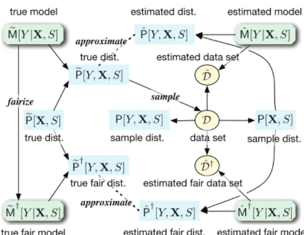
An individual is represented by a pair of instances, x and s, of variables, X and S. A (normal) true model, M[ Y|X, S], is used for determining the instance value of a target variable,Y, for an individual represented byxand s. Because this determination process is probabilistic, this true model corresponds to a conditional distribution of Y given X and S. M[Yˆ |X, S] denotes a (normal) estimated model of this true model. A true fair model, M†[Y|X, S], is a true model modified so that the fairness of the target
P[Y,X, S]
P[ˆY,X, S]
Pˆ†[Y,X, S] P†[Y,X, S]
P[Y,X, S]
P[X, S] P[X, S]
M[Y|X, S]
M†[Y|X, S] Mˆ†[Y|X, S]
M[ˆ Y|X, S]
D Dˆ
Dˆ†
fairize sample
approximate
approximate true model
true fair model
estimated model
estimated fair model true fair dist.
true dist.
true dist.
estimated dist.
estimated fair dist.
sample dist. data set sample dist.
estimated fair data set estimated data set
Figure 1. A summary of notations of models and distributions
variable is enhanced. We call an estimated model of this true fair model by theestimated fair model,Mˆ†[Y|X, S].
Instances x and s are generated according to the true distribution of X and S, P[X, S], and an instance, y, is sampled from a distribution represented by the true model, M[ Y|X, S]. A joint distribution obtained by this genera- tive process is denoted by P[Y,X, S]. A data set, D = {(yi,xi, si)}, i= 1, . . . , N, is generated by repeating this process N times. P[Y,X, S] denotes a sample distribution observed over this data set.
Estimated value yˆ is obtained by applying (xi, si)∈ D to an estimated model, M[ˆ Y|X, S], and a triple (ˆy,x, s) is generated. This process is repeated for all data in D, and we get an estimated data set,Dˆ. Anestimated sample distributioninduced from a sample distribution and an esti- mated model is denoted byP[ˆY,X, S]. The marginalized and conditioned distributions of these three types of distributions, P[Y,X, Y],P[Y,X, Y], andP[ˆ Y,X, Y], are represented by the same symbols. A true fair distribution, a sample fair distribution, and an estimated fair distributionare obtained by substituting normal models, M[·] and M[·]ˆ , with fair models,M†[·]andMˆ†[·], and these are represented byP†[·], P†[·], andPˆ†[·], respectively. Anestimated fair data set,Dˆ†, is generated by a similar generative process of an estimated data set, Dˆ, but an estimated fair model is used instead of an estimated model. The above definitions of notations of models and distributions are summarized in Figure 1.
IV. CONCEPTS FORFAIRNESS-AWAREDATAMINING
In this section, we overview existing concepts for fairness- aware data mining; and, relationship among these concepts will be discussed based on the statistical independence in the next section. Fairness indexes, which measure the degree of fairness, are designed for examining the property of true distributions and for testing estimated models and estimated fair models. Because true distributions are unknown, these
indexes are calculated over data sets,D,D, orˆ Dˆ†. Hereafter, we focus on the indexes computed from D, but same the arguments can be used with respect toDˆ andDˆ†.
A. Extended Lift andα-Protection
Pedreschi et al. pioneered a task of discrimination-aware data mining that was to detect unfair treatments in associ- ation rules [1], [10]. The following rule (a) means that “If a variablecity, which indicates residential city, takes the value NYC, the variable credit, which indicates whether application of credit is allowed, takes the value,bad.”
(a) city=NYC ==> credit=bad -- conf:(0.25) (b) race=African, city=NYC
==> credit=bad -- conf:(0.75)
The term conf at the ends of the rules represents the confidence, which corresponds to the conditional probability of a condition on the right-hand side given a condition on the left-hand side.
This task targets association rules whose consequents at the right-hand side represent a condition for the target variable, Y. Conditions regarding variables, S and X(j), appear only in antecedents on the left-hand side.Extended lift(elift) is defined as
elift(A,B→C) = conf(A,B→C)
conf(B→C) , (1) whereAand Crespectively correspond to conditions S=−
and Y=−; and B is a condition associated with a non- sensitive feature. This extended lift of a target rule, which has the condition S=− in its antecedent, is a ratio of the confidence of the target rule to the confidence of a rule that is the same as the target rule except that the condition S=− is eliminated from its antecedent. If the elift is 1, the probability that an individual is disadvantageously treated is unchanged by the state of a sensitive feature, and determinations are considered fair. As thiseliftincreases, determinations become increasingly unfair. If theelift of a rule is at mostα, the rule isα-protected; otherwise, it is α-discriminatory.
Further, consider a ruleA,B→¯C, where¯Cis a condition corresponding to an advantageous status,Y=+. Due to the equation P[¯C|A,B] = 1−P[C|A,B], even if all rules are α- protected,α-discriminatory rules can be potentially induced from rules of the form, A,B → C¯. Strong α-protection is a condition that takes into account such potentially unfair cases.
The above α-discriminative rules contain a condition associated with a sensitive feature in their antecedents; and such rules are called directly discriminative. Even if an antecedent of a rule has no sensitive condition, the rule can be unfair induced by the influence of features that are correlated with a sensitive feature; and such rules are called indirectly discriminative.
Various kinds of indexes for evaluating unfair determi- nations have been proposed [11]. This paper further in- troduced statistical tests and confidence intervals to detect unfair treatment over a true distribution, instead of a sample distribution. Then, they proposed a method to correct unfair treatments by changing class labels of original data. Hajian and Domingo-Ferrer additionally discussed data modifica- tion for removing unfair rules by changing the values of sensitive features [12]. A system for finding unfair rules was developed [13].
B. Calders and Verwer’s Discrimination Score
Calders and Verwer proposed Calders-Verwer’s discrim- ination score (CV score) [2]. This CV score is defined by subtracting the probability that protected individuals get advantageous treatment from the probability that unprotected individuals do:
CVS(D) =P[Y= +|S=+]−P[Y= +|S=−], (2) where sample distributions P[·] are computed over D. As this score increases, the unprotected group gets more ad- vantageous treatment while the protected group gets more disadvantageous treatment.
Using this CV score, we here introduce an example of a classification problem in [2] to show the difficulties in fairness-aware learning. The sensitive feature,S, was gender, which took a value, Maleor Female, and the target class, Y, indicated whether his/her income isHighorLow. There were some other non-sensitive features, X. The ratio of Female records comprised about1/3 of the data set; that is, the number of Female records was much smaller than that of Male records. Additionally, while about 30% of Malerecords were classified into theHighclass, only11% of Femalerecords were. Therefore,Female–Highrecords were the minority in this data set.
In the analysis, theFemalerecords tended to be classified into theLowclass unfairly. The CV score calculated directly from the original data wasCVS(D) = 0.19. After training a na¨ıve Bayes classifier from data involving a sensitive feature, an estimated data set, Dˆ, was generated. The CV score for this set increased to about CVS( ˆD) = 0.34. This shows that Female records were more frequently misclassified to the Low class than Male records; and thus, Female–
Highindividuals are considered to be unfairly treated. This phenomenon is mainly caused by an Occam’s razor prin- ciple, which is commonly adopted in classifiers. Because infrequent and specific patterns tend to be discarded to generalize observations in data, minority records can be unfairly neglected.
The sensitive feature is removed from the training data for a na¨ıve Bayes classifier and another estimated data set, Dˆ, is generated. However, the resultant CV score is CVS( ˆD) = 0.28, which still shows an unfair treatment for minorities, though it is fairer than CVS( ˆD). This is caused by the indirect influence of sensitive features. This event is
called a red-lining effect, a term that originates from the historical practice of drawing red lines on a map around neighborhoods in which large numbers of minorities are known to dwell. Consequently, simply removing sensitive features is insufficient; other techniques have to be adopted to correct the unfairness in data mining.
Fairness-aware classificationis a classification problem of learning a model that can make fairer prediction than normal classifiers while sacrificing as little prediction accuracy as possible. In this task, we assume that a true fair model is a true model with constraints regarding fairness, and an estimated fair model is learned from these constraints and a data set generated from a true distribution.
For this task, Calders and Verwer developed the 2-na¨ıve- Bayes method [2]. BothY and S are binary variables, and a generative model of the true distribution is
P[Y,X, S] =P[Y, S]
iP[X(i)|Y, S]. (3) After training a normal estimated model, a fair estimated model is acquired by modifying this estimated model so that the resultant CV score approaches zero.
Kamiran et al. developed algorithms for learning decision trees for a fairness-aware classification task [14]. When choosing features to divide training examples at non-leaf nodes of decision trees, their algorithms evaluate the in- formation gain regarding sensitive information as well as that about the target variable. Additionally, the labels at leaf nodes are changed so as to decrease the CV score.
C. Explainability and Situation Testing
Zliobait˙e et al. advocated a concept of explainablity [15].ˇ They considered the case where even if a CV score is positive, some extent of the positive score can be explained based on the values of non-sensitive features. We introduce their example of admittance to a university.Y=+indicates successful admittance, and protected status,S=−, indicates that an applicant is female. There are two non-sensitive features, X(p) and X(s), which represent a program and a score, respectively. X(p) can take either medicine, med, or computer science, sc. A generative model of a true distribution is
P[Y, S, X(p), X(s)] =
P[Y|S, X(p), X(s)]P[X(p)|S]P[S]P[X(s)]. A med program is more competitive than a cs program.
However, more females apply to amedprogram while more males apply tocs. Because females tend to apply to a more competitive program, females are more frequently rejected, and as a result, the CV score becomes positive. However, such a positive score isexplainabledue to a legitimate cause judged by experts, such as the difference in programs in this example. Like thisX(p), the explainable feature1 is a non-
1This is originally called an explanatory variable; we used the term
“explainable” in order to avoid confusion with a statistical term
sensitive feature that is correlated with a sensitive feature but expresses an explainable cause.
They advocated the following score to quantify the degree of explainable unfairness:
x(p)∈{med,cs}
P[x(p)|S=+]P[Y= +|x(p), S=+]−
P[x(p)|S=−]P[Y= +|x(p), S=−]
. (4) This score is a weighted sample mean of CV scores that are conditioned by an explainable feature. If all unfair treatments are explainable, this score is equal to an original CV score (equation (2)). They also proposed a method for a fairness- aware classification task using resampling or relabeling.
Luong et al. implemented a concept of situation test- ing [16]. A determination is considered unfair if different determinations are made for two individuals, all of whose legally-grounded features take the same values. The concept of a legally-grounded feature is almost the same as that of the above an explainable feature. They proposed a method to detect unfair treatments while taking into account the influence of legally-grounded features. Their method utilizes the k-nearest neighbors of data, and can deal with non- discrete features. Hajian and Domingo-Ferrer proposed a rule generalization method [12]. To remove directly unfair association rules, data satisfying unfair rules are modified so that they satisfies the other rules whose consequents are disadvantageous, but whose antecedents are explainable.
D. Differential Fairness
Dwork et al. argued for a framework of data publication that would maintain fairness [17]. A data set is held by a data owner and passed to a user who classifies the data. When publishing, original data are transformed into a form called an archetype, so that sensitive information will not influence classification results. Utilities for data users are reflected by referring to the loss function, which is passed to owners from data users in advance. Because their concept of fairness is considered as a generalized concept of differential privacy, we here refer to this asdifferential fairness.
To be aware of fairness, the transformation to archetypes satisfies two conditions: a Lipschitz condition and statistical parity. A Lipschitz condition is intuitively a constraint that a pair of data in the neighbor of the original space must be mapped in the neighbor of the archetype space. Formally, it isD(f(a), f(b))≤d(a, b),∀a, b, wheref is a map from the original data to archetypes,dis a metric in the original space, andD is the distributional distance in the archetype space. All data and protected data in the original space are uniformly sampled, respectively, and these are mapped into the archetype space. Two distributions are obtained by this process; and statistical parity intuitively refers to the coincidence of these two distributions. Formally, for a positive constant , it is D(f(D), f(DS=−)) ≤ , where
DS=−consists of all protected data. If the loss function, the family of maps f, and the distancesdandDare all linear, the computation of the mapfbecomes a linear programming problem whose constraints are a Lipschitz condition and a statistical property.
The following conditions are satisfied if a Lipschitz con- dition and a statistical parity are satisfied (propositions 2.1 and 2.2 in [17]):
P[g(f(a))=+]−P[g(f(b))=+]≤d(a, b), (5) P[g(f(a))= +|a∈ DS=−]−P[g(f(a))=+]≤, (6) P[a∈ DS=−|g(f(a))=+]−P[a∈ DS=−]≤, (7) where g is a binary classification function. Equation (5) indicates that the more similar the data in the original space, the more frequently they are classified into the same class.
Equation (6) means that classification results are independent of membership in a protected group, and equation (7) means that the membership in a protected group is not revealed by classification results.
E. Prejudice
Kamishima et al. advocated a notion of prejudice as a cause of unfair treatment [18]. Prejudice is a property of a true distribution and is defined by statistical independence among the target variable, a sensitive feature, and non- sensitive features. Prejudice can be classified into three types: direct prejudice, indirect prejudice, and latent prej- udice.
The first type is direct prejudice, which is the use of a sensitive feature in a true model. If a true distribution has a direct prejudice, the target variable clearly depends on the sensitive feature. To remove this type of prejudice, all that is required is to simply eliminate the sensitive feature from the true model. We then show the relation between this direct prejudice and statistical dependence. A true fair distribution, which is obtained by eliminating the sensitive variable, can be written as
P†[Y,X, S] =M†[Y|X]P[X, S] =M†[Y|X]P[S|X] P[X].
This equation states that S and Y are conditionally inde- pendent givenX, i.e.,Y ⊥⊥S|X. Hence, we can say that a direct prejudice is equivalent to the conditional independence Y ⊥⊥S|X.
The second type is indirect prejudice, which is the sta- tistical dependence between a sensitive feature and a target variable. Even if a true model lacks direct prejudice, the model can have indirect prejudice, which can lead to unfair treatment. We give a simple example. Consider the case that allY,X, andSare real scalar variables, and these variables satisfy the equations:
Y =X+εY and S=X+εS,
where εY and εS are mutually independent random vari- ables with 0 means. Because P[Y, X, S] is equal to P[Y|X] Pr[S|X] Pr[X], these variables satisfy the condition Y ⊥⊥S|X, but do not satisfy the conditionY ⊥⊥S. Hence, this true model does not have direct prejudice, but does have indirect prejudice. If the variances ofεY and εS are small, Y and S become highly correlated. In this case, even if a model does not have direct prejudice, the target variable clearly depends on a sensitive feature. The resultant unfair treatment from such relations is referred to as a red-lining effect. To remove this indirect prejudice, we must adopt a true fair model that satisfies the conditionY ⊥⊥S.
The third type of prejudice is latent prejudice, which entails statistical dependence between a sensitive feature,S, and non-sensitive features,X. Consider an example of real scholar variables that satisfy the equations:
Y =X1+εY, X=X1+X2, and S=X2+εS, where εY ⊥⊥ εS and X1 ⊥⊥ X2. Clearly, the conditions Y ⊥⊥S|X and Y ⊥⊥ S are satisfied, but X and S are not mutually independent. This dependence doesn’t cause the sensitive information to influence a target variable, but it would be exploited in the analysis process; thus, this might violate some regulations or laws. Removal of this latent prejudice is achieved by making X and Y jointly independent fromS simultaneously.
Kamishima et al. advocated a regularization term, prej- udice remover, which is mutual information between Y and S over an estimated fair distribution [18]. To solve a fairness-aware classification task, logistic regression models are made for each value ofS and these are combined with the prejudice remover. This prejudice remover is used for making information neutral recommendations, too [8]
V. DISCUSSION ONRELATIONS AMONGCONCEPTS AND
METHODS OFFAIRNESS
Here we discuss the relations among the concepts and methods of fairness in the previous section. To reflect the concepts of the explainability in section IV-C, we divide non-sensitive features into two groups. The one is a group of explainable features,X(E). Even if explainable features are correlated with a sensitive feature and diffuse sensitive information to a target variable, the resultant dependency of a target variable on a sensitive feature is not considered as unfair according to the judgments of experts. All non- sensitive features other than explainable features are unex- plainable features, which are denoted byX(U).
We first discussα-protection withα= 1in section IV-A.
If a rule is α-protective with α = 1, the rule can be considered as ideally fair. Further, α-protection becomes strongα-protection if α = 1, and the following equations can be directly derived from the conditions in terms of
confidence:
P[Y=− |X=x, S=−] =P[Y=− |X=x], P[Y= +|X=x, S=−] =P[Y= +|X=x].
These conditions induce the independences,S⊥⊥Y |X=x.
When no direct discrimination is observed, conditions S⊥⊥Y |X=x are satisfied for all conditions in terms of non-sensitive features, X = x, observed in available association rules. This fact indicates that the conditional independenceY ⊥⊥S|X is satisfied over a sample distri- bution.
Next, we move on to the CV score in section IV-B.
When both Y and S are binary variables and the CV score (equation (2)) is exactly 0, it is easy to prove the independence between Y and S. A CV score is hence regarded as an evaluation index of the independence Y ⊥⊥
S.
We next discuss the explainability and situation testing in section IV-C. The degree of explainable unfairness (equa- tion (4)) is comprised of the CV score conditioned byX(E). This is equivalent to measuring the degree of the conditional independence Y ⊥⊥S|X(E). Regarding situation testing, it checks the difference of distributions of Y conditioned by S when all explainable features, X(E), take the same values. This is also equivalent to checking the conditional independence, Y ⊥⊥S|X(E).
Concerning the differential fairness, equations (6) and (7) respectively imply that P[Y= + |S=−] = P[Y=+]
andP[S=− |Y=+] =P[S=−] approximately hold in the archetype space. When bothY andS are binary variables, the satisfaction of these equations are equivalent to the independenceY ⊥⊥S.
We finally introduce the concepts of the explainability to the notions of prejudice in section IV-E. The notions of prejudice are modified so that any variable and feature can always depend on the explainable features. Original prejudice can be modified into explainable prejudice as follows:
Original Explainable Direct : Y ⊥⊥S|X Y ⊥⊥S|X Indirect : Y ⊥⊥S Y ⊥⊥S|X(E) Latent : Y ⊥⊥X Y ⊥⊥X(U)
Holding direct α-protection (α = 1) is equivalent to direct prejudice, holding indirect α-protection with (α = 1), 0 CV score, and differential fairness are equivalent to indirect prejudice, and conditional discrimination or situation testing are related to explainable indirect prejudice.
VI. RELATIONS WITHOTHERRESEARCHTOPICS
Here we discuss that relation of fairness-aware data min- ing with other research topics.
A. Privacy-Preserving Data Mining
Fairness-aware data mining is closely related to privacy- preserving data mining [19], which is a technology for min- ing useful information without exposing individual private records. The privacy protection level is quantified by mutual information between the public and private realms [19, chapter 4]. As described in section V, almost all the fairness indexes concern the dependency betweenY andS, and the dependence can be evaluated by the mutual information. Due to the similarity of these two uses of mutual information, the design goal of fairness-aware data mining can be considered the protection of sensitive information when exposing clas- sification results.
We proposed an index,normalized mutual information, to measure the degree of indirect prejudice [18]:
NPI =√I(Y;S)
H(Y)H(S)=
I(Y;S) H(Y) I(Y;S)
H(S) ,
where I(·;·) and H(·) are respectively mutual information and entropy function over sample distributions. The first factor,I(Y;S)/H(Y), is the ratio of information of Sused for predicting Y; thus, it can be interpreted as the degree of unfairness. The second factor,I(Y;S)/H(S), is the ratio of information of S that is exposed when a value of Y is known; thus, it can be interpreted as the exposed privacy.
IfI(Y;S) is reduced, these two factors can be decreased, indicating that fairness and privacy preservation can be enhanced simultaneously.
Other concepts for privacy-preservation can be exploited for the purpose of maintaining fairness. Relations between concepts of differential privacy [19, chapter 16] and differ- ential fairness are discussed in [17]. A query function can be applied to a pair of private data that are close in the private data space, from which a pair of distributions of query results is obtained; differential privacy holds if these two distributions are very close. We can find an analogy between the relation of the private data and the query results in differential privacy and the relation of the original data and the archetypes in differential fairness. Differential privacy is considered a special case of differential fairness whose loss function represents the distortion of query results.
On the other hand, fairness and privacy-preservation are different in some points. In the case of fairness, the exposure of identity is occasionally not problematic, because the iden- tity is already exposed in a credit or employment application case. The use of a random transformation is allowed for privacy-preservation, but it is occasionally problematic in the case of fairness. For example, if employment or admissions are determined randomly, it becomes difficult to explain the reason for rejection to applicants.
B. Causal Inference
Premises of causal inference theories are different from those of fairness-aware data mining in a sense that the
structures of causal dependency are given or not. However, when discussing the causal relation between target variables and sensitive features, theories of causal inference would give us useful insights. To show the relation between issues involved in both causality and fairness, we briefly introduce causal inference. Note that the theorems, definitions, and their numbers were obtained from a textbook [20]. We already know the joint sample distribution of Y and S.
We are concerned about the probability that unprotected and advantageous individuals, Y=+, S=+, would get dis- advantageous determination if they are assumed to be in a protected group, S=−. Such an event that did not actually occur is called counterfactual and is denoted by S= −
>Y=−.
(Definition 9.2.1) The probability of necessityis defined as PN = Pr[S=−> Y=− |S=+, Y=+].
(Definition 9.2.2) Theprobability of sufficiencyis defined as PS = Pr[S=+> Y= +|S=−, Y=−].
(Definition 9.2.3, Lemma 9.2.6) Theprobability of necessity and sufficiencyis defined as
PNS = Pr[S=−> Y=−, S=+> Y=+]
=P[S=+, Y=+]PN +P[S=−, Y=−]PS.
(Definition 9.2.9) A variable Y is said to be exogenous relative to S if and only if the way Y would potentially respond to conditionsS=+andS=−is independent of the actual value ofS.
(Theorem 9.2.10) Under condition of exogeneity, PNS is bounded as follows:
max[0,P[Y= +|S=+]−P[Y= +|S=−]]≤PNS
≤min[P[Y= +|X=+],P[Y=− |X=−]].
The lower bound of equation in theorem 9.2.10 is equiv- alent to a CV score (equation (2)). That is to say, the CV score corresponds to the lower bound of the probability that S is a cause ofY. The theory of causality has a relation to fairness in this manner; more investigation along this line is required.
C. Other Related Topics
Fairness-aware data mining is a kind of cost-sensitive learning whose cost is the enhancement of fairness [21].
Different from the traditional cost-sensitive learning, costs are not uniform over all individuals and change depending on sensitive features. Fairness in data mining can also be interpreted as a sub-notion of legitimacy, which means that models can be deployed in the real world [22]. Independent component analysis might be used to maintain the indepen- dence between features to enhance the fairness [23].
VII. CONCLUSION
Research on fairness-aware data mining is just beginning.
Below is a list of some objectives for further research in this field:
• Further variations of fairness concepts
• New formal tasks taking into account issues of fairness
• New fairness-aware algorithms for data analysis
• A theory of the trade-off between fairness and utility
• Further elaboration of relations with topics such as privacy or causality
The use of data mining technologies in our society will only become greater and greater. Data analysis is crucial for enhancing public welfare. For example, personal in- formation has proved to be valuable in efforts to reduce energy consumption, improve the efficiency of traffic con- trol, prevent risks of infectious diseases, crimes, disasters, and so on. Unfortunately, data mining technologies can reinforce prejudice around sensitive features and otherwise damage people’s lives [24]. Consequently, methods of data exploitation that do not damage people’s lives, such as fairness-aware data mining, privacy-preserving data mining, or adversarial learning, together comprise the notion of socially responsible data mining, which should become an important concept in the near future.
ACKNOWLEDGMENTS
This work is supported by MEXT/JSPS KAKENHI Grant Number 16700157, 21500154, 22500142, 23240043, and 24500194, and JST PRESTO 09152492.
REFERENCES
[1] D. Pedreschi, S. Ruggieri, and F. Turini, “Discrimination- aware data mining,” in Proc. of the 14th Int’l Conf. on Knowledge Discovery and Data Mining, 2008.
[2] T. Calders and S. Verwer, “Three naive bayes approaches for discrimination-free classification,” Data Mining and Knowl- edge Discovery, vol. 21, pp. 277–292, 2010.
[3] R. Jones, “Privacy in web search query log mining,”
ECMLPKDD Invited Talk, 2009, http://videolectures.net/
ecmlpkdd09 jones pwsqlm/.
[4] E. Steel and J. Angwin, “On the web’s cutting edge, anonymity in name only,” The Wall Street Journal, 2010, http://on.wsj.com/aimKCw.
[5] E. Pariser, The Filter Bubble: What The Internet Is Hiding From You. Viking, 2011.
[6] ——, “The filter bubble,”http://www.thefilterbubble.com/. [7] P. Resnick, J. Konstan, and A. Jameson, “Panel on the filter bubble,” The 5th ACM conference on Recommender systems, 2011, http://acmrecsys.wordpress.com/2011/10/25/
panel-on-the-filter-bubble/.
[8] T. Kamishima, S. Akaho, H. Asoh, and J. Sakuma, “Enhance- ment of the neutrality in recommendation,” inProc. of the 2nd Workshop on Human Decision Making in Recommender Systems, 2012, pp. 8–14.
[9] D. Gondek and T. Hofmann, “Non-redundant data clustering,”
inProc. of the 4th IEEE Int’l Conf. on Data Mining, 2004, pp. 75–82.
[10] S. Ruggieri, D. Pedreschi, and F. Turini, “Data mining for discrimination discovery,”ACM Transactions on Knowledge Discovery from Data, vol. 4, no. 2, 2010.
[11] D. Pedreschi, S. Ruggieri, and F. Turini, “Measuring discrim- ination in socially-sensitive decision records,” inProc. of the SIAM Int’l Conf. on Data Mining, 2009, pp. 581–592.
[12] S. Hajian and J. Domingo-Ferrer, “A methodology for direct and indirect discrimination prevention in data mining,”IEEE Trans. on Knowledge and Data Engineering, 2012, [PrePrint].
[13] S. Ruggieri, D. Pedreschi, and F. Turini, “DCUBE: Discrimi- nation discovery in databases,” inProc of The ACM SIGMOD Int’l Conf. on Management of Data, 2010, pp. 1127–1130.
[14] F. Kamiran, T. Calders, and M. Pechenizkiy, “Discrimination aware decision tree learning,” inProc. of the 10th IEEE Int’l Conf. on Data Mining, 2010, pp. 869–874.
[15] I. ˇZliobait˙e, F. Kamiran, and T. Calders, “Handling condi- tional discrimination,” inProc. of the 11th IEEE Int’l Conf.
on Data Mining, 2011.
[16] B. T. Luong, S. Ruggieri, and F. Turini, “k-NN as an im- plementation of situation testing for discrimination discovery and prevention,” inProc. of the 17th Int’l Conf. on Knowledge Discovery and Data Mining, 2011, pp. 502–510.
[17] C. Dwork, M. Hardt, T. Pitassi, O. Reingold, and R. Zemel,
“Fairness through awareness,” arxiv.org:1104.3913 [cs.CC], 2011.
[18] T. Kamishima, S. Akaho, H. Asoh, and J. Sakuma, “Fairness- aware classifier with prejudice remover regularizer,” inProc.
of the ECML PKDD 2012, Part II, 2012, pp. 35–50, [LNCS 7524].
[19] C. C. Aggarwal and P. S. Yu, Eds.,Privacy-Preserving Data Mining: Models and Algorithms. Springer, 2008.
[20] J. Pearl,Causality: Models, Reasoning and Inference, 2nd ed.
Cambridge University Press, 2009.
[21] C. Elkan, “The foundations of cost-sensitive learning,” in Proc. of the 17th Int’l Joint Conf. on Artificial Intelligence, 2001, pp. 973–978.
[22] C. Perlich, S. Kaufman, and S. Rosset, “Leakage in data mining: Formulation, detection, and avoidance,” in Proc.
of the 17th Int’l Conf. on Knowledge Discovery and Data Mining, 2011, pp. 556–563.
[23] A. Hyv¨arinen, J. Karhunen, and E. Oja,Independent Compo- nent Analysis. Wiley-Interscience, 2001.
[24] D. Boyd, “Privacy and publicity in the context of big data,”
inKeynote Talk of The 19th Int’l Conf. on World Wide Web, 2010.