芝浦工業大学学術リポジトリ

Graduate School of Engineering and Science

Doctor thesis

Hysteresis Modeling and Adaptive Model Predictive Control

of Tap-Water Driven McKibben Muscles

Wataru Kobayashi

Student ID: NB12102

Major: Functional control system

This dissertation is concerned with tap-water driven McKibben muscles, especially modeling and displacement control of them. Tap-water driven McKibben muscles can improve environmental friendliness of systems because water hydraulics is 100% oil-free. In addition, tap-water can re-move driving sources such as compressors and hydraulic pumps. On the other hand, the control performance of them is a considerable problem, which is a same problem as conventional McK-ibben type muscles, and then it should be solved to expand their application.

To improve the control performance of the muscles, we propose two model-based control meth-ods, which are MRAC and MPC because conventional PI control cannot compensate the nonlineari-ties of the muscles such as hysteresis. Although there are some muscle models used in model-based control, there exists some problems. For examples, model structure is complex to be used as nom-inal models of the muscle, they require lots of measurements of muscle physical parameters, and simple models cannot take account of the nonlinearities. For these problems, combination of linear system identification method and Bouc-Wen hysteresis model is applied to obtain muscle models because it can be easily possible to obtain the linear muscle model with system identification. More-over it is reasonable to combine the Bouc-Wen hysteresis model with the obtained linear model due to the structure of the linear model.

Accuracy of the model is shown by experiments. As a result, the model can express the char-acteristics of the muscle under not only no-load condition but also loaded condition. However, the model must be derived under loaded condition because difference between the loaded and no-load conditions are huge. In addition, the structure of the model is simple and then it can be used for not only the static analysis such as hysteresis analysis but also a nominal model of model-based controls. Proposed model is used as a nominal muscle model of some model-based controls. The model-based controls applied here are model reference adaptive control (MRAC) and model

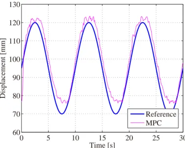
dictive control (MPC). Although the control performance of MPC is the best, the difference of them are small for under no-load condition. Under loaded condition (3.5 kg), the performance of MPC becomes worst due to accuracy of the nominal model. Note that the performance of MRAC under loaded condition can be improved because MRAC has adaptive parameter estimation algorithm. However, the characteristics of the muscle consistently change and then the adaptive algorithm con-sistently work. It means that the muscle parameters are updated under transient response at all times. This leads degradation of the control performance because MRAC cannot ensure transient response.

To solve the problem of MPC under loaded condition, recursive least squares (RLS) algorithm is applied to the control method. RLS algorithm can update the parameters of the muscle on real-time basis. In addition, its convergence is faster than the speed of MRAC. Hence, adaptive model predictive control (AMPC) can control the muscle displacement under loaded condition. Additional improvement is the use of multiple coincident points for MPC and AMPC. When prediction horizon is set to 5 steps, which means 0.5 s here, the control performance of both control methods, which use only one coincident point, is degraded because of failure of prediction. For this problem, the use of multiple coincident points and evaluation function are proposed. This can take into account of all predicted error in prediction horizon.

We also propose predictive On/Off control to improve the control performance of On/Off con-trol when only On/Off valves are used in muscle systems because the performance of the valves is lower than the performance of the servo and proportional valves, although On/Off valves are gen-erally cheaper than the servo and proportional valves. The proposed On/Off control is based on the concept of MPC, which are one-step-ahead estimation and evaluation function. The proposed control method can consider the predicted muscle displacement and then can reduce the undesirable switching of the valves. Hence, it is shown that the On/Off control can be improved by using the concept of MPC.

muscles because it can be easily possible to implement. In addition, the control performance of the displacement control with estimation method II is shown by experiment and then it is shown that the maximum steady-state error is less than 5 mm.

I wish to express my deepest gratitude to my supervisor Professor Kazuhisa Ito of Department of Machinery and control Systems, Systems Engineering and Science, Shibaura Institute of Technol-ogy, for his enthusiastic guidance, numerous useful advices, and helpful technical support.

I would like to thank Professor Pierluigi Beomonte Zobel of Department of Industrial and In-formation Engineer and Economics, University of L’Aquila, Italy, for not only technical support but also his hospitality during my stay in Italy for exchange program.

I would also like to thank Professor Shin-ichirou Yamamoto of Department of Bioscience and Engineering, Systems Engineering and Science, Shibaura Institute of Technology.

My special thanks are to all members of Environment and System Control Laboratory. Special thanks to Takashi Okamoto, Kouichi Teraoka, and Keiichiro Yasumori. Without their contribution and support, this work would not have been possible.

By virtue of the above supports, the dissertation has been successfully accomplished.

1 Introduction 1

1.1 Background and motivation . . . 1

1.2 Modeling of tap-water driven McKibben muscles . . . 3

1.3 Load compensation for McKibben muscles . . . 4

1.4 Research objectives . . . 5

2 Composition of the dissertation 7 3 Tap-water driven McKibben muscles 10 3.1 Introduction . . . 10

3.2 Working principle of McKibben muscles[17] . . . 12

3.3 Characteristics of McKibben muscles . . . 13

3.3.1 Experimental conditions . . . 14

3.3.2 Contraction force - pressure characteristics . . . 16

3.3.3 Discussion . . . 17

3.3.4 Displacement - pressure characteristics . . . 18

3.3.5 Discussion . . . 20

3.4 Applications of McKibben muscles . . . 21

3.4.1 Rehabilitation engineering . . . 22

3.4.2 Gait-training orthosis . . . 23

3.4.3 Hydrotherapy and underwater gait-training . . . 26

4 Modeling of McKibben muscle 28

4.1 Introduction . . . 28

4.2 Static muscle model . . . 30

4.2.1 Static model of McKibben muscle . . . 31

4.2.2 Modified static model . . . 33

4.3 Experimental validation of static models . . . 33

4.3.1 Discussion . . . 34

4.4 Muscle model based on linear system identification . . . 35

4.4.1 Experiments of pre-identification . . . 35

4.4.2 Experiments of identification . . . 37

4.5 Modified model with Bouc-Wen hysteretic model . . . 39

4.6 Evaluation of proposed model . . . 42

4.6.1 Hysteresis analysis . . . 42

4.6.2 Analysis of load effect . . . 44

5 Controller design 47 5.1 Introduction . . . 47 5.2 PID control . . . 48 5.2.1 Experiment of PI control . . . 49 5.2.2 Discussion . . . 51 5.3 Adaptive control . . . 52

5.3.1 Modified nominal muscle model . . . 52

5.3.2 Methodology of MRAC (projection algorithm) . . . 53

5.3.3 Experiment of MRAC: Projection algorithm . . . 54

5.3.4 Discussion: MRAC (projection algorithm) . . . 57

5.4 Model predictive control (MPC): One coincident case . . . 57

5.4.1 Methodology of MPC: One coincident case . . . 58

5.4.2 Experiment of MPC: One coincident point case . . . 59

5.4.3 Discussion . . . 63

5.5 Adaptive model predictive control (AMPC) . . . 64

5.5.1 RLS algorithm . . . 65

5.5.3 Experiment of AMPC . . . 69

5.5.4 Discussion . . . 72

5.6 MPC: Multiple coincident points case . . . 73

5.6.1 Methodology of MPC: Multiple coincident points case . . . 73

5.6.2 Modification of nominal model . . . 76

5.6.3 Experimental results of MPC: Multiple coincident points case . . . 77

5.6.4 Experimental results of AMPC: Multiple coincident points case . . . 80

5.6.5 Discussion . . . 85

5.7 Comparative analysis on muscle model . . . 87

5.8 Predictive On/Off control . . . 92

5.8.1 Methodology of predictive On/Off control . . . 93

5.8.2 Experiment of predictive On/Off control . . . 96

5.8.3 Discussion . . . 97

6 Estimation of muscle displacement 100 6.1 Introduction . . . 100

6.2 Estimation method I (flex sensor) . . . 101

6.2.1 Experiment of estimation method I . . . 102

6.2.2 Discussion: Estimation method I . . . 103

6.3 Estimation method II (flowmeter) . . . 104

6.3.1 Experiment of estimation method II . . . 105

6.3.2 Discussion: Estimation method II . . . 109

6.3.3 Displacement control (application of method II) . . . 110

6.4 Modified estimation method II (flowmeter) . . . 111

6.4.1 Experiment of modified estimation method II . . . 114

6.4.2 Discussion: Modified estimation method II . . . 115

6.4.3 Displacement control (application of modified method II) . . . 115

7 Conclusions 118

1.1 Change of population composition by age group-Japan: 1950 to 2055[1] . . . 2

1.2 McKibben artificial muscles . . . 3

1.3 Comparison of contraction rate with loads . . . 4

2.1 Flow chart of the dissertation . . . 9

3.1 Inner tube and braided sleeve of McKibben muscle . . . 10

3.2 Braided sleeve of the muscles [17] . . . 13

3.3 Experimental setup . . . 14

3.4 Contraction force (length: 540 mm) . . . 16

3.5 Contraction force (length: 513 mm) . . . 16

3.6 Contraction force (length: 486 mm) . . . 17

3.7 Contraction force (length: 459 mm) . . . 17

3.8 Contraction force (length: 432 mm) . . . 17

3.9 Contraction force (length: 405 mm) . . . 17

3.10 Experimental results of contraction force - pressure characteristics . . . 18

3.11 Experimental result (0.27 MPa) . . . 19

3.12 Experimental result (0.2 MPa) . . . 19

3.13 Displacement - pressure characteristics . . . 20

3.14 Rehabilitation devices using McKibben muscles[19] . . . 21

3.15 Rehabilitation devices using McKibben muscles[22] . . . 21

3.16 Robotics using McKibben muscles[26] . . . 22

3.17 Robotics using McKibben muscles[27] . . . 22

3.18 Body weight support treadmill training[33] . . . 25

3.19 Underwater gait-training orthosis[45] . . . 26

4.1 Geometry of McKibben muscle . . . 31

4.2 Experimental results of contraction rate with 5 kg load . . . 34

4.3 Experimental results of contraction rate with 10 kg load . . . 34

4.4 Experiment of step response (pre-identification) . . . 36

4.5 Reliable identified bandwidth . . . 36

4.6 Input and output singnal for identification . . . 37

4.7 Comparison of identified and measured data . . . 38

4.8 Hysteresis loop of McKibben muscles . . . 39

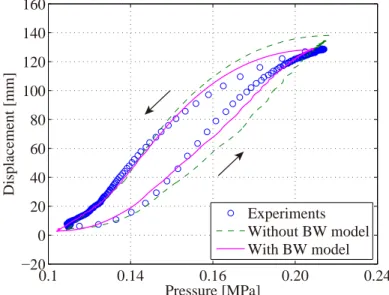
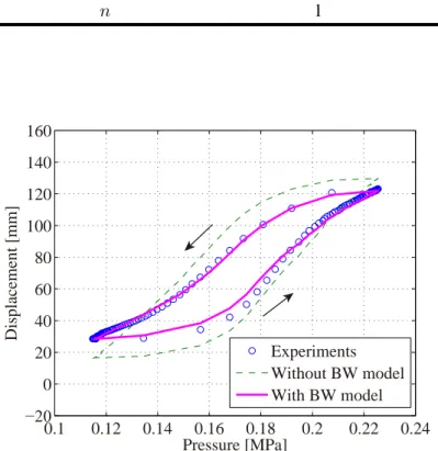
4.9 Comparison of hysteresis loop . . . 43

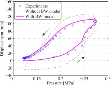
4.10 Comparison of hysteresis loop with load: 3.5kgf . . . 44

4.11 Hysteresis loop of re-identified model with load: 3.5kg . . . 45

4.12 Hysteresis loop of re-identified model with load: 7.0kgf . . . 46

5.1 Block diagram of PI control . . . 48

5.2 Experimental result of PI control (sampling period: 0.01 s) . . . 49

5.3 Experimental result of PI control (sampling period: 0.1 s) . . . 50

5.4 Experimental result of PI control with a load: 3.5 kgf (Kp= 0.65, Ki= 12.12) . . 50

5.5 Experimental result of PI control with a load: 3.5 kgf (Kp= 1.363, Ki = 0.431) . 51 5.6 Comparison of measured and identified data Eq. (5.1) (input: applied voltage for valves, output: muscle displacement) . . . 53

5.7 Experimental result of MRAC . . . 55

5.8 Parameter estimation of MRAC . . . 55

5.9 Experimental result of MRAC (load: 3.5 kgf) . . . 56

5.10 Parameter estimation of MRAC (load: 3.5 kgf) . . . 56

5.11 Concept of MPC (one coincident case) . . . 59

5.12 Experimental result of MPC . . . 60

5.13 Applied voltage for valve (MPC) . . . 61

5.15 Applied voltage for valve (Load: 3.5 kgf) . . . 62

5.16 Experimental result of MPC with load: 3.5 kgf . . . 62

5.17 Applied voltage for valve (Load: 3.5 kgf) . . . 63

5.18 Block diagram of MPC with RLS algorithm . . . 65

5.19 Rectangular window . . . 68

5.20 Experimental result of AMPC . . . 70

5.21 Parameter estimation by RLS algorithm . . . 70

5.22 Experimental result of AMPC . . . 71

5.23 One-step-ahead estimation at the first 30 seconds . . . 71

5.24 One-step-ahead estimation at the last 30 seconds . . . 72

5.25 Experimental result of MPC using one coincident point: 0.1 Hz (Hp= 5) . . . 78

5.26 Experimental result of MPC using one coincident point: 0.2 Hz (Hp= 5) . . . 78

5.27 Experimental result of MPC using four coincident points: 0.1 Hz (Hp= 4) . . . . 79

5.28 Experimental result of MPC using four coincident points: 0.2 Hz (Hp= 4) . . . . 79

5.29 Experimental result of MPC using five coincident points: 0.1 Hz (Hp = 5) . . . 80

5.30 Experimental result of MPC using five coincident points: 0.2 Hz (Hp = 5) . . . 80

5.31 Experimental result of AMPC: load 3.5 kgf (0.1 Hz, Hp = 5) . . . 81

5.32 Parameter estimation of AMPC: load 3.5 kgf (0.1 Hz, Hp= 5) . . . 82

5.33 One-step-ahead estimation of AMPC: load 3.5 kgf (0.1 Hz, Hp = 5) . . . 82

5.34 Experimental result of AMPC using five coincident points: load 3.5 kgf (0.2 Hz, Hp= 5) . . . 83

5.35 Parameter estimation of AMPC: load 3.5 kgf (0.2 Hz, Hp= 5) . . . 83

5.36 One-step-ahead estimation of AMPC: load 3.5 kgf (0.2 Hz, Hp = 5) . . . 84

5.37 Experimental result of AMPC: load 3.5 kgf (0.3 Hz, Hp= 5) . . . 84

5.38 Experimental result of AMPC: load 3.5 kgf (0.5 Hz, Hp= 5) . . . 84

5.40 Parameter estimation of AMPC:

load 3.5 kgf (0.5 Hz, Hp= 5) . . . 85

5.41 One-step-ahead estimation of AMPC: load 3.5 kgf (0.3 Hz, Hp= 5) . . . 85

5.42 One-step-ahead estimation of AMPC: load 3.5 kgf (0.5 Hz, Hp= 5) . . . 85

5.43 Magnified view of experimental result (Fig. 5.25) . . . 86

5.44 Comparison of one-step-ahead estimation . . . 88

5.45 Time response of displacement control (MPC) . . . 88

5.46 Comparison of one-step-ahead estimation (α = 0.935) . . . . 89

5.47 Time response of displacement control (α = 0.935) . . . . 89

5.48 Comparison of one-step-ahead estimation (α = 0) . . . . 90

5.49 Time response of displacement control (α = 0) . . . . 90

5.50 Simulation results of 0.001 Hz as a reference frequency . . . 91

5.51 Simulation results of 0.5 Hz as a reference frequency . . . 91

5.52 Flow chart of the predictive On/Off control . . . 93

5.53 Comparison result of the simulated displacement of the one-step-ahead estimation with the measured displacement . . . 94

5.54 Experimental result of predictive On/Off control . . . 96

5.55 Magnified view of input signal of predictive On/Off control (15 to 20 s) . . . 96

5.56 Magnified view of Fig. 5.54(10 to 20 s) . . . 97

5.57 Comparison of Eq. (5.55) and (5.56) . . . 99

6.1 Flex sensor (length: 2.2inch, spectrasymbol) . . . 101

6.2 Calibration of flex sensor . . . 102

6.3 Estimation results with flex sensor: 500 mm in natural length . . . 103

6.4 Estimation results with flex sensor: 400 mm in natural length . . . 103

6.5 Experimental setup for estimation method II . . . 105

6.6 Experimental result of flow rate and displacement (no load) . . . 107

6.8 Measured and estimated muscle displacement by Method II (load: 3.5 kgf): dot-line indicates the measured displacement without time delay, solid-dot-line indicates

the measured displacement with time delay (0.5 s) . . . 108

6.9 Measured and estimated muscle displacement by Method II (no load) . . . 108

6.10 Comparison of supply pressure: dot-line indicates under loaded condition and solid-line indicates under no load condition . . . 109

6.11 Experimental result of displacement control with estimation method II . . . 110

6.12 Modified experimental setup using two flowmeters . . . 111

6.13 Muscle displacement and inlet and outlet flow measured by FM1 and FM2 . . . 112

6.14 Displacement - volume characteristics . . . 113

6.15 Experimental result of estimation (rectangular signal) . . . 114

6.16 Experimental result of estimation under loaded condition (sinusoidal signal) . . . . 114

6.17 Displacement control with estimation under no-load condition . . . 116

6.18 Displacement control with estimation under loaded condition . . . 116

3.1 Proportional valve: PV (KFPV300, Koganei Corporation) . . . 15

3.2 Pressure sensor (PVL10KD,KYOWA ELECTRONIC INSTRUMENTS CO., LTD.) . . 15

3.3 Load cell (LUX-B-2KN-ID,KYOWA ELECTRONIC INSTRUMENTS CO., LTD.) . . 15

3.4 Potentiometer (SR1A-62, Celesco Transducer Products, Inc.) . . . 15

3.5 Calibration of load cell . . . 16

4.1 Classification of Bouc-Wen model . . . 41

4.2 Identified hysteresis parameters of proposed model Eq. (4.25) . . . 42

4.3 Identified hysteresis parameters of proposed model: load 3.5 kgf . . . 45

5.1 Experimental conditions for MPC[71] . . . 60

5.2 Comparison analysis of experimental results (PI vs. MPC) . . . 63

5.3 Identified hysteresis parameters of proposed model Eq. (5.58) . . . 95

5.4 Comparison analysis of experimental results . . . 97

5.5 Input signal of the proposed controller . . . 98

6.1 Flowmeter (FD-M10AY, KEYENCE CORPORSTION) . . . 106

6.2 Measured parameters of the muscle . . . 106

6.3 Flowmeter: FM1(NDV10-STD1, Aichi Tokei Denki Co., LTD.) . . . 112

6.4 Flowmeter: FM2(OF10ZAT, Aichi Tokei Denki Co., LTD.) . . . 112

A, n, α, β, γ : Hysteresis parameters [·]

D(k) : Outer diameter of muscle [m]

F (k) : Normal function [·]

Gi(z) : Transfer function of muscle (i = 1, 2, 3, 4) [·]

Hp : Prediction horizon [step]

J (k) : Evaluation function [·]

L(k) : Muscle length [m]

L0 : Natural length of muscle [m]

P (k) : Covariance matrix [·]

Q(k) : Weight matrix of error [·]

R(k) : Weight matrix of input [·]

S(Hp) : Step response [·]

Ts : Sampling period [s]

U (z) : Applied voltage [V]

V (k) : Volume of muscle [m3]

a(k) : Gain constant [·]

b : Thread length [m]

e(k) : Error [m]

ki : Integral gain [V/m]

kp : Proportional gain [V/m]

l(k) : Muscle displacement [m]

p(k) : Supply pressure [MPa]

q(k) : sum of flow [L]

r0 : Diameter of inner tube [m]

u(k) : Input [V]

x(t) : Displacement [m]

w(k) : Hysteresis state variable [·]

y(k) : Output [m]

γm : Angle between axis and a thread [rad]

η : Contraction rate [·]

θ(k) : Parameter vector [·]

ˆ

θ(k) : Estimated parameter vector [·]

ϕ(k) : Regression vector [·]

Subscript

0 : Initial condition

Acronyms

ADL Activities of daily living

AMPC Adaptive model predictive control ARX Auto-regressive ex-ogenous BIBO bounded input - bounded output BWSTT Body weight support treadmill training KAFO Knee-ankle-foot orthosis

MPC Model predictive control

MRAC Model reference adaptive control QOL Quality of life

Introduction

1.1

Background and motivation

Engineering technology for medical and welfare fields has been strongly required year by year because elderly society is one of the critical issues all over the world. In particular, it is a serious problem in Japan as seen in Fig. 1.1[1]. Its population under 15 years old is 16,803 thousand (13.2% of the total population), the population from 15 to 64 years old is 81,032 thousand (63.8%), and the population over 65 years old is 29,246 thousand (23.0%) in 2010. The population under 15 years old have decreased by 718 thousand from 2005 but its over 65 years old increased by 3,574 thousand.

Decrease of younger people means decrease of workers in these fields, on the other hand, in-crease of elderly people means inin-crease of people who need medical helps. Thus, substitution of human resources by engineering technology is essential for the situation.

Development of rehabilitation systems demands various knowledge of rehabilitation. In other words, medical and welfare systems without consideration of users or patients have no sense. It has often been a wall between engineers and users. Rehabilitation engineering is not only diversion of industrial mechanical engineering. Important priorities requiring for rehabilitation engineering are safeness and human friendliness, although performance and efficiency are also important factors. Thus, rehabilitation systems must be developed with special attention to humans.

0 2,000 4,000 6,000 8,000 10,000 12,000 14,000 2055 2050 2040 2030 2020 2010 2005 2000 1990 1980 1970 1960 1950 Population (10 thousand persons) Actual Figures (Population Census) Estimates of FY2012 (Population Projection for Japan)

Population 14 or younger Population aged 15-64 Population 65 or older Percentage of productive-age population (aged 15-64) Elderly rate

(percentage of population 65 or older)

Total fertility rate

Total fertility rate 1.35 Elderly rate 39.4% Percentage of productive-age population 51.2% 65.8 (2005) 20.1 (2005) Population peak (2004) 12,779 1.26 (2005) 2,567 3,685 6,773 1,203 ₈₆₁ 4,706 3,626 9,193 11,661 8,409 12,728 1,752

Sources: Up to 2010 - “Population Census”, Statistics Bureau, Ministry of Internal Affairs and Communications From 2015 on - “Population Projection for Japan (estimated in January 2012)”,

National Institute of Population and Social Security Research

Fig. 1.1: Change of population composition by age group-Japan: 1950 to 2055[1]

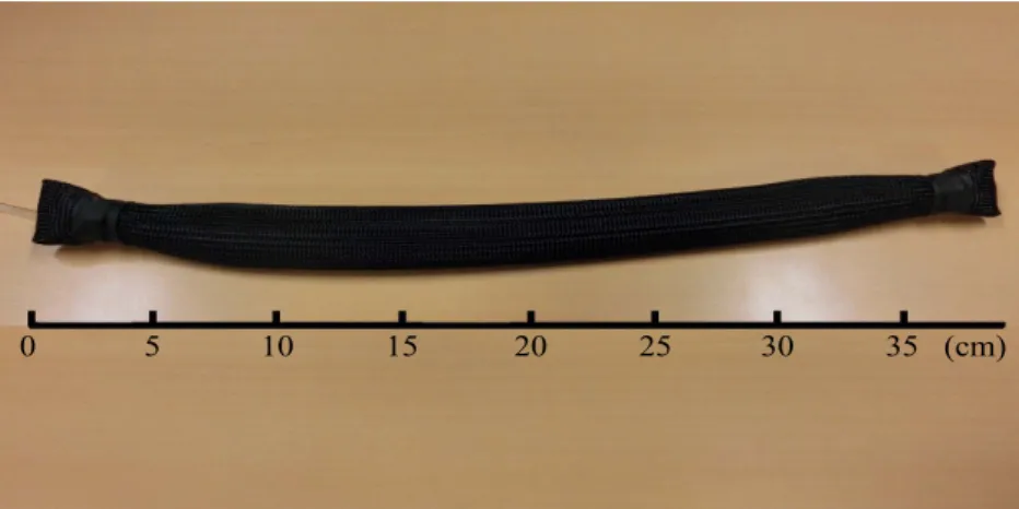
This study is concerned with McKibben muscles as actuators for such systems. Figure 1.2 shows a photo of a McKibben muscle. McKibben muscles, in general, consist of inner rubber tube and outer nylon sleeve[2]. The muscles have some advantages as actuators of rehabilitation systems: 1) Light weight, 2) High power-to-weight ratio, 3) High flexibility, and 4) Low cost[3]. In particular, 1) and 3) are suitable for rehabilitation. Inherent redundancy attributed their structures is also preferable.

On the other hand, there are two problems: The one is driving source and the other is the control performance. In fact, the muscles require compressors as driving sources in pneumatics. Notice that there are only narrow spaces for rehabilitation devices in hospitals. In addition, compressors make noise and vibration, which give discomfortable feelings to patients.

muscles due to components such as rubber tube and nylon sleeve should be a problem.

From these backgrounds, we focus on water hydraulic McKibben muscles, especially tap-water driven McKibben muscles. The muscles use tap-water as a driving source because it is no need to use certain power source devices such as compressors or hydraulic pumps.

Application of tap-water can solve the problem mentioned above, that is, installation spaces in hospitals. This also has additional effects on rehabilitation. It is suitable for patients to use water hydraulics, which have 100% oil-free characteristics[5], especially for underwater rehabilitation. Moreover, faster response than the one of pneumatic McKibben muscles is expected when water is used as working fluid because water is incompressible fluid. Thus, tap-water driven McKibben muscles have lots of advantages for rehabilitation.

Fig. 1.2: McKibben artificial muscles

1.2

Modeling of tap-water driven McKibben muscles

on accuracy of nominal models, which can express behavior of plants.

On the other hand, modeling of McKibben muscles is difficult because the muscles have strong nonlinearities. In pneumatic McKibben muscles, compressibility has also to be taken into consider-ation. If complexity of models is allowed, we can derive precise models but control laws generally require simple models. The important point here is how to get simple models of the muscles. Un-fortunately, there is no such an appropriate model with simple structure and high accuracy.

1.3

Load compensation for McKibben muscles

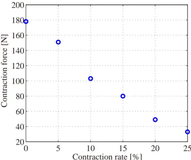
Load compensation is another considerable point in control[10], especially the applied controls are model-based controls because loads can easily degrade the control performance. Figure 1.3 shows the experimental results with three types of loads: 50N, 100N, and 150N.

0

0.05

0.1

0.15

0.2

0.25

0.3

0.35

0

0.1

0.2

0.3

0.4

Pressure [MPa]

Contraction rate [

•]

Fig. 1.3: Comparison of contraction rate with loads

muscles.

1.4

Research objectives

This study is concerned with tap-water driven McKibben muscles as actuators of rehabilitation systems. “Tap-water driven” here means systems driven by tap-water pressure. The main purposes of this study are modeling of the muscles for the model-based controller and design of model-based controllers. Then they includes methods to figure out the characteristics, that is contraction rate -supply pressure characteristics, of tap-water driven McKibben muscles. Note that there is additional purpose of this study: It is an application of the muscles to gait-training orthoses. Some of research objectives are concerned with the orthoses.

The detail of research objectives are as follows.

1. Derivation of precise and simple models of the muscles

Linear system identification method, which is based on only relationship between inputs (sup-ply pressure or applied voltage for control valves) and outputs (displacement of the muscles), is applied to derivation of the muscle models. This method is expected to simplify muscle models because water as working fluid is incompressible and temperature dynamics can be neglected. In pneumatic McKibben muscles, it is required to take account of compressibility and also temperature dynamics. This is, however, only linear theory and it is obvious that nonlinearities of the muscles such as hysteresis are neglected.

2. Application of Bouc-Wen hysteresis model

To compensate the nonlinearities neglected in the derived simple linear model of the muscles, we propose combination of a hysteresis model, which is widely used in various fields. As the simple model can be obtained by system identification method, the hysteresis model can easily be applied. The modified model can be used for not only a nominal model of model-based control but also static analyses such as hysteresis analysis.

3. Controller design

com-pared with conventional PID controller. In particular, experiment with some loads show considerable problem of the muscle.

4. Adaptive parameter estimation

Load compensation by adaptive parameter estimation is proposed, specifically recursive least squares (RLS) algorithm is applied to the system. In addition, modeling error can be compen-sated by the algorithm in real-time basis. The effectiveness of the proposed method is shown by some experiment with/without loads.

5. Displacement estimation method

Composition of the dissertation

In Chap. 3, contraction force - supply pressure and contraction rate - supply pressure charac-teristics of tap-water driven McKibben muscles are shown and some applications of conventional McKibben muscles are introduced. In particular, the applications, for which the tap-water driven muscles should be used, are suggested. In addition, conventional rehabilitation systems are intro-duced and then some advantages and disadvantages of them are also presented.

In Chap. 4, models of the muscles are proposed and validity of the models is confirmed by analyses of contraction rate - supply pressure and hysteresis characteristics. The proposed model consists of a simple model derived by system identification method and Bouc-Wen hysteresis model. Then discussion about loads is made because they significantly effect on the response of the mus-cles. Note that there is few consideration about loads, although muscle models including Bouc-Wen hysteresis model have been already proposed.

In Chap. 5, two experimental setups are constructed: The one consists of proportional valves and another consists of only On/Off valves. For the setup with proportional valves, three control laws are applied to the muscles. The one is PID control, which is a conventional control for the muscle displacement control. The others are model reference adaptive control (MRAC) and model predictive control (MPC), which are model-based control methods. The control performances of these controllers are examined by experiment. In particular, MPC assumes that nominal models are completely identified plants but the models surely have modeling errors in practice. This leads inevitable degradation of the control performance of MPC. An adaptive parameter estimation

gorithm, which is recursive least squares method, is combined to overcome the error caused by modeling. Moreover, the number of coincident points is considered in MPC at design steps and the results are compared with the results of PID, MRAC, and conventional MPC.

On the other hand, for the setup with On/Off valves, conventional On/Off control and predictive On/Off control, which is based on a concept of MPC, are applied and compared.

Chapter 3: Tap-water driven McKibben muscles

Chapter 4: Modeling of McKibben muscles

Chapter 5: Controller design

Principle and characteristics of the muscles

Applications of the muscles (Related work)

Chapter 6: Estimation of muscle displacement

Muscle model derived by system identification Static muscle models

Modified muscle model with Bouc-Wen model

Hysteresis analysis of proposed model Validation of static models

Model-based controls (MRACS, MPC) Conventional PI control

Comparative analysis for control performance of applied controls (PI, MRACS, MPC)

Adaptive model predictive control with RLS

Validation of load compensation

Comparative analysis for proposed estimation methods

Measurement method I with flex sensor Measurement method II with flowmeter

Displacement control with estimated displacement (PI with measurement method II)

Fig. 2.1: Flow chart of the dissertation

Tap-water driven McKibben muscles

3.1

Introduction

McKibben muscles are one of the feasible actuators for medical and welfare systems. Advantages of the muscles are following: 1) Light weight, 2) High power-to-weight ratio, 3) High flexibility, and 4) Low cost. These are suitable for such systems because human friendliness is the most important factor and highly required. Generally, electric motors, pneumatic compressors, or hydraulic pumps are used as driving sources but they are unsuitable in that sense. The muscles were invented in the 1950s by Joseph L. McKibben[11], [12] to motorize arm orthoses and help handicapped hands. They consist of an inner rubber tube and outer braided sleeve (Fig. 3.1) and are closed by two joints. They are usually driven by pneumatics, and when the inner tube is pressurized, gas inside the tube pushes inner surface of the tube and then increases its volume. The muscles can shorten due to non-extensibility of the sleeve. This is almost same motion as human skeletal muscles.

Sleeve

Rubber tube

Joint

Fig. 3.1: Inner tube and braided sleeve of McKibben muscle

Relationship between supply pressure, muscle displacement, and contraction force are major characteristics of the muscles. Human skeletal muscles also have particular characteristics: 1) Convex shape active tension - length relationship, 2) Nonlinear passive tension - length relationship, and 3) Hyperbolic tension - velocity relationship[13]. Although the characteristics of the McKibben muscles are completely same characteristics as human skeletal muscles, this should be emphasized because most of actuators cannot have the characteristics and be important for medical and welfare systems.

A conventional driving source of these kind of muscles is pneumatics. As that is well known, pneumatics is an easy-to-use driving source because pressure medium is air. Pressure range of pneumatics covers rated pressure range of the muscles. If compressed air leaks from the muscles or pneumatic circuits, they slightly damage environment and also humans. In addition, compressibility of air helps system softness. On the other hand, compressibility of air degrades system response. Pneumatics requires compressors and their installation spaces. In general, compressors make noise and vibration and then these aspects critically come to problems.

A solution of these problems is water hydraulics, especially tap-water here. Water hydraulics has faster response than the one of pneumatics due to characteristics of water as working fluid. Moreover, water hydraulics has a unique characteristics, which is 100% oil-free. This means that water hydraulics has higher human friendliness than pneumatics. More importantly, tap-water driven McKibben muscles need no driving source devices such as compressors or hydraulic pumps when tap water, whose pressure level is approximately less than 0.3 MPa, can generally be avail-able. Although the pressure level of tap-water is less than the level of pneumatics, the omission of driving source devices is attractive for medical and welfare fields. In other words, the tap-water driven McKibben muscles are available for anywhere with a tap. This leads to wider applications of them. Thus, it is useful to create synergy effects between advantages of the McKibben muscles and advantages of water hydraulics.

Notice that there are also disadvantages of the tap-water driven muscles. Water as a working fluid is heavier than air as pressure medium. This means the muscles are also heavier when water is supplied to the muscles. Thereby, when the muscles are attached to rehabilitation systems or power-assist suits, the weights may be troubles.

pneu-matics whenever compressed air is leaked. In water hydraulics, however, leaked water swamps the systems and also environment. Moreover, McKibben muscles in general are breakable because the main material of the muscles is synthetic rubber and the rubber may burst during operation.

There are other types of water hydraulic McKibben muscles[14], [15]. In particular, the muscles can be used in higher pressure range, which is more than 1 MPa, because pneumatics is less than 1 MPa basically and there is no way to apply such a high pressure range. These types of muscles have been applied to industrial machineries and robotics[16]. The structures, materials, and production methods of the muscles have been improved in order to withstand the high pressure and enhance life cycle of the muscles. In contrast with that types of the muscles, water hydraulic muscles driven by tap-water have same structure, materials, and production methods of the pneumatic muscles because the pressure range of a tap is almost same level as the pneumatic muscles. Thus, the water hydraulic muscles can be classified by pressure range or driving sources (hydraulic pumps or tap-water).

For the purposes of modeling and control, it is required to simplify muscle models. There are many models describing the muscle characteristics but each model has trade-off between accuracy and simplicity, especially the pneumatic muscles have some considerable characteristics such as compressibility and temperature dynamics. On the other hand, the water hydraulic muscles have no such characteristics and should be simplified. The details are discussed in Chap. 4.

3.2

Working principle of McKibben muscles[17]

Braided Thread Elementary Pantograph ψ r0 L0

Braided Sleeve Thin-Wall Rubber_{Inner Tube}

ψ

Fig. 3.2: Braided sleeve of the muscles [17]

Parameters characterizing the shapes of the muscles are initial braid angle γm and initial muscle

length L0. The initial braid angle γm and the initial muscle length L0 are defined as the angle

between the muscle axis and the braided thread before expansion and the initial length of the sleeve of the muscles, respectively. The other is initial muscle radius noted r0, which is defined as the

radius of the inner rubber tube. Note that this definition involves a consideration of a thin inner tube and then the radius r0 indicates the initial internal radius of the muscle sleeve.

In these geometrical parameters of the muscles, the following are neglected: 1) Conic shapes at the ends of the muscle, and 2) Intrinsic mechanical aspects of the braided threads and inner tube. To take into consideration of conic shapes is particularly complex for modeling of the muscles. For second point in detail, the braided thread is assumed to be unstretchable and without any distortions.

3.3

Characteristics of McKibben muscles

3.3.1 Experimental conditions

Figure 3.3 shows an experimental setup for tap-water driven McKibben muscles. The setup consists of the muscle, two proportional valves, pressure sensor, load cell, linear potentiometer, and PC. The details of them are listed in Tables 3.1 to 3.4. Note that a pair of the proportional valves used in this setup, which are two-port two-position valves, is applied to construct a three-port three-position proportional valve in Fig. 3.3 in order to simplify the symbol because no commercialized three-port three-position proportional valves are available and we use the combination of the valves with same function as a three-port three-position valves. Plastic tubes are used for the experimental circuit to connect components. Maximum pressure of tap-water as a driving source is approximately 0.25 to 0.3 MPa but it is depends on situations. Applied voltage source for each instruments is PC with MATLAB and dSPACE, which is a real-time control system including AD/DA converters.

AD DA PC PV f (k) u(k) p(k) Load cell

Table 3.1: Proportional valve: PV (KFPV300, Koganei Corporation) Working fluid Air, neutral gas, and water Structure 2 ports and 2 positions Operation type Direct action type Circuit configuration Normally closed Operation pressure range 0.1 to 0.3 MPa

Cv value 1.60

Range of temperature -10 to 90◦C (no freezing allowed)

Water proof IP65 equivalent

Table 3.2: Pressure sensor (PVL10KD,KYOWA ELECTRONIC INSTRUMENTS CO., LTD.)

Rated pressure 1 MPa

Output signal 0 to 5 V

Material of body SUS

Range of temperature -10 to 60◦C

Applied voltage 12 V DC

Water proof IP61

Table 3.3: Load cell (LUX-B-2KN-ID,KYOWA ELECTRONIC INSTRUMENTS CO., LTD.)

Rated force ± 20 kN

Input resistance 375 Ω± 1.5%

Rated output ± 1.3 mV/V

Range of Temperature -20 to 80 ◦C Range of applied voltage 1 to 10 V AC or DC

Water proof IP67

Table 3.4: Potentiometer (SR1A-62, Celesco Transducer Products, Inc.) Range of measurement 0 to 1575 mm

Rated applied voltage 30 V Range of Temperature -40 to 85◦C

Rated velocity 2000 mm/s

Tensional force of wire 6.4 N± 30%

3.3.2 Contraction force - pressure characteristics

This section shows the relationship between supply pressure and contraction force of the muscles. In these isometric experiments, the muscle is 540 mm in natural length, and the supply pressure by tap-water is approximately 0.27 MPa. The load cell fixed bottom of the setup is connected with the muscle in series. Calibration of the load cell is shown in Table 3.5 by Eq. (3.1).

Fl= yo× h (3.1)

where Flis an external force, yooutput of load cell (mV/V), and h calibration coefficient: 0.0006496

kN/1.0×10−6, which is given by manufacturer.

Table 3.5: Calibration of load cell

Weight [kg] 1.01 2.50 4.97 7.47 9.95 14.97 Indicated force [N] 10.6 25.5 48.4 75.5 99.5 148.4

Figures 3.4 - 3.9 show the transient response of the supply pressures and the contraction force of the muscle in 5% increments from natural length of the muscle. Input signal 10 V (rated voltage) for the valve are applied at 10 s and the load cell connected with the bottom of the muscle measures the contraction force. Note that contraction rate of the muscle is adjusted by changing positions of the top end of the muscle fixed on the setup.

0 5 10 15 20 0 50 100 150 200 Time [s] Force [N] 5 10 15 200 0.1 0.2 0.3 0.4 Pressure [MPa] Contraction force Pressure

Fig. 3.4: Contraction force (length: 540 mm)

5 10 15 20 0 50 100 150 200 Time [s] Force [N] 0 5 10 15 200 0.1 0.2 0.3 0.4 Time [s] Pressure [MPa] Contraction force Pressure

0 5 10 15 20 0 50 100 150 200 Time [s] Force [N] 5 10 15 200 0.1 0.2 0.3 0.4 Time [s] Pressure [MPa] Pressure Contraction force

Fig. 3.6: Contraction force (length: 486 mm)

0 5 10 15 20 0 50 100 150 200 Time [s] Force [N] 5 10 15 200 0.1 0.2 0.3 0.4 Time [s] Pressure [MPa] Contraction force Pressure

Fig. 3.7: Contraction force (length: 459 mm)

0 5 10 15 20 0 50 100 150 200 Time [s] Force [N] 5 10 15 200 0.1 0.2 0.3 0.4 Pressure [MPa] Pressure Contraction force

Fig. 3.8: Contraction force (length: 432 mm)

0 5 10 15 20 0 50 100 150 200 Time [s] Force [N] 5 10 15 200 0.1 0.2 0.3 0.4 Time [s] Pressure [MPa] Pressure Contraction force

Fig. 3.9: Contraction force (length: 405 mm)

3.3.3 Discussion

It is obvious that the pressure inside the muscle can reach the maximum pressure 0.25 MPa for all experiments. Then contraction forces of each experiments depend on the initial condition of muscle length. Contraction force in natural length is the largest and it decreases in proportion to contraction rate. Braid angle of the muscle is attributed to the difference of maximum contraction forces. The larger the contraction rate is, the thinner pantograph shaped by braided threads is. Thereby, vertical force acting the pantograph is smaller than horizontal force acting the pantograph.

contraction rate because contraction times, which indicate the time to contract 5% to 25%, increase in proportion to contraction rate. However, steady-state values of contraction force are constant and then we can compare these results and characterize the contraction force - pressure relation as shown in Fig. 3.10. These results and related experimental results [18] for pneumatic muscles have same tendency for this aspect. Thus water hydraulic McKibben muscles have same contraction force level as pneumatic one. Note that maximum pressure of tap-water is less than conventional maximum pressure of pneumatics. In addition, dynamics comparison between water hydraulic and pneumatic muscles is difficult from these results because the transient response depends on experimental circuits and components.

0 5 10 15 20 25 20 40 60 80 100 120 140 160 180 200 Contraction rate [%] Contraction force [N]

Fig. 3.10: Experimental results of contraction force - pressure characteristics

3.3.4 Displacement - pressure characteristics

0 5 10 15 0 25 50 75 100 125 150 Time [s] Displacement [mm] 0 5 10 150.1 0.15 0.2 0.25 0.3 0.35 0.4 Time [s] Pressure [MPa] Displacement Supply pressure

Fig. 3.11: Experimental result (0.27 MPa)

0 5 10 15 0 25 50 75 100 125 150 Time [s] Displacement [mm] 0 5 10 150.1 0.15 0.2 0.25 0.3 0.35 0.4 Time [s] Pressure [MPa] Displacement Supply pressure

Fig. 3.12: Experimental result (0.2 MPa)

0 0.05 0.1 0.15 0.2 0.25 0.3 0.35 350

400 450 500

Supply pressure [MPa]

Muscle Length [mm]

Fig. 3.13: Displacement - pressure characteristics

3.3.5 Discussion

Displacement of McKibben muscles may be changed by natural length of the muscles and in gen-eral contraction rate, which indicates ratio of displacement to natural length of the muscles, is introduced. The contraction rate η is defined as

η = L0− L

L0

(3.2)

where L is length of the muscle, and L0natural length of the muscle.

In these experiments, proportional valves are controlled to set supply pressure as 0 to 0.26 MPa in 0.02 MPa increments. When supply pressure is 0.26 MPa, which is almost maximum pressure, the contraction rate ηmaxis obtained by

ηmax=

L0− Lmax

L0

= 0.25 (3.3)

has the same statics as pneumatic muscles. Thus water hydraulic McKibben muscles have same characteristics as pneumatic McKibben muscles.

3.4

Applications of McKibben muscles

Pneumatic McKibben muscles have already been applied to various systems such as rehabilitation devices[19]-[23], body-support suits[24], [25], and robotics[26], [27], as illustrated in Figs. 3.14 to 3.17. These developments show the applicability of the muscles. Suitably the muscles have been used for the satisfaction of human friendliness.

Fig. 3.14: Rehabilitation devices using McKibben muscles[19]

Fig. 3.16: Robotics using McKibben muscles[26]

Fig. 3.17: Robotics using McKibben muscles[27]

3.4.1 Rehabilitation engineering

using auxiliary component, for instance, artificial limbs, prosthetic orthoses, and wheelchairs[28]. Thereby, it aims to achieve domestic and social independence of patients. Rehabilitation engineer-ing contributes on multiple roles: 1) Development of auxiliary and trainengineer-ing equipment, 2) Quanti-tative analyses of training and clinical test data, 3) Systemization of rehabilitation programs, and 4) Maintenance of network systems and rehabilitation institutions. In particular, training equipment can reduce strain of PTs making patients rehabilitate themselves. In addition, high-intensity and long-term repetitive action pattern exercises can be possible by using training equipment. Then benefits from applications of training equipment are to be able to quantitatively adjust loads de-pending on knowledge of PTs and to store and analyze training data to evaluate effectiveness of rehabilitation methods and assessment of repeatability.

In particular, this study is also concerned with gait-training, which is rehabilitation for motor function, as an application of tap-water driven McKibben muscles. Reduction of motor function caused by accidents or diseases and loss of motor function with aging leads to cause loss of activities of daily living (ADL)[29] and quality of life (QOL)[30]. ADL, which introduces a new perspective on the medical community, is a key concept for adaptation from daily life. In the 1980s, the key concept of rehabilitation was changed once from ADL to QOL. Although QOL is mainstream now, ADL has not lost its importance. In fact, from “Improvement the level of ADL for QOL”, ADL has not only its importance but also connection with QOL. The recovery of gait disorder is particularly useful in ADL and QOL because gait movement, which is well known as means of migration, is one of the important elements of daily living.

3.4.2 Gait-training orthosis

Underwater gait-training is one of gait-training in rehabilitation. This is a suitable application of the muscles because water hydraulics, which has 100% oil free is desirable in the gait-training, not oil hydraulics and pneumatics. In addition, as buoyant force reduces patient’s weight under water, smaller and lighter system without any body weight support devices can be realized. This has great impact to the conventional rehabilitation systems.

cen-tral nervous systems, have never been recovered and repaired again if nerve cells were damaged once. Although some cases depend on regions of damaged spinal cords, reduction of locomotion is caused by functional loss of spinal cords. In conventional rehabilitation, an assumption that lost functions never recovered were accepted, and its purpose was to obtain compensation by using residual function. In other words, rehabilitation based on conventional methods means exercises for residual function to compensate lost function. However, an opinion for this tradition is changing tremendously because animal experiment proves plastic adaptation of central nerve and possibility of recovery by reconstruction of neural networks. A lot of researcher actively are now carrying out studies on neurorehabilitation[32].

In general, there are some gait-training with parallel bars, walkers, and sticks for PTs to make a choice on training methods according to levels of patient’s torpor and movement function. On the other hand, a new gait-training called body weight support treadmill training (BWSTT) gains much attention as seen in Fig. 3.18. In 1980s, Barbeau[12] reports on recovery of muscle activities and joint motion patterns of cats damaged spinal cord by making the cat exercise on a treadmill. BWSTT builds on a concept and apply results to practical situation. Wernig[33] reports that BWSTT is effec-tive against a large number of cases. Then availability of BWSTT against complete/incompetence spinal injury is shown and it is indicated that BWSTT has effects on recovery of walk function[34]-[37]. About BWSTT, however, harness suspending patients to compensate their body weight is needed and couple of PTs are required to move patient’s legs, and thereby these give excessive burdens for the PTs. For this reason, it is difficult to carry out effective training with BWSTT for a long time. Nevertheless, there are poorly-reproducible results because effects of training depend on experiences and subjective opinion of PT who make choices of training methods. Colombo[38] developed a training system that can support gait-training automatically and Dietz[39] reports on the effect and precautions of using the system. As seen from the above, studies on neurorehabilitation are actively made around the West. In Japan, however, these new approaches are not at bedside stage because of the restriction of Pharmaceutical Affairs Act and its cost.

by encouraging reorganization of neural network. Kojima[41] carried out experimental tests with WBC and reports paralyzed muscle activities are induced same as BWSTT by exciting lower-limb. Kakou[42] developed a walking support robot and used it in clinical practice. This consists of gait-training device, low limb function recovery system, and upper limb training support system. In particular, low-limb function recovery system is to help biped walk movement for patients who have gait disorder caused by stroke. In fact, in clinical practice, both subacute and chronic paralyzed persons have improved their gait speed and low-limb muscle strength by training with this system twenty minutes at once in five days a week and during three weeks. In addition, physical strain of PTs and enough securement of training and safe management are also referred in these studies. On the other hand, this training had little effect on activities of daily living and the severity of paralysis and spasticity[43].

Fig. 3.18: Body weight support treadmill training[33]

it is expected to obtain strong effect because patients need to purposely walk on the system. In addition, McKibben muscles can be assigned same as human musculoskeletal structure because the muscles contract same way as human by supplying working air/fluid. Moreover, McKibben muscles are riskless actuator, which is thought of as an important thing in rehabilitation and is suitable for human support like rehabilitation. This gait-training orthosis, however, has risk of falling by patients supporting themselves though the training effect is expected. Hence, a gait-training orthosis, which permits not only passive gait-training but also active one, has been developed as an integrated system combining of treadmill training and gait-training orthosis.

3.4.3 Hydrotherapy and underwater gait-training

Underwater gait-training is one of the BWSTT. Hydrotherapy is combination of physical and ex-ercise therapies and intends to following points: 1) Improvement of moving range of joints, 2) Buildup of muscle strength and endurance using viscosity resistance and buoyant force of water, 3) Improvement of muscle cooperativeness using water stream (turbulent or vortex flow), and 4) Ad-justment of body using hydrostatic pressure. In addition, hydrotherapy is an effective treatment for respiratory and circulatory function care because gait movement and exercise in water are aerobic exercises that patients can stretch their entire body supported by hydrostatic pressure. Figure 3.19 shows an underwater gait-training orthosis.

Hydrotherapy has an advantage of buoyant force that no exercises have and can reduce strain on human’s joint by reducing their body weight. Because the higher water level is, the stronger buoyant force is, buoyant force that water level is in lumbar and breast reduces 30% and 90%, respectively. Thus, patients can easily keep themselves with muscle strength less than gait-training on ground. However, hydrotherapy requires attention to carry out exercises because there is strong resistance force caused by characteristics of water.

Modeling of McKibben muscle

4.1

Introduction

McKibben muscles are used in medical and welfare fields as mentioned in the previous chapters. The reasons why the muscles are used are high flexibility, high human friendliness, light weight, and easy to use. In particular, pneumatic muscles are widely used in the fields. As mentioned in Chap. 1, one of the important problems is control performance of the muscles.

In this chapter, we derive muscle models used as nominal models of model-based controls. Many muscle models have been proposed in the past. A well-known static model is derived by Chou[47]. The model is based on equilibrium of supply and release energy and there are related works dealing with improvements of the model[48]-[50]. Although the purposes here are funda-mentally to obtain dynamic models for control, we once review the static model when the model is applied to tap-water driven McKibben muscles. It is useful to evaluate the model because static models are used in feedforward controls, which are often applied to rehabilitation devices with the McKibben muscles. Dynamic muscle models have also been proposed and can be classified by purposes: analysis and control. For analysis, muscle models require high accuracy and usually have complex structure. In other words, it is impossible to use these models as nominal models of model-based controls because nominal models should be simple for calculation and usually sam-pling period may become problems in practice.

Specific muscle models are as follows except for the static models mentioned above: 1) Muscle model based on motion equation taking into consideration of inertial and viscous loads[4], 2)

cle model using the Maxwell-slip model[52], [53], 3) Muscle model using Preisach model[54], 4) Empirical nonlinear muscle model[55], and 5) Muscle model taking into consideration of hysteresis caused by friction[56]. Common considerable points of these models are frictions and hysteresis caused by frictions. Some of them describe friction or hysteresis models such as Maxwell-slip model and Preisach model proposed in other fields. On the other hand, the others empirically obtain the relation between inputs (supply pressure or applied voltage for valves) and outputs (dis-placement or contraction force of muscles). Thus nonlinearities such as friction and hysteresis are important factors to derive precise muscle models. Although these models have high accuracy, it is unsuitable to use the models for control as mentioned before.

Consider hysteresis characteristics of the muscles. Hysteresis characteristics is defined as “the lag in a variable property of a system with respect to the effect producing it as this effect varies”. Hysteresis is one of complex nonlinearities with memory. Then it is known as interference for con-trol and is included in several types of actuators such as electromagnetic actuators[57], piezoelectric actuators[58]. In pneumatic McKibben muscles, the hysteresis characteristics can be examined by experiments[59], [60], which indicate contraction force - displacement and displacement - pressure hysteresis, respectively. The hysteresis of the McKibben muscles is examined by [52], in which it is shown that the hysteresis is caused by the inherent characteristics of inner rubber tube, and the friction between the tube and braided threads and between braided threads themselves. In partic-ular, the friction between braided threads is dominant. Hysteresis usually invites energy loss and then degrade the system performance. This leads complex structure of controller for the system. Thereby, it is difficult to control the system using the model without consideration of hysteresis.

model-based controls.

McKibben muscles have complexity as mentioned above. Therefore, it is unavailable to apply the first principle modeling to the muscles for control purposes. Generally, simple models is ob-tained by system identification if objectives are complex. This is the motivation that we apply the system identification method to the muscles. Moreover, tap-water driven muscles may have simpler structure than pneumatic muscles for the compressibility and temperature changing. Note that non-linearities of the muscles should be neglected because this method is only based on linear system identification method.

The obtained muscle model by system identification is simple and can be used as a nominal model of model-based controls. The model, however, cannot express the hysteresis characteris-tics, which is important for modeling of the muscles. As introduced before, some models such as Maxwell-slip model and Preisach model are available for the model but the muscle model requires simple structure in practice. To overcome this difficulty, Bouc-Wen hysteretic model[61] is com-bined with the identified muscle model. Fortunately, Bouc-Wen model is directly applicable for the identified muscle model because of the structure of the identified muscle model. Although the number of parameters that should be considered in the proposed model including Bouc-Wen model increases and the structure of the proposed model becomes little bit complex compared with the linear identified model, these parameters are easily identified by trial and error and then the model can be used as nominal model.

The accuracy of the proposed models is verified by analyzing the displacement - pressure char-acteristics and hysteresis charchar-acteristics. In the analyses, hysteresis loops of proposed models are compared with actual hysteresis loop obtained by experiment. In addition, effect of loads connected with the muscles is examined. This is important because when loads are connected with the mus-cles, the characteristics of the muscles are drastically changed and the accuracy of the proposed model may also be degraded.

4.2

Static muscle model

the input work in the McKibben muscle when supplied air/fluid works the rubber tube surface and the output work when the actuator shortens associated with the volumetric change without elastic deformation. The geometric structure of the McKibben muscle in Fig.4.1 shows following geomet-ric relationships. L D b πnD ψ Thread Muscle Thread Tube Sleeve

Fig. 4.1: Geometry of McKibben muscle

L = b cos ψ, D = b sin ψ

nπ (4.1)

where L is the length of the muscle, D the outer diameter of the muscle, b the thread length, n the number of turns of a thread, and ψ the angle between a sleeve and axis.

4.2.1 Static model of McKibben muscle

The input work Winis applied in the muscle when working fluid/air pushes the rubber tube surface

and can be expressed for the product of the supply pressure and the volumetric change.

where p is the supply pressure, p0 the atmospheric pressure, p′the pressure difference, and dV the

volumetric change. The volume of the rubber tube V is

V = 1

4πLD

2 _(4.3)

with assumption that shape of the rubber tube is a cylinder. Then, from Eq. (4.1),

V = 1

4πLD

2 ₌ b3

4πn2sin

2_{ψ cos ψ. (4.4)}

Then dV /dψ can be expressed as following, dV

dψ =

b3

4πn2sin

2_{ψ(3 cos}2_{ψ− 1). (4.5)}

On the other hand, when the actuator contracts by the volumetric change, the output work Wout is

given by

dWout = F× (−dL) (4.6)

where F is the axial tension, and dL the axial displacement change. Then dL/dψ can be expressed as following,

dL

dψ =−b sin ψ. (4.7)

From the assumption that the input work should equal the output work if a system is lossless and without energy storage and Eqs. (4.2), (4.5) - (4.7),

F =−p′dV /dψ dL/ψ = πp′ 4 ( _b πn )2 (3 cos2ψ− 1). (4.8)

The tension F is linearly proportional to the pressure difference p′ and is a monotonic function of the angle (0◦ < ψ < 90◦). When F = 0, the theoretical maximal angle ψmaxcan be expressed as

ψmax= cos−11/ √

3 ∼= 54.7◦. (4.9)

the virtual work argument without the assumption.

dWin = dWout (4.10)

∴ F = −p′dV

dL. (4.11)

4.2.2 Modified static model

A static model of the McKibben muscle can be expressed as Eq. (4.8). However, if the thickness tk

of the sleeve and rubber tube is considered, the volume Eq. (4.3) is modified to

V = 1 4πL(D− 2tk) 2 ₌ b3 4πn2sin 2_{ψ cos ψ +} btk 2n cos ψ(2πntk− b sin ψ). (4.12) Then dV /dψ can also be expressed as following,

dV dψ = b2tk 2n ( sin2ψ− cos2ψ ) − πbt2 ksin ψ (4.13)

and from Eq.(4.7),

dV dL = dV /dψ dL/dψ = btk 2n (_cos2_ψ sin ψ − sin ψ ) + πt2_k. (4.14) Therefore, from Eqs.(4.11) to (4.14), a modified static model can be divided as a function of p′and ψ, F =−p′dV dL = πp′ 4 ( _b πn )2 (3 cos2ψ− 1) + πp′tk [ b πn ( 2 sin2ψ− 1 sin ψ ) − tk ] . (4.15)

4.3

Experimental validation of static models

0 0.05 0.1 0.15 0.2 0.25 0.3 0.35 0 0.1 0.2 0.3 0.4 Pressure [MPa] Contraction rate [ •] Experiment

Modified static model Static model

Fig. 4.2: Experimental results of contraction rate with 5 kg load

0 0.05 0.1 0.15 0.2 0.25 0.3 0.35 0 0.1 0.2 0.3 0.4 Pressure [MPa] Contraction rate [ •]

Modified static model Static model

Experiment

Fig. 4.3: Experimental results of contraction rate with 10 kg load

4.3.1 Discussion

moment of a thread, and 4) Rotational resistance by expanding rubber tube. Although theoretical static models may agree with experimental results by taking into consideration of these elements, the models need many parameters and becomes more complex structure than original static models. Moreover, the models lack universality because parameters of the muscle differ from each mus-cle. In other words, use of the complex static model requires calibration of all physical parameters because a size of muscle can be changed.

4.4

Muscle model based on linear system identification

We propose a muscle model derived by linear system identification method[62]. System identifi-cation method requires experimental data, which are input and output signals. Moreover, it also requires pre-identification that is experiment of step response to generate appropriate input signal for identification. In this section, we introduce the derivation of muscle model based on linear sys-tem identification and improvement of the identified model by use of Bouc-Wen hysteresis model.

4.4.1 Experiments of pre-identification

System identification method requires information of objectives, for instance, time constant, settling time, and bandwidth. In addition, time delay of objectives is a considerable point to identify the objectives accurately. Pre-identification, which is experiment of step response in general, is con-ducted to obtain these data. The experimental setup is same as in Fig. 3.3. Note that input voltage range of the proportional valves is -10 to 10 V. Figure 4.4 shows the step response of the muscle, of which natural length is 540 mm. The experimental result indicates the settling time of the muscle Tr is 1.83 s. Then sampling period Tsfor generating identified input signal is chosen in general to

put eight sampling points into settling time, that is

Ts=

Tr

7 = 1.83

7 ∴ Ts= 0.25. (4.16)

involve whole operation range of the muscle: it is 12 s. 0 5 10 15 50 100 150 200 Time [s] Displacement [mm] 1.83 [s]

Fig. 4.4: Experiment of step response (pre-identification)

Low frequency Middle frequency High frequency

Gain [dB]

Band width

Sampling frequency

Frequency [rad/s]

1 - 2 decade

(Reliable identified band)

0

0.1

ω

ω

10

ω

4.4.2 Experiments of identification

Based on the allocated sampling period, an input signal (supply pressure) for identification can be generated. Figure 4.6 shows the input signal and an output signal (muscle displacement) when the input signal is applied to the muscle. Note that the input signal for the valve is maximum-length linear shift register sequence, which is one of pseudo random binary signal, and then the supply pressure can be generated as in Fig. 4.6, where the sampling period of the data is 0.1 s.

0 500 1000 1500 −50 0 50 100 150 Displacement [mm] 0 500 1000 1500 0.1 0.15 0.2 0.25 Time [s] Pressure [MPa]

Fig. 4.6: Input and output singnal for identification

Next, a structure of the identified model is selected. In this identification, Auto-regressive ex-ogenous (ARX) model is applied because ARX model is suitable for least squares method and is usually used for system identification. A specific method to identify the muscle is use of system identification toolbox provided with MATLAB. The identified muscle model G(z) has first-order denominator and zero-order numerator polynomials, and relative degree one as expressed as Eq. (4.17).

G(z) = L(z)

P (z) =

67.22

z− 0.9356 (4.17)

with experimental result in transient response, the model has some difference in steady-state re-sponse in Fig. 4.7.

Nonlinearities of the muscle such as hysteresis characteristics can not be modeled because the introduced model is only linear model as mentioned above. Moreover, hysteresis characteristics of the muscle is strong as shown in Fig. 4.8. Note that the hysteresis loop can be measured and analyzed by contraction and extension operations of five cycles and the all loops trace the same trajectory.

Although this model can be used for control purpose, it is difficult to use the model for analysis purpose, for instance, analysis of displacement - pressure characteristics because the model is only linear model and cannot express nonlinearities such as hysteresis, which is an important factor for static analysis. 10000 1100 1200 1300 1400 40 80 120 160 200 Time [s] Displacement [mm] Measured data Identified data

0.1 0.12 0.14 0.16 0.18 0.2 0.22 0.24 0.26 0 20 40 60 80 100 120 140 Pressure [MPa] Displacement [mm]

Fig. 4.8: Hysteresis loop of McKibben muscles

4.5

Modified model with Bouc-Wen hysteretic model

This section describes modified models of the muscle because the linear identified model cannot express the hysteresis characteristics of the muscle correctly. This means hysteresis analysis cannot be carried out with the model. For this problem, we propose modification of the model by using a well-known hysteresis model.

The identified model Eq. (4.17) can be rewritten by

l(k)− 0.9356l(k − 1) = 67.22p(k − 1). (4.18)

Then a virtual hysteresis variable w is introduced as

l(k)− 0.9356{αl(k − 1) + (1 − α)w(k− 1)} = 67.22p(k − 1). (4.19)

In general, zero-order term can be expressed as

ϕhys(l, w) = 0.9356{αl(k − 1) + (1 − α)w(k − 1)} (4.20)

where the first term indicates elastic effect, the second term indicates hysteretic effect. Then α(0≤

α ≤ 1) is a weight coefficient, and Eq. (4.19) becomes the identified model without hysteresis

characteristics when α = 1.

The virtual hysteresis variable in general can be expressed in time domain as

˙

w = A ˙l− β|˙l||w|n−1− γ ˙l|w|n. (4.21)

As seen in Eq. (4.21), Bouc-Wen model has five hysteresis parameters such as A, α, β, γ, n. A has relations with an amplitude of hysteresis loop, n indicates behavior of hysteresis, which is either linear or nonlinear, α defines levels of hysteresis, and β and γ dominantly shape hysteresis loop. Thus the hysteresis characteristics can be expressed by choosing these parameters[64].