Instructions for use
T itle Optimal intertemporal risk allocation applied to insurance pricing
A uthor(s ) F ukuda,K ei; Inoue,A kihiko; Nakano,Y umiharu
C itation Hokkaido University Preprint S eries in Mathematics, 882: 1-20
Is s ue D ate 2007
D O I 10.14943/84032
D oc UR L http://hdl.handle.net/2115/69691
T ype bulletin (article)
F ile Information pre882.pdf
OPTIMAL INTERTEMPORAL RISK ALLOCATION APPLIED TO INSURANCE PRICING
KEI FUKUDA, AKIHIKO INOUE AND YUMIHARU NAKANO
Abstract. We present a general approach to the pricing of products in fi-nance and insurance in the multi-period setting. It is a combination of the utility indifference pricing and optimal intertemporal risk allocation. We give a characterization of the optimal intertemporal risk allocation by a first order condition. Applying this result to the exponential utility function, we obtain an essentially new type of premium calculation method for a popular type of multi-period insurance contract. This method is simple and can be easily implemented numerically. We see that the results of numerical calculations are well coincident with the risk loading level determined by traditional prac-tices. The results also suggest a possible implied utility approach to insurance pricing.
1. Introduction
The insurer of an insurance contract needs to ensure that the premium contains a necessary conservative margin — the so called risk loading or safety loading — to put up the risk capital. When determining this margin in a multi-period insurance contract, the insurer faces two types of risks to evaluate. The first one comes from unfavorable fluctuations in the level of investment funded by accumulated premiums. The second risk comes from the uncertainty of (life) time, i.e., the risk of the unfavorable event occurring at an inopportune time, e.g., before the funding target is reached. It is desirable to determine the margin that reflects both types of risks adequately. However, there seems to be no theoretically established solution to this challenging problem. The main difficulty is in the inseparable nature of the two types of risks themselves; the insurance contract guarantees a defined payment at an uncertain time of the insured event occurring by uncertain funding.
In this paper, toward a solution to the problem above, we present a fairly general approach to the multi-period pricing problem. It is a combination of the utility indifference pricing and optimal intertemporal risk allocation. Though both are quite general concepts, their combination leads us to an interesting new premium calculation method in a multi-period setting.
The general setting of the utility indifference pricing is as follows: we define the
indifference price H(Z) of a riskZ by
(IP) U(w+H(Z)−Z) =U(w),
whereU(W) denotes the utility of a riskW and the constantwis the initial wealth of the seller ofZ. The priceH(Z) is the so-calledsellingindifference price: H(Z) is the amount that leaves the seller of the risk Z indifferent between selling and
2000 Mathematics Subject Classification Primary 62P05; Secondary 91B28. Date: November 8, 2007.
Key words and phrases. Indifference pricing, optimal intertemporal risk allocation, Pareto optimality, exponential utility, insurance, premium calculation method.
being paid forZ, and neither selling nor being paid forZ. In mathematical finance, the indifference pricing approach is becoming one of the major pricing methods in incomplete markets (see, e.g., Hodges and Neuberger [22], Rouge and El Karoui [26], Musiela and Zariphopoulou [24], Bielecki et al. [4], and Møller and Steffensen [25]). The indifference pricing also fits the pricing of insurance well. For example, in the single-period pricing, we can show that many known premium principles are obtained by this method. The expectation, variance and exponential premium principles are among them. Thus, the utility indifference pricing approach has the potential advantage of pricing products in finance and insurance coherently.
We writeA(W) for the class of admissible intertemporal risk allocations (Yt)t∈T of W over the multi-period interval T :={1,2, . . . , T} (see Definition 2.1 below): (Yt)t∈T is an essentially bounded adapted process satisfying the risk allocation condition
(RA) ∑
t∈T ˜
Yt=W a.s.,
where ˜Ytdenotes the discounted value ofYt. In this paper, we adopt the following utilityU(·) in (IP):
(U) U(W) := sup{∑
t∈TE[ut( ˜Yt)] : (Yt)t∈T∈ A(W) }
.
Here ut(x) is a time-dependent utility function describing the intertemporal pref-erences of an economic agent such as an insurance company. This definition says that if an allocation (Xt)∈ A(W) attains the supremum in (U), then the utility of
W is based on the choice of (Xt). Thus, to precisely investigateU(·), whenceH(·), we are led to the problem of finding (Xt)∈ A(W) that attains the supremum in (U), which we call theoptimal intertemporal risk allocationofW.
The optimal risk allocation problems date back to the classical work of Borch [5, 6, 7], where Pareto optimality in uncertain circumstances is studied extensively, motivated mainly by reinsurance. Since then, various types of optimal risk alloca-tion problems have been considered by B¨uhlmann [8, 9], Gerber [19], B¨uhlmann and Jewell [10], and many others. See also Gerber and Pafumi [20], Duffie [16], Dana and Jeanblanc [13] and Dana and Scarsini [14]. Recently, many authors consider the problems based on the preferences defined by coherent or convex risk measures introduced by Artzner et al. [2], Delbaen [15], and F¨ollmer and Schied [17] (see also [18]). See, e.g., Heath and Ku [21], Barrieu and El Karoui [3], Burgert and R¨uschendorf [11], Acciaio [1], and Jouini et al. [23].
Unlike most of these references where the problems of optimal risk allocation among several economic agents are discussed, we consider a single agent in the multi-period framework who seeks to find the optimal intertemporal allocation of her/his risk. As the definition itself suggests, this optimality is closely related to Pareto optimality. Note, however, that classical Pareto optimality is concerned with allocations of risk among economic agents in single-period models, while the Pareto optimality we consider in this paper is concerned with intertemporal allocations of the aggregate risk of a single agent in the multi-period setting, whence it may be calledtime Pareto optimality.
Our key finding about the optimal intertemporal risk allocation (Theorem 2.8) is that an allocation (Xt)∈ A(W) is optimal if and only if the following first order condition is satisfied:
where u′
t(x) := (dut/dx)(x) and (Ft)t∈T is the underlying information structure. It is perhaps interesting that this first order condition involves a martingale prop-erty. By applying this characterization to the exponential utility, we can derive an algorithm to compute the optimal intertemporal risk allocation and indifference priceH(·) for it (Theorem 3.4). We illustrate the usefulness of this algorithm by applying it to a popular type of multi-period insurance contract, whereby obtaining an essentially new type of premium calculation method in the multi-period setting (Theorem 4.3). This method is simple and can be easily implemented numerically. We see that the results of numerical calculations are well coincident with the risk loading level determined by traditional practices. The results also suggest a possible
implied utility approach to insurance pricing.
In§2, we give basic results on the optimal intertemporal risk allocation, including its characterization by (FO) and its relationship to Pareto optimality. In §3, we apply the results in §2 to the exponential utility function and derive the optimal intertemporal risk allocation and indifference price for it. Section 4 is devoted to the applications of the results in§3 to insurance pricing. We also discuss properties of the indifference prices and some results of numerical calculations.
2. Optimal intertemporal risk allocation
LetT:={1,2, . . . , T}. Throughout the paper, we work on a filtered probability space (Ω,F,(Ft)t∈{0}∪T, P). We write L∞ := L∞(Ω,FT, P) for the space of all essentially bounded, real-valuedFT-measurable random variables. Let (rt)t∈T be a spot rate process. We assume that the process (rt)t∈T is bounded, nonnegative and predictable, i.e.,rtis bounded, nonnegative andFt−1-measurable for allt∈T.
LetBtbe the price of the riskless bond:
B0= 1, Bt= t ∏
k=1
(1 +rk) fort= 1, . . . , T.
Throughout the paper, we use (Bt)t∈Tas the num´eraire, and for each price process (Xt)t∈T, we denote by ( ˜Xt)t∈T its discounted price process:
˜
Xt:=Xt/Bt, t∈T.
2.1. Optimality. We consider an economic agent such as an insurance company who wishes to allocate her/his aggregate risk W over the multi-period interval T. In the next definition, we define the collection of all such possible intertemporal allocations ofW.
Definition 2.1. For W ∈L∞, we write A(W) for the following set of admissible intertemporal allocations (Yt)t∈TofW:
A(W) := {
(Yt)t∈T:
(Yt)t∈T is an (Ft)-adapted process satisfying (RA) andYt∈L∞ for allt∈T.
}
.
Example 2.2. We consider the aggregate riskW of a life insurance contract with durationT in which the insured receives ct dollars at time t∈Tif she/he dies in the period (t−1, t]. Then, we have W =∑
t∈TY˜twithYt:=c(t)1(t−1<τ≤t), where τ is the stopping time representing the lifetime of the insured. Notice that (Yt)t∈T
itself is inA(W). If we define (Xt)t∈T by
Xt=
0, t= 1,
(1 +rt)Yt−1, t= 2, . . . , T−1,
YT+ (1 +rT)YT−1, t=T,
then (Xt)t∈T is also in A(W). Insurance companies which have many contracts with policyholders will be able to regardW as the aggregate risk of (Xt)t∈T, rather than that of (Yt)t∈T, at a negligible cost.
We assume that the intertemporal preferences of the agent is described by the time-dependent utility function ut(x). This means that a rational choice of the agent’s allocation (Yt)t∈T ∈ A(W) is based on the integrated expected utility ∑
t∈TE[ut( ˜Yt)]. Throughout§2, we assume that the utility functionut(x) satisfies the following condition:
(2.1) {
fort∈T,R∋x7→ut(x)∈Ris a strictly concave,C1-class function such thatu′
t(x) := (dut/dx)(x)>0 forx∈R.
Usingut(x), we define the utilityU(W)∈R∪ {+∞} of the riskW ∈L∞by (U).
Definition 2.3. An intertemporal risk allocation (Xt)t∈T ∈ A(W) of the risk
W ∈L∞isoptimal if it attains the supremum in (U).
In other words, (Xt)t∈T∈ A(W) is optimal if it solves the following problem:
(P) Maximize ∑
t∈TE[ut( ˜Yt)] among all (Yt)t∈T∈ A(W).
Proposition 2.4. The optimal intertemporal risk allocation (Xt)t∈T ∈ A(W) of
W ∈L∞ is unique if it exists.
Proof. Suppose that there are two distinct optimal intertemporal allocations (Xt) and (Yt) ofW. If we put Zt := (1/2)Xt+ (1/2)Yt fort ∈T, then (Zt) is also in A(W). However, concavity ofut(·) yields
∑
t∈TE[ut( ˜Zt)]> ∑
t∈TE[(1/2)ut( ˜Xt) + (1/2)ut( ˜Yt)] =U(W),
which is a contradiction. Thus the optimal allocation ofW is unique. ¤
2.2. Indifference pricing. In this section, we assume that U(W) < ∞ for all
W ∈L∞. This condition holds, for example, ifut(x) is bounded from above. This
also holds if the optimal intertemporal risk allocation exists for all W ∈L∞. We thus have the utility functionalU :L∞→R. We writew∈Rfor the initial wealth
of the agent.
Proposition 2.5. The functional U has the following properties for W, Z∈L∞.
(a) Strict Monotonicity: If W ≥Z a.s. and P(W > Z)>0, then U(W)> U(Z).
(b) Concavity: If a∈[0,1], thenU(aW+ (1−a)Z)≥aU(W) + (1−a)U(Z).
Proof. (a) For (Yt)t∈T∈ A(Z), we define (Xt)t∈T∈ A(W) by
Xt= {
Yt, t̸=T,
Choosing m > 0 so that max(|W|,|Z|) ≤ m a.s., we define c := inf|y|≤mu′T(y). Then, by (2.1),c >0. SinceuT( ˜XT)≥uT( ˜YT) +c(W −Z), we have
U(W)≥∑
t∈TE[ut( ˜Xt)]≥ ∑
t∈TE[ut( ˜Yt)] +cE[W−Z]. The property (a) follows from this.
(b) The property (b) follows easily from the concavity ofut,t∈T. ¤
From Proposition 2.5, we see that forZ ∈L∞, the function g:R→Rdefined
by g(x) :=U(w+x−Z) is concave (whence continuous) and strictly increasing. Moreover, sinceZ is bounded, we haveU(w+x−Z)< U(w) forxsmall enough and U(w+x−Z)> U(w) for xlarge enough. We are thus led to the following definition.
Definition 2.6. We define theindifference price H(Z) =H(Z;w)∈RofZ∈L∞
byU(w+H(Z)−Z) =U(w).
From Proposition 2.5, we immediately obtain the next proposition.
Proposition 2.7. The indifference price functionalH :L∞→Rhas the following propertites for W, Z∈L∞.
(a) Strict Monotonicity: If W ≥Z a.s. and P(W > Z) >0, then H(W)> H(Z).
(b) Convexity: Ifa∈[0,1], then H(aW+ (1−a)Z)≤aH(W) + (1−a)H(Z).
2.3. Characterization by the first order condition. It should be noticed that, in general, the optimal intertemporal risk allocation may not exist. However, to precisely investigate the utility U(·), whence the indifference price H(·), it seems indispensable to find and describe the optimal intertemporal risk allocation. In this section, we show that the condition (FO) is necessary and sufficient for (Xt)∈ A(W) to be optimal. This characterization plays a key role in this paper. In the proof below, and throughout the paper, we write
Et[Y] :=E[Y|Ft], Y ∈L1(Ω,F, P), t∈T.
Here is the characterization of the optimality.
Theorem 2.8. For W ∈ L∞ and (Xt)t
∈T ∈ A(W), the following conditions are
equivalent:
(a) (Xt)t∈T is optimal.
(b) The condition(FO)is satisfied.
Proof. First, we prove (a) ⇒ (b). Let (Xt) ∈ A(W) be the optimal allocation. Choosek, m∈Tso thatk < m, and put, fort∈T, y∈Rand A∈ Fk,
Xt(y) =
Xm+yBm1A, t=m,
Xk−yBk1A, t=k,
Xt, otherwise.
Then, ∑
t∈TX˜t(y) = W, so that (Xt(y))t∈T ∈ A(W). Since (Xt(0)) = (Xt) is optimal, the function f defined by f(y) :=∑
t∈TE[ut( ˜Xt(y))] takes the maximal value aty = 0. Thus f′(0) = 0 or E[{u′
m( ˜Xm)−u′k( ˜Xk)}1A] = 0, which implies that (u′
Next, we prove (b)⇒ (a). Assume that (Xt)t∈T∈ A(W) and that (u′t( ˜Xt))t∈T is an (Ft)-martingale. By concavity ofut(·), we haveut(y)≤ut(x) +u′
t(x)(y−x) forx, y∈R, so that for anyY = (Yt)t∈T∈ A(W),
∑
t∈Tut( ˜Yt)≤ ∑
t∈Tλtut( ˜Xt) + ∑
t∈Tu
′
t( ˜Xt)( ˜Yt−X˜t).
Since (u′
t( ˜Xt)) is an (Ft)-martingale and both (Xt) and (Yt) are inA(W), we see that
E[∑
t∈Tu
′
t( ˜Xt)( ˜Yt−X˜t) ]
=∑ t∈TE
[
Et[u′T( ˜XT)]( ˜Yt−X˜t) ]
=∑ t∈TE
[
u′T( ˜XT)( ˜Yt−X˜t) ]
=E[u′T( ˜XT) ∑
t∈T( ˜Yt− ˜
Xt)]=E[uT′ ( ˜XT)(W −W) ]
= 0.
Combining,∑
t∈TE[ut( ˜Yt)]≤ ∑
t∈TE[ut( ˜Xt)]. Thus, (Xt) is optimal. ¤
Remark 2.9. We clearly find similarity between the theorem above and Borch’s theorem which characterizes (classical) Pareto optimality by a first order condition (see Borch [5, 6, 7]; see also Gerber and Pafumi [20]).
2.4. Pareto optima. In this section, we introduce Pareto optimality of intertem-poral risk allocations. It is closely related to the optimality introduced above.
Definition 2.10. ForW ∈L∞, the allocation (Xt)t
∈T ∈ A(W) isPareto optimal if there does not exist (Yt)t∈T∈ A(W) satisfying the following two conditions:
(a) E[ut( ˜Yt)]≥E[ut( ˜Xt)] for allt∈T.
(b) E[ut0( ˜Yt0)]> E[ut0( ˜Xt0)] for at least onet0∈T.
Forλ= (λ1, . . . , λT)∈RT+\ {0}, we consider the following problem:
(Pλ) Maximize ∑
t∈TλtE[ut( ˜Yt)] among all (Yt)t∈T∈ A(W).
Lemma 2.11. Let λ= (λ1, . . . , λT)∈RT+\ {0}.
(a) If (Xt)t∈T ∈ A(W) is the solution to Problem Pλ, then (λtu′t( ˜Xt))t∈T is
an (Ft)-martingale.
(b) If Problem Pλ has a solution, thenλ∈(0,∞)T.
Proof. The proof of (a) is almost the same as that of the implication (a)⇒(b) in Theorem 2.8, whence we omit it.
We prove (b). Assume thatλk = 0 for k ∈ T, and choosem so that λm >0. If Problem Pλ has a solution (Xt)∈ A(W), then, by (a), (λtu′t( ˜Xt)) is an (F t)-martingale. However, sinceλku′k( ˜Xk) = 0 and λmu′m( ˜Xm)>0, this can never be
the case. Thus, (b) follows. ¤
Proposition 2.12. Let λ∈(0,∞)T. Then the solution(Xt)t
∈T∈ A(W)to
Prob-lemPλ is unique if exists.
The proof is almost the same as that of Proposition 2.4, whence we omit it. The next theorem is an analogue of thesecond fundamental theorem of welfare economics.
Theorem 2.13. For(Xt)t∈T∈ A(W), the following conditions are equivalent: (a) (Xt)t∈T is Pareto optimal.
(b) There existsλ∈(0,∞)T such that(Xt)t
∈T solves ProblemPλ.
Proof. (b)⇒(a). If (Xt)t∈Tis not Pareto optimal, then clearly it is not the solution to Problem Pλ for anyλ∈(0,∞)T.
(a)⇒(b). We definef(Y) :=φ(X)−φ(Y) forY ∈ A(W), where
φ(Y) :=(E[u1( ˜Y1)], . . . , E[uT( ˜YT)] )
.
Thenf :A(W)→RT isR+T-convex: forp∈(0,1) andY, Y′∈ A(W),
pf(Y) + (1−p)f(Y′)−f(pY + (1−p)Y′)∈RT+.
If X ∈ A(W) is Pareto optimal, then −f(Y) ∈/ (0,∞)T for Y ∈ A(W). Hence, by Gordan’s Alternative Theorem (see, e.g., Craven [12], Chapter 2), there exists
λ∈RT+,λ̸= 0, such that
λ·f(Y) =λ·[φ(X)−φ(Y)]≥0, Y ∈ A(W),
which implies that X is the solution to Problem Pλ. Finally, Lemma 2.11 gives
λ∈(0,∞)T. ¤
By Theorem 2.13, we see that the set of Pareto optimal intertemporal risk al-locations inA(W) is parametrized by theT −1 parameters (λ2/λ1, . . . , λT/λ1)∈ (0,∞)T−1. We also see that the Pareto optimal allocation (Xt) ∈ A(W) cor-responding to Problem (Pλ) with λ= (λ1, . . . , λT) is optimal with respect to the intertemporal preferences described by the utility functionvt(x) :=λtut(x). There-fore, from Theorem 2.8, we immediately obtain the next characterization of Pareto optimality.
Theorem 2.14. For W ∈L∞ and(Xt)t
∈T∈ A(W), the following conditions are
equivalent:
(a) (Xt)t∈T is Pareto optimal.
(b) There exists(λ1, . . . , λT)∈(0,∞)T such that the process (λtu′t( ˜Xt))t∈T is
an (Ft)-martingale.
3. Exponential utility
Let (rt)t∈Tand (Bt)t∈Tbe as in Section 2. In this section, we adopt the following time-dependent exponential utility function:
(EU)
ut(x) = 1
αt
[1−exp (−αtx)], t∈T, x∈R
withα:= (α1, . . . , αt)∈(0,∞)T. In what follows, we may also writeα(t) =αt. We have
(3.1) u′
t(x) = exp (−αtx), ut(0) = 0, u′t(0) = 1.
3.1. The optimal allocation for the exponential utility. In this section, we describe the optimal intertemporal risk allocation for the exponential utility func-tion ut(x) in (EU). Thus, the problem that we consider here is Problem (P) for
ut(x) in (EU).
To derive the optimal allocation (Xt)t∈T ∈ A(W) or the solution to (P), we consider the transform Mt = exp(−αtX˜t) for t ∈ T. Then, by Theorem 2.8, Problem (P) reduces to
Problem M. For W ∈ L∞ and α = (α
1, . . . , αT) ∈ (0,∞)T, derive a positive (Ft)-martingale (Mt)t∈T satisfying
(3.2) ∏
t∈TM 1/α(t)
t = exp(−W) a.s.
For W ∈ L∞ and α= (α
1, . . . , αT) ∈ (0,∞)T, we define the adapted process (Lt(α, W))t∈Tby the following backward iteration:
(L1)
{
LT(α, W) := exp(−αtW),
Lt−1(α, W) :=Et−1[Lt(α, W)]β(t−1)/β(t), t= 2, . . . , T,
whereEt[Y] :=E[Y|Ft] as before, and we defineβt, orβ(t), in (0,∞) by
(β) 1
βt = T ∑ k=t 1 αk
, t∈T.
Notice that for allt∈T,Lt(α, W) is bounded away from 0 and∞. We also define the adapted process (Mt(α, W))t∈T by
(M) {
Mt(α, W) =Lt(α, W)·∏tk=1−1Lk(α, W)−β(k+1)/α(k), t= 2, . . . , T,
M1(α, W) =L1(α, W).
Here is the solution to the martingale problemM above.
Theorem 3.1. ForW ∈L∞andα= (α
1, . . . , αT)∈(0,∞)T, the solution(Mt)t∈T
to Problem M is unique and given by Mt=Mt(α, W) fort∈T.
Proof. For simplicity, we writeLt=Lt(α, W) fort∈T.
Step 1. Let t ≥ 3. Since ∏tk=1−1L
−β(k+1)/α(k)
k is Ft−1-measurable, the process
(Mt)t∈T defined byMt=Mt(α, W) satisfies
Et−1[Mt] =Et−1[Lt]·
∏t−1 k=1L
−β(k+1)/α(k)
k .
However, sinceEt−1[Lt] =Lβ(t)/β(tt−1 −1), we get
Et−1[Mt] =Lβ(t)/β(tt−1 −1)·L
−β(t)/α(t−1) t−1 ·
∏t−2 k=1L
−β(k+1)/α(k) k
=Lt−1· ∏t−2
k=1L
−β(k+1)/α(k)
k =Mt.
Treating the caset= 2 similarly, we see that (Mt) is an (Ft)-martingale. Also,
∏
t∈T
Mt1/α(t)=L 1/α(1) 1 · ∏T t=2L 1/α(t) t ( ∏t−1
k=1L
−β(k+1)/{α(k)α(t)}
k
)
=[∏ t∈TL
1/α(t) t ] · [ ∏T t=2 ∏t k=2L
−β(k)/{α(k−1)α(t)}
k−1
]
=[∏ t∈TL
1/α(t) t ] · [ ∏T k=2 ( ∏T t=kL −1/α(t) k−1
)−β(k)/α(k−1)]
=[∏ t∈TL
1/α(t) t ] · [ ∏T k=2L
−1/α(k−1) k−1
]
=L1/α(t)T ,
Step 2. We show the uniqueness. Assume that (Mt)t∈T is a solution to Problem M. Then,
(3.3)
[ ∏T−2
k=1 M 1/α(k) k
]
·MT1/β(T−1 −1)=ET−1[LT]1/α(t).
From this, we have the decomposition
(3.4) MT−1=LT−1·NT−2,
whereNT−2 is anFT−2-measurable random variable. We see thatNT−2 satisfies [
∏T−2 k=1M
1/α(k) k
]
·NT1/β(T−2 −1)= 1.
However,
MT−2=ET−2[MT−1] =ET−2[LT−1]·NT−2=Lβ(TT−2−1)/β(T−2)·NT−2, so that
[ ∏T−3
k=1M 1/α(k) k
]
·NT1/β(T−2 −2)=LT−β(T−2 −1)/{α(T−2)β(T−2)}.
Thus,NT−2 also has the decomposition
NT−2=L−T−β(T2 −1)/α(T−2)·NT−3, whereNT−3 isFT−3-measurable. Moreover, this and (3.4) give
(3.5) MT−1=LT−1·LT−−β(T2 −1)/α(T−2)·NT−3. The random variableNT−3satisfies
[ ∏T−3
k=1M 1/α(k) k
]
·NT1/β(T−3 −2)= 1.
However, from
ET−2[LT−1] =LTβ(T−2−1)/β(T−2),
ET−3[LT−2] =LTβ(T−3−2)/β(T−3), we find that
MT−3=ET−3[MT−1] =ET−3[LT−1·LT−−β(T2 −1)/α(T−2)]·NT−3
=ET−3[ET−2[LT−1]·LT−β(T−2 −1)/α(T−2)]·NT−3
=ET−3[LT−2]·NT−3=Lβ(TT−3−2)/β(T−3)·NT−3. Therefore,
[ ∏T−4
k=1M 1/α(k) k
]
·NT1/β(T−3 −3)=LT−β(T−3 −2)/{α(T−3)β(T−3)},
so thatNT−3has the decomposition
NT−3=L−T−β(T3 −2)/α(T−3)·NT−4,
whereNT−4 isFT−4-measurable. Moreover, from this and (3.5), we get MT−1=LT−1·LT−−β(T2 −1)/α(T−2)·L
−β(T−2)/α(T−3)
T−3 ·NT−4. Repeating the arguments above, we finally obtain
MT−1=LT−1· ∏T−2
k=1L
−β(k+1)/α(k)
k .
On the other hand, we find from (3.2) and (3.3) that
MT =
MT−1·LT
ET−1[LT]
.
Moreover,ET−1[LT] =Lα(TT−1)/β(T−1). Combining,
MT =LT ·L−T−α(T1 )/β(T−1)·MT−1
=LT ·L−T−α(T1 )/β(T−1)·LT−1· ∏T−2
k=1 L
−β(k+1)/α(k) k
=LT · ∏T−1
k=1L
−β(k+1)/α(k)
k .
Thus MT coincides with MT(α, W). However, since both (Mt) and (Mt(α, W)) are (Ft)-martingales, this implies that the two processes are identical. Thus the
solution to Problem M is unique. ¤
The next theorem follows immediately from Theorems 2.8 and 3.1.
Theorem 3.2. The optimal intertemporal risk allocation(Xt)t∈T∈ A(W)of W ∈
L∞ for the exponential utility function ut(x)in(EU) is unique and given by
(3.6) exp(−αtX˜t) =Mt(α, W), t∈T.
We need the next proposition later.
Proposition 3.3. Letx∈R,Z∈L∞ andα= (α
1, . . . , αT)∈(0,∞)T. Then, the
following assertions hold:
(a) Lt(α, x) = exp(−βtx)fort∈T.
(b) Lt(α, x−Z) = exp(−βtx)Lt(α,−Z) fort∈T.
Proof. The assertion (a) follows immediately from the definition of (Lt(α, x)). If we putL′
t:= exp(−βtx)Lt(α,−Z) fort∈T, then (L′t)t∈Tsatisfies {
L′
T = exp [−αt(x−Z)],
L′
t−1=Et−1[L′t]β(t−1)/β(t), t= 2, . . . , T,
whenceL′t=Lt(α, x−Z) fort∈Tor (b). ¤
3.2. The indifference prices for the exponential utility. In this section, we derive the indifference prices for the exponential utilityut(x) in (EU). Let U, H :
L∞ → R be the utility and indifference price functionals defined from ut(x) as
above, respectively. Recallβt,Lt(α, Z) andMt(α, Z) from Section 3.1.
For the exponential utility, the next theorem reduces the computation of the indifference priceH(Z) to that ofL1(α,−Z).
Theorem 3.4. We assume (EU). Then, for x ∈ R and Z ∈ L∞, the following assertions hold:
(a) U(Z) = 1
β1{
1−E[L1(α, Z)]}.
(b) U(x−Z) = 1
β1{
1−exp(−β1x)·E[L1(α,−Z)]}.
(c) H(Z) = 1
β1
logE[L1(α,−Z)].
Proof. Define (Xt)t∈T∈ A(Z) by (3.6). Then, by Theorem 3.2, the supremum in (U) is attained by (Xt). Since (Mt(α, Z))t∈Tis an (Ft)-martingale andM1(α, Z) =
L1(α, Z), we have
U(Z) =∑ t∈T
1
αt
E[1−exp(−αtX˜t)] = ∑
t∈T 1
αt
E[1−Mt(α, Z)]
={1−E[M1(α, Z)]}∑t∈ T
1
αt = 1
β1{
1−E[L1(α, Z)]}.
Thus (a) follows. The assertion (b) follows from (a) and Proposition 3.3 (b). Finally, (c) follows from (a), (b) and Proposition 3.3 (a). ¤
From Theorem 3.4 (c), we see that the indifference priceH(Z) does not depend on the levelwof the initial wealth for the exponential utility function.
The next proposition describes the optimal intertemporal allocation of the selling positionw+H(Z)−Z for the exponential utility.
Proposition 3.5. We assume(EU). Forx∈RandZ∈L∞, let (Xt)∈ A(x−Z) be the optimal intertemporal allocation ofx−Z: ∑
t∈TE[ut( ˜Xt)] =U(x−Z). Then, (Xt)t∈T is given by
X1= B1
α1
[β1x−logL1(α,−Z)],
Xt=
Bt
αt [
β1x−logLt(α,−Z) + t−1 ∑
k=1
βk+1
αk
logLk(α,−Z) ]
, t= 2, . . . , T.
Proof. Let t ≥2 (the case t = 1 can be treated similarly). By Theorem 3.2 and Proposition 3.3, the optimal intertemporal allocation (Xt) ofx−Z satisfies
e−αtXt/Bt
=Mt(α, x−Z) =Lt(α, x−Z)·∏tk=1−1Lk(α, x−Z)−β(k+1)/α(k)
=e−β(t)x∏t−1
k=1 (
e−β(k)x)−β(k+1)/α(k)
×Lt(α,−Z)·∏t−1
k=1Lk(α,−Z)
−β(k+1)/α(k),
whence
αt
BtXt= {
βt− ∑t−1
k=1
βkβk+1
αk }
x
−logLt(α,−Z) +∑t−1 k=1
βk+1
αk
logLk(α,−Z).
However, by simple calculation, we see that
βt− ∑t−1
k=1
βkβk+1
αk
=β1.
Thus, the proposition follows. ¤
4. Insurance pricing
In this section, we apply the approach above to the computation of insurance premiums.
4.1. Life insurance contract. We consider a life insurance contract with duration
T in which the insurer pays the insuredctdollars at timet∈Tif the insured dies in the interval (t−1, t]. Herect’s are deterministic. The insured pays the insurer a one-time premium at timet= 0.
We denote byτthe future life time of the insured, i.e., she/he dies at timeτ. We assume that τ is a random variable on (Ω,F, P) satisfyingτ(ω)>0 for allω ∈Ω andP(τ=t) = 0 for allt∈[0,∞).
If the insured pays the insurer H dollars as one time premium at time t = 0, then the present value of the cashflow of the insurer is given byH−Z with
Z=∑
t∈Tc˜t1(t−1<τ≤t), c˜t:=ct/Bt fort∈T.
In the traditional pricing, the premiumH0(Z) based on the principle of equiv-alenceis often used: H0(Z) is defined by E[H0(Z)−Z] = 0 orH0(Z) =E[Z]. If the interest rates are deterministic,H0(Z) is given by
H0(Z) =∑
t∈Tc˜tP(t−1< τ ≤t).
Notice that this price lacks the safety loading if the real mortality table is used. Usually, insurance companies use modified mortality tables to ensure the necessary safety loading (see§4.4 below).
We define a discrete-time process (Dt)t∈T by
Dt:= 1(τ≤t), t= 0,1, . . . , T.
Then, (Dt)t∈T is a {0,1}-valued nondecreasing process with D0 = 0. Notice that fort∈T, Dt= 0 (resp.,Dt= 1) if and only if the insurer is alive (resp., dead) at timet. We denote by (Ht)t∈Tthe filtration associated with the process (Dt)t∈{0}∪T: (4.1) Ht:=σ(Ds:s= 0, . . . , t), t= 0,1, . . . , T.
We consider the following conditional probabilities:
qt:=P(τ≤t+ 1 |τ > t), t= 0, . . . , T−1,
pt:= 1−qt=P(τ > t+ 1|τ > t), t= 0, . . . , T−1. We have the following equalities:
qt+pt= 1 (t= 0, . . . , T−1), q0=P(τ≤1), p0=P(1< τ). We use the following well-known result.
Lemma 4.1. The following assertions hold:
(a) E[Dt| Ht−1] =Dt−1+ (1−Dt−1)qt−1 fort∈T. (b) E[ (1−Dt)| Ht−1] = (1−Dt−1)pt−1 fort∈T.
4.2. Algorithm for the premium computation. The aim of this section is to derive an algorithm to compute the indifference premium of the life insurance contract. To this end, in addition to (EU), we assume the following conditions:
The interest rate process (rt)t∈T is deterministic. (R)
The filtration (Ft)t∈{0}∪T is given by (Ht)t∈{0}∪T in (4.1). (F)
The condition (R) implies that the riskless bond price process (Bt)t∈T is also de-terministic.
Theσ-algebraFT is generated by the followng decomposition of Ω:
Ω = (0< τ ≤1)∪(1< τ ≤2)∪ · · · ∪(T−1< τ ≤T)∪(T < τ).
Hence, ifZ ∈L∞(Ω,F
T, P), thenZ has the decomposition of the form
(Z) Z=
T ∑
t=1
zt1(t−1<τ≤t)+zT+11(T <τ)
with some real deterministic coefficientszt,t= 1, . . . , T+1. We also writez(t) =zt. For example, in the life insurance contract considered in the previous section, we havezt= ˜ctfort= 1, . . . , T andzT+1= 0.
Recall βt from (β). For Z ∈ L∞ with representation (Z), we define the real deterministic sequence (ht)T
t=0 by the following backward iteration:
(h)
ht=ez(T+1),
ht−1= [
eβ(t)z(t)q
t−1+hβ(t)t pt−1 ]1/β(t)
, t= 1. . . . , T.
Recall the definition of the process (Lt(α,−Z))t∈T from Section 2.
Proposition 4.2. We assume (EU), (R) and (F). Then, for Z ∈L∞ with (Z), the process(Lt(α,−Z))t∈T is given by
(L2)
L1(α,−Z) =eβ(1)z(1)D1+hβ(1)1 (1−D1),
Lt(α,−Z) = exp[βt∑ts=1−1{zs−zs+1}Ds ]
×[eβ(t)z(t)D
t+hβ(t)t (1−Dt) ]
, t= 2, . . . , T.
Proof. For simplicity, we writeLt=Lt(α,−Z). Since
1(t−1<τ≤t)=Dt−Dt−1 (t= 1, . . . , T), 1(T <τ)= 1−DT, we have
(4.2) Z=
T−1 ∑
t=1
{zt−zt+1}Dt+ztDT +zT+1(1−DT).
To prove (L2), we use backward mathematical induction with respect tot. First, ift=T, then from (4.2),
LT = exp [
βt ∑T−1
t=1{zt−zt+1}Dt ]
·exp [βt{ztDT +zT+1(1−DT)}].
However, sinceDT is either 1 or 0 andht= exp(zT+1), we have
exp [βt{ztDT +zT+1(1−DT)}] =eβ(t)z(t)DT +hβ(t)t (1−DT), which implies (L2) witht=T.
Next, we assume that (L2) holds fort∈ {2, . . . , T}. Then,
Et−1[Lt] = exp
[
βt ∑t−1
s=1{zs−zs+1}Ds ]
·Et−1 [
eβ(t)z(t)D
t+hβ(t)t (1−Dt) ]
,
where, as before, we writeEt[X] forE[X|Ft]. By Lemma 4.1,
Et−1 [
eβ(t)z(t)Dt+hβ(t)t (1−Dt) ]
=eβ(t)z(t){Dt−1+ (1−Dt−1)qt−1}+hβ(t)t (1−Dt−1)pt−1
=eβ(t)z(t)Dt−1+ [
eβ(t)z(t)qt−1+hβ(t)t pt−1 ]
(1−Dt−1)
=eβ(t)z(t)D
t−1+hβ(t)t−1(1−Dt−1).
Hence, noting thatDt−1is either 1 or 0, we obtain
Lt−1=Et−1[Lt]β(t−1)/β(t)
= exp [
βt−1 ∑t−1
s=1{zs−zs+1}Ds ]
×[eβ(t−1)z(t)D
t−1+htβ(t−1−1)(1−Dt−1)
]
= exp [
βt−1 ∑t−2
s=1{zs−zs+1}Ds ]
×[eβ(t−1)z(t−1)Dt−1+hβ(tt−1−1)(1−Dt−1)
]
,
which implies (L2) witht−1. Thus, (L2) holds fort≥1. ¤
We are ready to give the algorithms to compute the indifference premiumH(Z) and corresponding optimal allocation of the selling positionw+H(Z)−Z. We see that the computations are reduced to those ofht,t= 0, . . . , T, in (h).
Theorem 4.3. We assume (EU), (R)and (F). Let Z ∈L∞ with representation
(Z). Then, the following assertions hold.
(a) The indifference price H(Z)is given by H(Z) = logh0.
(b) Let (Xt) ∈ A(w+H(Z)−Z) be the optimal intertemporal allocation of w+H(Z)−Z: ∑
t∈TE[ut( ˜Xt)] = U(w+H(Z)−Z) = U(w). Then, (Xt)t∈T is given by
X1=
B1
α1 [
β1(w+H(Z))−β1z1·1(0<τ≤1)−β1logh1·1(1<τ)],
Xt=
Bt
αt [
β1(w+H(Z))− t ∑
k=1
βkzk·1(k−1<τ≤k)−βtloght·1(t<τ)
+ t−1 ∑
k=1
βk+1
αk
βkloghk·1(k<τ) ]
, t= 2, . . . , T.
Proof. (a) Since E[D1] = q0 and E[1−D1] =p0, it follows from Proposition 4.2 that
E[L1(α,−Z)] =eβ(1)z(1)q
0+hβ(1)1 p0=hβ(1)0 . The assertion (a) follows from this and Theorem 3.4 (c).
(b) From Proposition 4.2,
logL1(α,−Z) =β1z1·1(0<τ≤1)+β1logh1·1(1<τ) and, fort= 2, . . . , T,
logLt(α,−Z) =βt [
∑t−1
s=1{zs−zs+1} ·Ds+zt·Dt ]
+βtloght·(1−Dt),
=βt [∑t
s=1zs·1(s−1<τ≤s) ]
+βtloght·1(t<τ).
We see that
βt− t−1 ∑
k=s
βk+1βk
αk
=βs, 1≤s < t≤T.
Hence, we have, fort= 2, . . . , T,
logLt(α,−Z)− t−1 ∑
k=1
βk+1
αk
logLk(α,−Z)
=βtloght·1(t<τ)− t−1 ∑
s=1
βs+1
αs
βsloghs·1(s<τ)
+βt [∑t
s=1zs·1(s−1<τ≤s) ]
− t−1 ∑
k=1
βk+1
αk
βk [
∑k
s=1zs·1(s−1<τ≤s) ]
=βtloght− t−1 ∑
s=1
βs+1
αs
βsloghs
+βtzt·1(t−1<τ≤t)+ t−1 ∑
s=1 [
βt− ∑t−1
k=s
βk+1
αk
βk ]
zs·1(s−1<τ≤s)
=βtloght·1(t<τ)− t−1 ∑
s=1
βs+1
αs
βsloghs·1(s<τ)+ t ∑
s=1
βszs·1(s−1<τ≤s).
This and Proposition 3.5 yield the assertion (b) with t= 2, . . . , T. We can prove
the caset= 1 in the same way. ¤
Remark4.4. In the premium calcluation method in Theorem 4.3, we have assumed that the interest rate process (rt)t∈Tis deterministic (the condition (R)). If instead we assume, e.g., that (rt)t∈T is a Markovian processs that is independent of τ, then we obtain a similar pricing method that involves the transition probabilities of (rt)t∈T. Such extensions to the case of random-interest-rate will be reported elsewhere.
4.3. Dependence on the risk aversion coefficients. As in the previous section, we assume (EU), (R) and (F). The aim of this section is to investigate the depen-dence of the indifference price H(Z) on the absolute risk aversion coefficient set
α= (α1, . . . , αt)∈(0,∞)T. To emphasize the dependence onα, we write ut(x;α),
Uα(Z), Hα(Z) and ht(α) for the exponential utility functionut(x), utility U(Z), indifference priceH(Z) andhtin (h), respectively. In what follows,α→0+ (resp.,
α→ ∞) means thatαt→+0 (resp.,αt→ ∞) for allt∈T.
To study the asymptotic behavior ofHα(Z) asα→0+, we need the next lemma.
Lemma 4.5. For z ∈ R, q ∈ [0,1], and g : (0,∞) → (0,∞) with limit c := limx→0+logg(x)∈R, we definef(x) := [qezx+ (1−q)g(x)x]1/x forx >0. Then,
lim
x→0+logf(x) =qz+ (1−q)c.
Proof. Takeε >0. Ifxis positive and sufficiently close to 0, then 1
xlog
[
qezx+ (1−q)e(c−ε)x]≤logf(x)≤ 1xlog[qezx+ (1−q)e(c+ε)x],
which yields
qz+ (1−q)(c−ε)≤lim inf
x→0+ logf(x)≤lim supx→0+ logf(x)≤qz+ (1−q)(c+ε). Sinceε >0 is arbitrary, the lemma follows. ¤
ForZ∈L∞ with representation (Z), we have
E[Z] = T ∑
t=1
ztP(t−1< τ ≤t) +zT+1P(T < τ).
We defineH∞(Z) by
H∞(Z) := max{z1, . . . , zT+1}.
We can viewE[Z] (resp.,H∞(Z)) as a lower (resp., upper) bound for any reason-able price of Z. From the next theorem, we see that Hα(Z) takes any value in (E[Z], H∞(Z)) by a suitable choice ofα∈(0,∞)T.
Theorem 4.6. We assume(EU),(R)and(F). We also assume0< qt<1for all
t= 0, . . . , T−1. Then, forZ ∈L∞, the following assertions hold:
(a) E[Z]≤Hα(Z)≤H∞(Z)for allα∈(0,∞)T. (b) lim
α→0+Hα(Z) =E[Z]. (c) lim
α→∞Hα(Z) =H∞(Z).
(d) For everyπ∈(E[Z], H∞(Z))andα= (α1, . . . , αT)∈(0,∞)T, there exists
p∈(0,∞)such that π=Hpα(Z), wherepα:= (pα1, . . . , pαT).
Proof. (a) By (3.1), we haveut(x;α)≤x. Hence, for W ∈L∞,
Uα(W) = sup {
∑T
t=0E[ut( ˜Xt, α)] : (Xt)∈ A(W) }
≤sup {
E
[ ∑T
t=0 ˜
Xt ]
: (Xt)∈ A(W) }
=E[W],
which implies 0 =Uα(Hα(Z)−Z)≤E[Hα(Z)−Z] orE[Z]≤Hα(Z).
By (h), we havehT(α)≤exp[H∞(Z)]. Moreover, if ht(α)≤exp[H∞(Z)], then
ht−1(α)≤
[
qt−1eβ(t)H∞(Z)
+pt−1eβ(t)H∞(Z)
]1/β(t)
=eH∞(Z)
.
Thus we finally see that hα(0) ≤ exp[H∞(Z)]. This and Theorem 4.3 (a) give
Hα(Z)≤H∞(Z).
(b) We haveβ→0+ asα→0+. Hence, by applying Lemma 4.5 iterately to
ht−1(α) =
[
eβ(t)z(t)qt−1+ht(α)β(t)pt−1 ]1/β(t)
, t= 1. . . . , T,
withx=βt,q=qt−1, z=zt, andg(x) =ht(α), we see the existence of the limits ht(0) := limα→0+ht(α),t= 0, . . . , T, satisfying
{
loght(0) =zT+1,
loght−1(0) =qt−1zt+pt−1loght(0), t= 1, . . . , T. From this, we get
logh0(0) =q0z1+ ∑T−1
t=1 (
∏t−1 s=0ps
)
qtzt+1+ (
∏T−1 s=0 ps
)
zT+1.
However, we haveq0=P(0< τ ≤1),
p0q1=P(τ >1)P(τ ≤2|τ >1) =P(1< τ ≤2), and more generally,
( ∏t−1
s=0ps )
qt=P(t < τ≤t+ 1), t= 1, . . . , T −1.
We also have∏Ts=0−1ps=P(T < τ). Thus
logh0(0) = T ∑
t=1
ztP(t−1< τ ≤t) +zT+1P(T < τ) =E[Z]
or
lim
α→0+Hα(Z) = limα→0+logh0(α) =E[Z]. (c) LetH∞(Z) =zt0 witht0∈ {1, . . . , T + 1}. Ift0≥2, then
ht0−1(α) =
[
qt0−1e
β(t0)H∞(Z)
+pt0−1ht0(α)
β(t0)]
1/β(t)
≥q1/β(t0)
t0−1 e
H∞(Z)
,
which, together with (h), gives
ht0−2(α)≥p
1/β(t0−1)
t0−2 ht0−1(α)≥p
1/β(t0−1)
t0−2 q
1/β(t0)
t0−1 e
H∞(Z)
.
Repeating this argument, we finally obtain
h0(α)≥ (
∏t0−2
s=0 p 1/β(s+1) s
)
q1/β(t0)
t0−1 e
H∞(Z)
.
Similarly, if t0 = 1, then h0(α) ≥ q1/β(1)0 eH∞(Z). Therefore, since β → ∞ as
α→ ∞, we obtain
lim inf
α→∞ Hα(Z) = lim infα→∞ logh0(α)≥H∞(Z).
However,Hα(Z)≤H∞(Z) by (a), so that limα→∞Hα(Z) =H∞(Z).
(d) By the construction in (h),h0(α), whenceHα(Z) = logh0(α), is continuous inα∈(0,∞)T. Therefore, the assertion (d) follows from (a)–(c). ¤
4.4. Numerical examples. We compare the indifference pricing method in The-orem 4.3 with traditional ones by applying them to the following same insurance contract:
• Type of insurance: term mortality insurance. • Age at issue: 30 years old.
• Sex: male.
• Term of contract: from 1 year to 30 years. • Loading of premium: excluded.
• Mortality rate: Standard Mortality Table 2007 for mortality insurance (made by the Institute of Actuaries of Japan).
• Discount rate: 2%.
• Payment method: annual payment.
• Sum assured: 1 (during the entire contract term).
By using the notation in the previous sections, the aggregate riskZ of this contract becomes
Z =
T ∑
t=1 1
(1 + 0.02)t1(t−1<τ≤t). The traditional pricing methods that we use here are as follows:
(1) Traditional method without risk loading:
The premium TP1(T) = T ∑
t=1 1
(1 + 0.02)tP(t−1< τ ≤t).
(2) Traditional method with risk loading:
The premium TP2(T) = T ∑
t=1 1 (1 + 0.02)tQ
′
t,
where Q′
t:=Qt+{Qt(1−Qt)}1/2withQt:=P(t−1< τ ≤t).
As above, we write TP1(T) and TP2(T) for the premiums of the contract withT
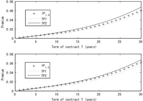
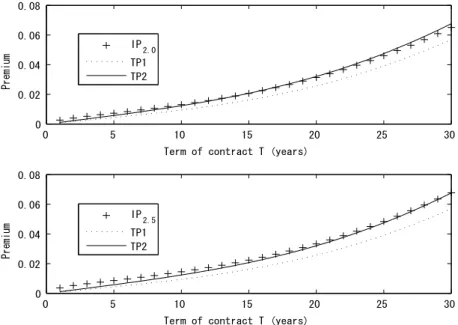
years of term obtained by the traditional pricing methods (1) and (2), respectively. For the valuesa= 1.0, 1.5, 2.0 and 2.5, we denote by IPa(T) the premium of the same contract obtained by the indifference pricing method in Theorem 4.3 with
α(t)≡a. We also write IPfit(T) for the premium of the same contract calculated by the pricing method in Theorem 4.3 withα(t) = 0.6 + 0.36√t, the form of which is chosen to fit the graph of the indifference prices to that of TP2. We used the nonlinear least-squares to determine the form ofα(t) for IPfit(T).
In Figures 4.1–4.3, we plot the graphs of TP1, TP2, IPa, and IPfit. We see that the fitted premiums IPfit(T) simultaneously approximate the corresponding traditional prices TP2(T) well. We have repeated this procedure for various prices and obtained good fits in most cases. This observation suggests the followingimplied utility approach to coherent pricing: insurance companies estimate their implied utility functions by applying this method to existing products, and then refers to them in pricing other products.
0 5 10 15 20 25 30
0 0.02 0.04 0.06 0.08
Term of contract T (years)
Premium
IP
1.0
TP1 TP2
0 5 10 15 20 25 30
0 0.02 0.04 0.06 0.08
Term of contract T (years)
Premium
IP
1.5
TP1 TP2
Figure 4.1. TP1 and TP2 vs. IP1.0 and IP1.5.
References
[1] Acciaio, B. (2007): Optimal risk sharing with non-monotone monetary functionals.Finance Stoch., 11, 267–289.
0 5 10 15 20 25 30 0
0.02 0.04 0.06 0.08
Term of contract T (years)
Premium
IP
2.0
TP1 TP2
0 5 10 15 20 25 30
0 0.02 0.04 0.06 0.08
Term of contract T (years)
Premium
IP
2.5
TP1 TP2
Figure 4.2. TP1 and TP2 vs. IP2.0 and IP2.5.
0 5 10 15 20 25 30
0 0.02 0.04 0.06 0.08
Term of contract T (years)
Premium
IP
3.0
TP1 TP2
0 5 10 15 20 25 30
0 0.02 0.04 0.06 0.08
Term of contract T (years)
Premium
IP
fit
TP1 TP2
Figure 4.3. TP1 and TP2 vs. IP3.0 and IPfit.
[2] Artzner, P., F. Delbaen, J. M. Eber, and D. Heath (1999): Coherent measures of risk.Math. Finance, 9, 203–228.
[3] Barrieu, P. and N. El Karoui (2005): Inf-convolution of risk measures and optimal risk transfer.Finance Stoch., 9, 269–298.
[4] Bielecki, T. R., M. Jeanblanc, and M. Rutkowski (2004): “Hedging of defaultable claims,” in Paris-Princeton lectures on Mathematical Finance 2003, eds. R. Carmona, Berlin: Springer, 1–132.
[5] Borch, K. (1960): Reciprocal reinsurance treaties.ASTIN Bull., 1, 170–191.
[6] Borch, K. (1960): The safety loading of reinsurance premiums. Skand. Aktuarietidskr., 1, 163–184.
[7] Borch, K. (1962): Equilibrium in a reinsurance market.Econometrica, 30, 424–444. [8] B¨uhlmann, H. (1980): An economic premium principle.ASTIN Bull., 11, 52–60. [9] B¨uhlmann, H. (1984): The general economic premium principle.ASTIN Bull., 14, 13–21. [10] B¨uhlmann, H. and W. S. Jewell (1979): Optimal risk exchanges.ASTIN Bull., 10, 243–262. [11] Burgert, C. and L. R¨uschendorf (2006): On the optimal risk allocation problem.Stat. Decis.,
24, 153–171.
[12] Craven, B. D. (1978): Mathematical programming and control theory, London: Chapman & Hall.
[13] Dana, R. -A. and M. Jeanblanc (2003): Financial markets in continuous time, Berlin: Springer.
[14] Dana, R. -A. and M. Scarsini (2007): Optimal risk sharing with background risk. J. Econ. Theory, 133, 152–176.
[15] Delbaen, F. (2002): “Coherent measures of risk on general probability spaces”, inAdvances in Finance and Stochastics, Essays in Honor of Dieter Sondermann, eds. K. Sandmann and P. J. Sch¨onbucher, Berlin: Springer, 1–37.
[16] Duffie, D. (2001): Dynamic asset pricing theory, 3rd. ed., Princeton: Princeton Univ. Press. [17] F¨ollmer, H. and A. Schied (2002): Convex measures of risk and trading constraints.Finance
Stoch., 6, 429–448.
[18] F¨ollmer, H. and A. Schied (2004): Stochastic finance, 2nd ed., Berlin: De Gruyter.
[19] Gerber, H. U. (1978): Pareto-optimal risk exchanges and related decision problems.ASTIN Bull., 10, 25–33.
[20] Gerber, H. U. and G. Pafumi (1998): Utility functions: From risk theory to finance.N. Am. Actuar. J., 2, 74–100.
[21] Heath, D. and H. Ku (2004): Pareto equilibria with coherent measures of risk.Math. Finance, 14, 163–172.
[22] Hodges, S. D. and A. Neuberger (1989): Optimal replication of contingent claims under transaction costs.Rev. Futures Markets, 8, 222–239.
[23] Jouini, E., W. Schachermayer, and N. Touzi (2007): Optimal risk sharing for law invariant monetary utility functions. to appear inMath. Financ.
http://www.fam.tuwien.ac.at/˜wschach/pubs/preprnts/prpr0122.pdf
[24] Musiela, M. and T. Zariphopoulou (2004): An example of indifference prices under exponen-tial preferences.Finance Stoch., 8, 229–239.
[25] Møller, T. and M. Steffensen (2007):Market-valuation methods in life and pension insurance, Cambridge: Cambridge Univ. Press.
[26] Rouge, R. and N. El Karoui (2000): Pricing via utility maximization and entropy. Math. Finance, 10, 259–276.
Japan Credit Rating Agency, Ltd., Jiji Press Building, 5-15-8 Ginza, Chuo-ku, Tokyo 104-0061, Japan
E-mail address:[email protected]
Department of Mathematics, Hokkaido University, Sapporo 060-0810, Japan
E-mail address:[email protected]
Japan Science and Technology Agency, Center for Research in Advanced Financial Technology, Tokyo Institute of Technology, Ookayama 152-8852, Japan
E-mail address:[email protected]