九州大学学術情報リポジトリ
Kyushu University Institutional Repository
周波数が時間に比例して上昇する反射音の生成機構 解明に関する研究
清原, 健司
Graduate School of Design, Kyushu University
https://doi.org/10.15017/25955
出版情報:Kyushu University, 2012, 博士(芸術工学), 論文博士 バージョン:
権利関係:
Analyzing Generation Mechanism of Specific Echoes whose Frequency Increases Linearly with Time
(周波数が時間に比例して上昇する反射音の生成機構解明に関する研究)
Dec 2012 Kenji Kiyohara
清原 健司
Abstract A new phenomenon that we call a sweeping echo is described and investigated. When we clap hands in a regularly shaped reverberant room, we hear sweeping echoes whose frequency increases linearly with time. An example of sweeping echoes observed in a rectangular reverberation room is first described. Then, the mechanism that generated the sweeping echoes is investigated by assuming a cubic room and using number theory. The reflected pulse sound train is found to have almost equal intervals between pulses on the squared-time axis.
This regularity of arrival times of the reflected pulse sounds is shown to generate the weeping echoes. Computer simulation of room acoustics shows good agreement with theoretical results.
Next, we investigated sweeping echoes in a two-dimensional
(2D) space. We first describe our investigation of a square
cross-section based on number theory. Next, we describe
rectangular cross-section with various aspect ratio investigated
based on the same theory as that for the square. We also discuss
our measurements of sweeping echoes in a long hallway. We
propose a method for extracting sweep rates of sweeping echoes
Acknowledgements
I would like to express my gratitude to my supervisor, Associate Professor Akira Omoto of Kyushu University.
I am very thankful to Professor Shin’ichiro Iwamiya and Associate Professor Toshiya Samejima of Kyushu University for useful advices.
I would also like to thank Professor Yutaka Kaneda of Tokyo Denki University for giving me a chance to research this work.
I am very thankful to my superior Professor Ken’ichi Furuya of Oita University for giving me a lot of useful advice.
I would also like to thank my colleagues for helping me this work.
Contents
Acknowledgements i Contents ii I. Introduction 1 II. Sweeping echoes perceived in a rectangular parallelepiped
reverberation room 4
II.1 Measured sweeping echoes 4
A. Measurement conditions and sweeping echoes 4 B. Time-frequency analysis of the sweeping echoes 6 II.2 Generation mechanism of the main sweeping echo (cubic room) 8
A. Intervals of reflected sounds in a cubic room 8 B. Relationship between the squared-time axis and time axis 11
C. Main sweeping echo 12
II.3 Generation mechanism of the sub-sweeping echoes
(Influence of the forbidden numbers) 14
II.4 Numerical simulation 16
III. Examination on the Three Dimensional Case 22 III.1 Auto-correlation of the measured data 22 III.2 Recommended volume of the reverberation room 26 III.3 Conclusion of sweeping echoes in 3D spaces 27 IV. Sweeping echoes in a two-dimensional space
(square cross-section) 28
IV.1 Generation mechanism of main sweeping echo in 2D space 29 IV.2 Sub-sweeping echoes (Effect of forbidden numbers) 32
IV.4 Experiment 37 V. Examination on the Two Dimensional Case 42 V.1 Method for extracting sweep sound 42 A. Complex ascending sweep sine signal 42 B. Correlation results with sweeping echoes 45 V.2 Forbidden numbers of rectangular cross-section 48
A. Formulation 48
B. Examples 50
C. Cases that a2 is a rational number 52 D. Case that a2 is an irrational number 54 V.3 Conclusion for sweeping echoes in 2D spaces 55
VI. Conclusion 57
References 59
Appendix A. Forbidden numbers for sum of three square numbers 61 Appendix B The ratio of forbidden numbers for all positive integers 62
I. INTRODUCTION
A new, interesting acoustical phenomenon is described, and its generation mechanism is investigated theoretically.
When we clap hands once between parallel hard walls, we hear a sound called “fluttering echo.”[1]. A single handclap sound (i.e., an impulsive sound) is reflected by the walls repeatedly, and a train of pulses with periodic intervals is generated. This pulse train causes a specific sound sensation;
that is, a fluttering echo.
In the fluttering echo, reflected sounds go forward and backward in a one-dimensional pattern between parallel hard walls. What happens, then, when we clap hands in a three-dimensional (3D) reflective space? The author found sweep sound (Audio illustrations are available at:
http://www.asp.c.dendai.ac.jp/sweep/) which the author call “sweeping echoes,” were perceived when we generated a pulse sound in a regularly shaped reverberation room. The perceived frequency of the sweep sounds increased with time at different speeds. Other researchers have also noticed the sweeping echoes in squash courts, which also had hard regularly shaped walls.
ISO [2] allows rectangular reverberation room because of its construction cost and easiness of measurement. Also Japanese Industrial Standard (JIS)
There are some other types of sweeping (or sliding) echoes. One is caused by frequency dispersion. The frequency dispersion assumes some special sound field where the phase velocity of a sound varies with its frequency. This is not the case here; the sweeping echoes presented in this paper occur in normal sound field, without dispersion.
Knudsen[4] reported another type of frequency shift in reverberated sound.
He reported that the pitch of a tone in a small, resonant room might change perceptively during the decay of the tone. The pitch of the emitted sound is considered to be changed to that of a resonance frequency. On the other hand, our sweeping echoes are clearly explained in the time domain based on the number theory.
Kaneda et al [5] reported when a stone is dropped in a circular long pipe (about 100m length, 20cm diameter), sweep sounds whose frequency decreases with time are observed and they analyzed its generation mechanism.
Another researcher noticed when a handclap is once occurred toward a flight of steps (about 40m width, 25 steps), echoes whose frequency varies with time are perceived.
Sweep component often appears when measuring an impulse response using TSP signal. However, this is not sweeping echoes but the harmonic distortion of the loudspeaker [6].
In this paper, the sweeping echoes observed in a rectangular parallelepiped reverberation room are described first with their time-frequency analysis in Sec. II. 1. Then, the generation mechanism of the sweeping echoes in a cubic
theoretical results are compared with simulation results in Sec. II. 4.
Section III describes Examination on the Three Dimensional Case. Sec. III.1 discusses sweeping echoes in a rectangular parallelepiped reverberation room by auto-correlation of the measured data. Sec. III.2 considers an adequate volume of the reverberation room. Sec. III.3 concludes sweeping echoes in 3D spaces.
Sec. IV describes sweeping echoes in a two-dimensional (2D) space (square cross-section) and discusses whether the above theory can be applied to a 2D space and theoretically analyzes the generation mechanism of the echo.
Section IV.1 describes the main sweeping echo based on the above research.
Section IV.2 describes sub-sweeping echoes in 2D spaces. Section IV.3 shows a numerical simulated result. Section IV.4 describes an experiment result and compares with the theoretical result.
In Section V, Examination on the Two Dimensional Case is described. Sec.
V.1 proposes a new method for detecting sweeping echoes and the theoretical and experimental results for sweeping echoes are confirmed.
Sec. V.2 describes forbidden numbers of rectangular cross-section. Sec. V.3 concludes sweeping echoes in 2D spaces.
Section VI concludes the paper.
II. SWEEPING ECHOES PERCEIVED IN A RECTANGULAR PARALELEPIPED REVERVERATION ROOM
Sweeping echoes are perceived in relatively large, regularly shaped three-dimensional rooms with highly reflective surfaces; i.e., walls, ceiling, and floor. The author first describes the sweeping echoes measured in a rectangular parallelepiped reverberation room along with time-frequency analysis.
II. 1 Measured sweeping echoes
A. Measurement conditions and sweeping echoes
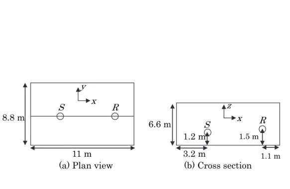
The dimensions of the rectangular parallelepiped reverberation room were 11 m (width) × 8.8 m (depth) × 6.6 m (height) [7]. The measurement conditions are shown in Fig. 2.1. Figures 2.1(a) and (b) show the plan view and cross section of the reverberation room, respectively. The symbols S and R represent the source and reception positions, respectively. As shown in Fig.
2.1(a), both S and R were located on the center line of the floor. S was located 3.2 m from the wall and 1.2 m high, and R was 1.1 m from the opposite wall and 1.5 m high as shown in the figure, respectively.
When hands were clapped once at position S, the first sweep sound whose frequency increases over a short time (called the main sweeping echo) was perceived at position R. Multiple sweep sounds whose frequency increased relatively slowly (called sub-sweeping echoes) were then perceived, along with ordinary reverberation sounds.
Although sweep sounds were perceived at other source and reception
symmetrical with respect to the room, such as those shown in Fig. 2.1. To analyze these sweep sounds, they were recorded with a microphone placed at position R.
(a) Plan view (b) Cross section
FIG. 2.1 Layout for sweep-sound measurement. (a) Plan view, (b) cross section. S, source position, R, reception position.
11 m
8.8 m S R x
y
6.6 m S x R
1.2 m 1.5 m
z
3.2 m 1.1 m
B. Time-frequency analysis of the sweeping echoes
Figure 2.2 shows the results of analyzing the recorded echoes by using short-time Fourier transformation. The horizontal axis represents time, and the time when hands were clapped is set to the origin. The figure shows the spectrogram for the first 2seconds. The vertical axis represents frequency, up to 2 kHz, which was the range within which the sweep sounds clearly perceived. The analysis conditions were the following: the sampling frequency was 16 kHz, a 16-ms rectangular window (62.5 Hz frequency resolution) was used, and the window was shifted in steps of 8 ms.
In Fig. 2.2, the main sweeping echo appears clearly from 0 to about 400 ms [line (A)]. The frequency of the main sweeping echo increased linearly with time, and it rose to about 1500 Hz during the first 400 ms. This result corresponds with hearing perception. Following the main sweeping echo, multiple sub-sweeping echoes whose frequency rose linearly at relatively slow speeds, also appear in Fig. 2.2.
0 0.2 0.4 0.6 0.8 1 1.2 1.4 1.6 1.8 2 0
200 400 600 800 1000 1200 1400 1600 1800 2000
Time
Frequency (Hz)
-60 -40 -20 0 20 40
FIG. 2.2 Spectrogram of the recorded data. The main sweeping echo appears clearly from 0 to about 400 ms [line (A)]. The frequency of the main sweeping echo increased linearly with time, and it rose to about 1500 Hz during the first 400 ms. Following the main sweeping echo, multiple sub-sweeping echoes also appeared whose frequency rose linearly at relatively slow speeds.
[s]
Relative Level [dB]
(A) Main sweeping echo
II.2 Generation mechanism of the main sweeping echo (cubic room)
In this section, the author investigates the generation mechanism of the main sweeping echo, based on geometrical acoustics and number theory. As the first step in this investigation, a cubic room is assumed in this paper.
A. Intervals of reflected sounds in a cubic room
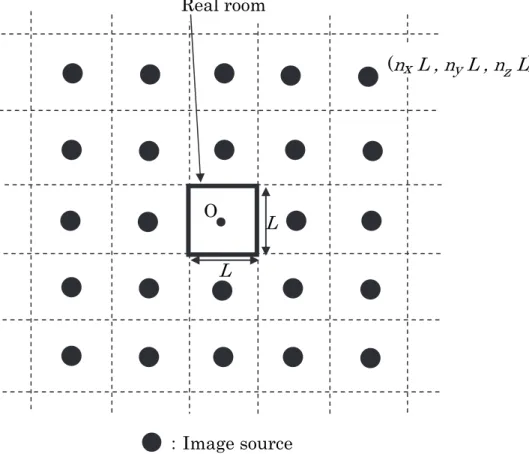
First, the regularity of arrival time of reflected sounds in a cubic room is described. To simplify the issue, the source and reception points are both assumed to be located at the center of the room. Figure 2.3 shows the mirror image sources generated in a cubic room based on geometrical acoustics [8].
The figure shows a top view, and the edge length of the room is denoted by L. When a pulse sound is generated at the center of the room, the arrival times and amplitude of the observed reflected sounds are the same as those of the sounds that would be generated from the image sources shown in Fig. 2.3. In other words, the reflected sounds can be treated as the sounds from the image sources.
The coordinate origin O is set at the center of the room. Then, the location of each image source is represented by (nxL, nyL, nzL), where nx, ny, nz are integers. The distance d between the origin (reception position) and an image source of (nxL, nyL, nzL) is represented by
d
n
xL
2 n
yL
2 n
zL
2 n
x2n
y2n
z2L. (2.1)Thus, the arrival time of the sound from the image sources is obtained by dividing d by sound velocity c, as in the following equation:
FIG. 2.3 Mirror image sources of a cubic room. The figure shows a top view, and the size of the room is denoted by L. The reflected sounds are treated as the sounds from the image sources. The coordinate origin O is set to the center of the room. The location of each image source is represented by (nxL, nyL, nzL), where nx, ny, nz are positive and negative integers.
O
L L Real room
(nx L , ny L , nz L)
:Image source
. .
/ 2 2 2
c
L y z
c x d
d
n n n
(2.2)Next, consider the arrival time on the squared-time axis. The squared arrival time is derived by squaring Eq. (2.2):
t
2n
x2n
y2n
z2
Lc 2M Lc 2, (2.3)M
n
x2n
y2n
z2. (2.4)Thus, the squared arrival time t2 is represented by an integer M times a constant (L/c)2. Equation (2.3) represents the position on the squared-time axis at which the reflected sound exists.
From number theory [9], the sum of the squared integers
n
x n
y n
z2 2 2
expresses all integers, except the “forbidden numbers,” i.e.,
M ≠ 4k(8m+7), (2.5)
where k, m = 0, 1 , 2, …. (Appendix A).
Since these forbidden numbers account for 1/6 of all positive integers (Appendix B), the author first disregards the forbidden numbers and assume that M includes approximately all positive integers. Then Eq. (2.3) indicates that reflected sounds (pulse sounds) exist (L/c)2, 2(L/c)2, 3(L/c)2,…; that is, they exist at equal intervals of (L/c)2 on the square-time axis.
B. Relationship between the squared-time axis and the time axis
The author represents the arrival times of two adjacent pulses (reflected sounds) as ta and tb (ta < tb). The interval between these pulses on the squared-time axis is (L/c)2. Namely
Lct tb a
2 2
2 . (2.6)
By factoring the left-hand side of Eq. (2.6), we obtain
tbta
tbta
Lc 2. (2.7)The average arrival time tv of the two pulses is defined by
tv=( tb + ta)/2. (2.8)
By substituting Eq.(2.8) into Eq. (2.7) and modifying it, the interval between pulses on the time axis represented by the following equation:
c t
t L t
v a
b
1 2 2
2 . (2.9)
Equation (2.9) clarifies that the interval between the two pulses is inversely proportional to the time tv.
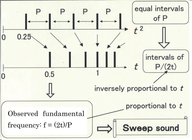
Thus, a pulse series with equal intervals on the squared-time axis has intervals inversely proportional to time on the time axis. Figure 2.4 illustrates this relationship.
C. Main sweeping echo
A periodic pulse series has a fundamental frequency represented by the reciprocal of its interval [10]. Therefore, when the interval of pulses is represented by Eq. (2.9), the fundamental frequency of the pulses at time tv
is expressed by the following equation:
2 (2.10)) 1
( 22 t
L c t
f t v
a v b
t
Equation (2.10) indicates that the fundamental frequency f is proportional to the time tv. In other words, human perceive an increasing sweep sound.
This proves that a reflective pulse train in a cubic room produces a sweep sound sensation.
FIG. 2.4 A pulse series with equal intervals on the squared-time axis has intervals inversely proportional to time on the time axis.
Observed fundamental
frequency: f = (2t)/P
II. 3 Generation mechanism of the sub-sweeping echoes (Influence of the forbidden numbers)
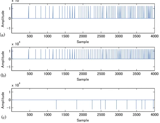
As described above, a pulse series from the image sources of a cubic room does not have completely equal intervals on the squared-time axis because of the forbidden numbers. The influence of the forbidden numbers can be explained as the addition of a forbidden numbers pulse train which has pulses corresponding to forbidden numbers on the squared-time axis with negative amplitudes. Figure 2.5 conceptually illustrates this phenomenon.
Figure 2.5(a) shows a pulse series on the time axis of a cubic room for equal amplitudes, where the dimension L of the cubic room was assumed 10 m.
Some pulses are missing because of the forbidden numbers. These gaps were considered to be generated by adding a pulse series corresponding to the forbidden numbers with negative amplitude of the same values [Fig. 2.5(c)]
to a pulse series with completely equal intervals on the squared-time axis [Fig. 2.5(b)].
From Eqs. (2.3) and (2.5), the squared arrival time for the pulse series corresponding to the forbidden numbers is represented by the following equation:
Lct k m
2
24 (8 7) , (2.11)
where k, m=0, 1, 2, 3, … .
The pulse series has equal intervals of 4k8(L/c)2, for k=0, 1, 2, … , on the squared-time axis as m changes. For a typical example, corresponding to k=0, m=0, 1, 2, … , the period of the pulse series becomes 8(L/c)2. The
500 1000 1500 2000 2500 3000 3500 4000 -1
0 1
x 104
Sample
Amplitude
500 1000 1500 2000 2500 3000 3500 4000
-1 0 1
x 104
Sample
Amplitude
500 1000 1500 2000 2500 3000 3500 4000
-1 0 1
x 104
Sample
Amplitude
FIG. 2.5 The influence of the forbidden numbers. (a) A pulse series on the time axis of a cubic room for equal amplitudes. (b) A pulse series with completely equal intervals on the squared-time axis. (c) A pulse series corresponding to the forbidden numbers with the negative amplitude of the same values. The gaps of (a) are considered to be generated by adding (c) to
(a)
(b)
(c)
corresponding to this example is represented by the following equation:
fb(
t
v)
2Lc22 81tv. (2.12)For k=1 and m=0, 1, 2, … , the period of the pulses becomes 32(L/c)2, and its fundamental frequency is represented by the following equation:
fb(
t
v)
2Lc22 321 tv. (2.13)For k=2, 3, 4, … , the fundamental frequency is represented in a similar way.
The pulses series corresponding to the forbidden numbers thus consists of multiple pulse series with different periods on the squared-time axis. Since these periods are longer than that of the main sweeping echo, the fundamental frequencies of the pulse series corresponding to the forbidden numbers increase more slowly. Thus, sub-sweeping echoes are generated.
II.4 Numerical simulation
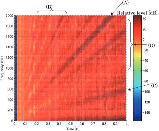
The theoretical results derived in the preceding sections were confirmed by time-frequency analysis. Figure 2.6(a) shows the spectrogram of the pulse series shown in Fig. 2.5(b). The spectrogram was calculated by FFT with a 16-ms rectangular time window and an 8-ms shift. In Fig. 2.6(a), the main sweeping echo (A) appears clearly. The lines (B) are its harmonics.
Calculating the slope (or frequency rising speed, or sweep speed) of the main sweeping echo from Eq. (2.10) with sound velocity c=340 m/s gave 2c2/L2 =2312 Hz/s. This value is consistent with the slope of the main
0 0.1 0.2 0.3 0.4 0.5 0.6 0.7 0.8 0.9 1 0
200 400 600 800 1000 1200 1400 1600 1800 2000
Time
Frequency (Hz)
-150 -100 -50 0 50
0 0.1 0.2 0.3 0.4 0.5 0.6 0.7 0.8 0.9 1
0 200 400 600 800 1000 1200 1400 1600 1800 2000
Frequency (Hz)
-150 -100 -50 0 50
(a)
(b)
Relative level [dB]
Relative level [dB]
(B) (A)
(C) (D) [s]
Figure 2.6(b) shows the spectrogram of the pulse series shown in Fig. 2.5(c).
The sub-sweeping echo (C) corresponding to k=0 appears clearly, and its harmonics (D) also appear. Calculating the slope of the sub-sweeping echo for k=0 from Eq. (2.12) gave (2c2/L2)/8=289 Hz/s. This value is consistent with the slope of the sub-sweeping echo (C) shown in Fig. 2.6(c).
Figure 2.7 shows the spectrogram of the pulse series shown in Fig. 2.5(a).
The spectrogram is almost the power sum of the spectra shown in Fig. 2.6(a) and (b). The main sweeping echo (A) and its harmonics (B), and the sub-sweeping echo (C) corresponding k=0 and its harmonics (D) all appear in Fig. 2.7. Thus, the main sweeping echo and the sub-sweeping echoes corresponding to the forbidden numbers were perceived for the pulse series shown in Fig. 2.5(a).
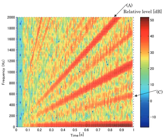
Next, the reflected sounds of a pulse sound (i.e., an impulse response) in the cubic room were simulated by the mirror image method [11]. Dimension L for the room was 10 m. The calculated reflected pulses were convolved with a sinc function and overlap added [12] to derive sampling data. Figure 2.8 shows the spectrogram of the simulated sounds. Multiple sweep sounds appear, and just as in Fig. 2.7, the main sweeping echo (A) appears clearly.
The sub-sweeping echo (C) also appears.
Since the sound source and reception point were located at the center of the room, different numbers of multiply reflected pulses arrived at the same time due to degeneracy of the mirror image sources. Therefore, the amplitudes of the reflected-pulse series were not equal. This caused random noisy spectrum that was superposed on the time-spectrum plot. As a result,
0 0.1 0.2 0.3 0.4 0.5 0.6 0.7 0.8 0.9 1 0
200 400 600 800 1000 1200 1400 1600 1800 2000
Time
Frequency (Hz)
-140 -120 -100 -80 -60 -40 -20 0 20 40
FIG. 2.7 Spectrogram of the pulse series shown in Fig. 2.5(a). The spectrogram is almost the power sum of the spectra shown in Figs. 2.6(a) and (b). The main sweeping echo (A) and its harmonics (B), and the sub-sweeping echo (C) and its harmonics (D) all appear.
Relative level [dB]
(B) (A)
(C) (D)
[s]
0 0.1 0.2 0.3 0.4 0.5 0.6 0.7 0.8 0.9 1 0
200 400 600 800 1000 1200 1400 1600 1800 2000
Time
Frequency (Hz)
-10 0 10 20 30 40 50
FIG. 2.8 Spectrogram of the impulse response in a cubic reverberation room whose dimension L is 10 m. Multiple sweep sounds appear, and just as in Fig.
2.7, the main sweeping echo (A) appear clearly. The sub-sweeping echo (C) also appears.
Relative level [dB]
[s]
(A)
(C)
same sweeping echoes shown in Fig. 2.7 can also be recognized in Fig. 2.8.
The slopes of lines (A) and (C) in Fig. 2.8 are similar to the theoretical values 2312 Hz/s and 289 Hz/s, respectively, calculated above. Thus, the theoretical results developed in the preceding section adequately explain the sweeping echo phenomenon that appeared in the computer simulation of room acoustics.
III. Examination on the Three Dimensional Case III.1 Auto-correlation of the measured data
Unlike a cubic room, all the side lengths of a rectangular parallelepiped room are not equal. Therefore, the arrival time of a reflected sound from image source cannot be represented by a simple formula like Eq. (2.2). This makes theoretical analysis using number theory difficult.
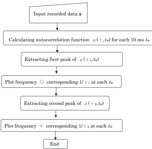
Therefore, the author attempted a qualitative explanation by analyzing experimental data. A pulse sound was generated by hand clapping under the conditions shown in Fig. 2.1. Then, the periodicity of the received pulse train (reverberation sound) was studied based on the short-time autocorrelation method. The short-time autocorrelation function ρ(τ, tw) was calculated from the windowed data centered at time tw, and it was calculated repeatedly with sliding time tw. The sampling frequency was 16 kHz, and the window length was 10 ms.
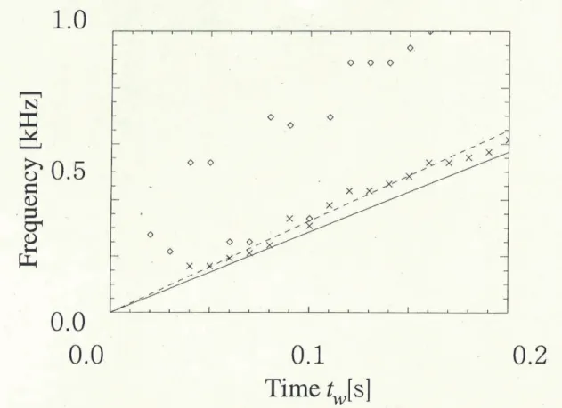
When the reflected pulses contain periodic pulses, the autocorrelation functionρ(τ, tw), as a function of time τ with fixed tw, has peaks at times, τ s, corresponding to the pulse periods. These peak times, or pulse periods were calculated as a function of tw. The results are shown in Fig. 3.1, as the reciprocals of the detected periods, which correspond to the frequencies. Fig.
3.2 shows a flowchart for calculating the frequencies.
In Fig. 3.1, the horizontal axis represents the time tw and the vertical axis represents the reciprocal of the peak of the autocorrelation function by frequency. The ♢ symbol denotes the frequencies that correspond to the first high peaks ofρ(τ, tw) for each tw, and the × symbol denotes the
The root-mean-square Lm of the side lengths of the rectangular parallelepiped room was calculated using the following equation:
Lm
Lx2L2yL2z
/3. (3.1)Substituting the dimension of the experimental room (Lx=11 m, Ly=8.8m, Lz=6.6 m from Fig.1) gave Lm=8.98 m. A function derived by substituting Lm
into Eq. (2.10), representing the theoretical frequency of a main sweeping echo for a cubic room with side length of Lm, is shown as a solid line in Fig.
3.1. This solid line is close to the ×. The line of the main sweeping echo observed in Fig. 2.2 is also plotted in Fig. 3.1, by a broken line, and it is also close to the theoretical line plot.
This result indicates that the calculated frequency line of a sweeping echo based on Lm matches the observed sweeping echo, and its sweeping frequency corresponds to the periodicity in the pulse train appearing as the second high peak of the short-time autocorrelation function. It is left for future study to answer the question why the second high peaks but not the first ones, and what do the first high peaks represent.
FIG. 3.1 Reciprocal of peak time of short-time autocorrelation ρ(τ) of recorded data shown in Fig. 2.2. ♢, the first high peak ofρ(τ). ×, the second high peak ofρ(τ). Solid line, theoretical frequency. The solid line is closed to the × symbols. Broken line, the line of main sweeping echo observed in Fig. 2.2. It is also close to the theoretical line plot.
Thus, the main sweeping echo in a rectangular parallelepiped room has reflected pulse periods close to those of a cubic room with the same mean side length Lm as the rectangular parallelepiped room. This implies that the pulse train in a rectangular parallelepiped room has a regularity similar to that in a cubic room, and this regularity causes sweeping sounds.
FIG. 3.2 Flowchart for calculating frequencies corresponding to reflected pulse series.
Input recorded data x
Calculating autocorrelation function ρ(τ,tw) for each 10 ms tw
Extracting first peak of ρ(τ1,tw)
Plot frequency ◇ corresponding 1/τ1 at each tw
Extracting second peak of ρ(τ2,tw)
Plot frequency × corresponding 1/τ2 at each tw End
III.2 Recommended volume of the reverberation room Eq. (3.2) indicates modified Eq. (2.10) for Lm instead of L;
2 (3.2))
( 22 t
L
f c v
v m
t
The smaller Lm is, the more quickly f (tv) increases. ISO [2] allows rectangular reverberation room because of its construction cost and easiness of measurement. Also Japanese Industrial Standard (JIS) [3] recently allowed the rectangular shaped reverberation room as TYPE II room. ISO [2]
prescripts the volume of the reverberation shall be at least 150 m3 corresponding to about Lm = 5.5 m. Then, f (tv=1 s) = 7643.0 Hz. This frequency can be difficult to be perceived. The size of our previous reverberation room was 11 m×8.8 m×6.6m, i.e. its volume was 638.88 ㎥.
The Lmin Eq. (3.2) was about 8.6 m and f (tv=1 s) = 3116.8 Hz. The frequency is easy to be perceived, therefore, such huge size should be avoided for acoustical measurements.
Our reverberation room was reconstructed as decreasing the volume 1/3, about 200 m3. In the room, the sweeping echo is difficult to be perceived. ISO [2] strongly recommend the volume to be at least 200 m3, but not greater than 500 m3 because of air absorption at high frequencies.
Therefore, the recommended volume seems to be about 200 m3 to avoid acoustic cumbrance by the sweeping echoes.
III.3 Conclusion of sweeping echoes in 3D spaces
When a pulse sound is generated in a rectangular parallelepiped reverberation room, a peculiar phenomenon is observed in that the frequency components of the reflected sounds increase linearly (called “sweeping echoes”). These sweeping echoes consist of a “main sweeping echo,” whose frequency component increases over a short time, and “sub-sweeping echoes,” whose frequency components increase slowly. Investigating the sweeping echoes assuming a cubic room showed that the arrival times of the pulse sounds from mirror image sources had almost equal intervals on the squared-time axis, and this regularity of the pulse intervals generated the main sweeping echo. The pulse train does not have exactly equal intervals on the squared-time axis, but rather has some missing pulses corresponding to
“forbidden numbers” based on number theory. These missing pulses were shown to have relatively long, equal intervals. This regularity causes the sub-sweeping echoes. Computer simulation based on the image method produced results in good agreement with the theoretical results.
IV. SWEEPING ECHOES IN A 2D SPACE (square cross-section)
The author focuses on the sweep echo phenomenon in a 2D space. Section IV.1 discusses whether our proposed theory in Sec. II can be applied to a 2D space and theoretically analyzes the generation mechanism of the echo. The author first discusses a square cross-section.Section IV.1 describes the main sweeping echo based on our above research. Section IV.2 describes sub-sweeping echoes in square cross-section. Section IV.3 shows simulation results and compares them with the theoretical results. Section IV.4 shows the experimental results and compares them with the theoretical and simulation results.
The author analyzed the sweeping echoes for a source and receiver at the center of a cross-section. The sweeping echoes were not only perceived at the exact center position but also around the center.
IV.1 Generation mechanism of main sweeping echo in 2D space
Figure 4.1 shows a sound source and its mirror image sources generated in a rectangular cross-section field based on geometrical acoustics [8]. The size of the square space is denoted by L×L, where L is positive real number. The reflected sounds can be treated as sounds from the mirror image sources.
FIG. 4.1 Mirror image sources of rectangular cross-section field. Coordinate : Image source
O
L L Real space
Source
(nxL, nyL)
The sound source and reception point are located at the center of the rectangular space. The coordinate origin O is also set at the center of the space. The location of each image source is then represented by (nxL, nyL), where nx and ny are positive or negative integers. The distance d between the origin and an image source of (nxL, nyL) is represented by
.
) ) (
(
2 2 2 2
n n n n
x y
L L L
d x y
(4.1)
The arrival time of the sound from the image source is obtained by dividing d by the velocity of sound c, as in the following equation:
.
/
2 2
c L c
d t
n
xn
y(4.2)
Next, consider the arrival time on the ‘squared-time axis’, which is derived by squaring Eq. (4.2):
2 2 2 2 2
c q L
c
n L
n
t x y
, (4.3)
where
qnx2ny2. (4.4)
q becomes an integer for all nx and ny. Now, assume q takes all positive integers when nx and ny take all integers; however, this does not happen in actuality, as stated in Sec. IV.2. However, to simplify, assume that the squared arrival time t2 in Eq. (4.3) has an equal interval (L/c)2.
Considering that a sound source emits a sound pulse, the author represent
The interval between these pulses on the squared-time axis is (L/c)2. Namely,
2 2
2
c
t
Lt
b a . (4.5)By factoring the left-hand side of Eq. (4.5), we obtain
c
t L t t
t
b a b a2
) )
(
(
. (4.6)The mean arrival time tv of the two pulses is defined by tv=( tb + ta)/2 . (4.7)
By substituting Eq. (4.7) into Eq. (4.6) and modifying the resultant equation, the interval between pulses on the time axis is represented by the following equation:
t t
t
v a
b c
L 1
2 2
2 . (4.8)
A periodic pulse series has a fundamental frequency represented by the reciprocal of its interval [10]. Therefore, when the interval of pulses is represented by Eq. (4.8), the fundamental frequency of the pulses at time tv
is expressed by the following equation:
t t t t
va b
v L
f c
1 222 )
( . (4.9)
Equation (4.9) indicates that the fundamental frequency f (tv) of the reflected
IV.2 Sub-sweeping echoes (Effect of forbidden numbers)
Number theory states that q in Eq. (4.4) can take the most positive integers but does not take specific positive integer values, which are called “forbidden numbers” [9]. This section describes the effect of these forbidden numbers.
The forbidden numbers are expressed as follows [13]:
q≠k2r (4h + 3) , (4.10)
where k, r, h = 0, 1, 2, …,and all squared factors of q are included in k2 not in r (4h + 3), and r≠4h + 3.
The forbidden numbers correspond to absent pulses, which are caused by pulses added in anti-phase to all integers. Figure 4.2 (b) shows a pulse series that has completely equal intervals on the squared-time axis, where L = 4 m.
Figure 4.2 (a) shows an equal amplitude pulse series of a square cross- section field, which lacks pulses due to forbidden numbers. Figure 4.2 (c) shows an anti-phased pulse series corresponding to forbidden numbers, where the amplitudes are normalized as 1. Clearly, Fig. 4.2 (b) added to Fig.
4.2 (c) becomes Fig. 4.2 (a).
For k =r = 1, substituting Eq. (4.10) into Eq. (4.3) gives
2
2 (4 3)
c
h L
t . (4.11)
Since Eq. (4.11) represents pulse arrival times for h = 0, 1, 2, …, adjacent pulses have interval 4(L /c)2 on the squared-time axis. Therefore, the interval of the anti-phased pulse is 4 times longer than that of Eq. (4.8), and thus its fundamental frequency is 1/4 that of Eq. (4.9), the fundamental frequency of the main sweeping echo. This phenomenon is called “sub-sweeping echo”. For
200 400 600 800 1000 1200 1400 1600 -2
-1 0 1 2
Amplitude
200 400 600 800 1000 1200 1400 1600
-2 -1 0 1 2
Amplitude
200 400 600 800 1000 1200 1400 1600
-2 -1 0 1 2
Amplitude
FIG. 4.2 Effect of forbidden numbers. (a) Pulse series on time axis of square cross-section for equal amplitudes. (b) Pulse with completely equal intervals on squared-time axis. (c) Pulse series corresponding to forbidden numbers with negative amplitude of same values. Gaps of (a) are considered to be
Sample (a)
(b)
(c)
tv= 1 s is 3,612 Hz.
Thus, the forbidden numbers cause a regularity in the lack of reflected pulses and this regularity causes sub-sweeping echoes, i.e., echoes with a small frequency sweep rate.
The forbidden numbers indicate that integers are impossible. This means that a reflected sound pulse does not exist at the time corresponding to the forbidden numbers on the squared-time axis
IV.3 Numerical simulation
In this section, the author confirms, using numerical simulation, the theoretical results of the sweeping echoes described in Section IV.1 and 2.
Echo simulation based on the mirror image method [11] was conducted assuming a 4 × 4 m 2D space. The band-limited impulse response, or echo series, was calculated by convolving echo pulses with a discrete sinc function.
The sampling frequency was 40 kHz. The spectrogram of the impulse response was calculated with a 16-ms Hanning window (62.5-Hz frequency resolution), and the window was shifted in steps of 8 ms.
Figure 4.3 shows the spectrogram of the impulse response. Multiple sweep sounds, whose frequency components linearly increase with time, can be observed. The main sweeping echo (A) can be clearly observed, and the sub-sweeping echo (B) also can be observed. Other sweeping components are harmonics of the main- and sub-sweeping echoes.
The slopes of lines (A) and (B) in Fig. 4.3 are 14,378 and 3,598 Hz/s, respectively, which are almost consistent with the theoretical values of 14,450 and 3,612 Hz/s, respectively, calculated above. Thus, the theoretical results discussed in the previous section clearly explain the sweeping echo phenomenon that appeared in the computer simulation of room acoustics.
The theoretical and numerical models are based on the same mirror-images.
0.1 0.2 0.3 0.4 0.5 0.6 0.7 0.8 0.9 0
0.2 0.4 0.6 0.8 1 1.2 1.4 1.6 1.8
2x 10⁴
Time
Frequency (Hz)
-60 -50 -40 -30 -20 -10 0 10 20 30
FIG. 4.3 Spectrogram of simulated impulse-response in two-dimensional square space. Multiple sweep sounds can be observed, and main sweeping echo (A) can be clearly observed. Sub-sweeping echo (B) also can be observed.
Relative level [dB]
(A)
(B)
[s]
IV.4 Experiment
There are sound spaces that can be regarded as 2D sound spaces. A typical example is a long, straight hallway. A pulse sound generated in such a hallway is reflected repeatedly in the hallway’s cross-section, i.e., 2D space.
Strictly speaking, the cross-section is not a 2D sound space but a 2D subspace of a 3D sound space. In this subspace, however, the arrival time of the reflected pulses is equivalent to that in a 2D sound space. Therefore, the author regards this subspace as a 2D sound space.
However, in practice, 2D sweeping echoes are hardly ever observed, whereas 3D ones can be observed in certain situations. The main reason is that the number of image sources is much smaller in a 2D space than in a 3D space, so the reflected energy is small in a 2D space.
By chance, the author found actual sweeping echoes in a hallway at the Tokyo International Forum, at Yurakucho in Tokyo. The cross-section of the hallway is square with 4-m sides, as shown in Fig. 4.4 (a). The lateral walls are glass plates, which reflect sound well. The hallway is a 40-m-long straight square pipe, with no junctions or doors except at the end. This seems to be a good example of a 2D sound space.
The author measured and analyzed the sweeping echoes generated in this hallway. The measurement conditions are shown in Fig. 4.4 (b). The symbols
FIG. 4.4 Layout for sweep-sound measurement. (a) Dimensions and (b) cross-section, S: source position; R: receiver position.
When a pulse sound (handclap) was generated at position S, sweep sounds whose frequencies increased relatively slowly were perceived, along with ordinary reverberation sounds.
To analyze these sweeping echoes, the author recorded impulse response with a microphone placed at position R and a loudspeaker placed at position S emitting a maximum-length (M-)sequence signal. Figure 4.5(a), (b) shows the recorded impulse-response and the spectrogram of the impulse response, respectively. The horizontal axis represents time; the time when the pulse sound was generated was set to the origin. The vertical axis represents frequency up to 4 kHz, which was the band within which the sweep sounds
4 m
4 m
40 m
4 m
S, R
(a) (b) 4 m
frequency was 16 kHz, a 256-sample rectangular window was used for discrete Fourier transform (DFT), and the window was shifted by 128 samples.
0 0.1 0.2 0.3 0.4 0.5 0.6 0.7 0.8 0.9 1
-3 -2 -1 0 1 2 3x 10⁴
Time [s]
Amplitude
FIG. 4.5(a) Recorded impulse-response. Sampling frequency is 16kHz.
Relative level [dB]
0 0.1 0.2 0.3 0.4 0.5 0.6 0.7 0.8 0.9 1
0 500 1000 1500 2000 2500 3000 3500 4000
Time
Frequency (Hz)
-60 -40 -20 0 20 40
FIG. 4.5(b) Spectrogram of recorded data. Main sweeping echo (A) vaguely appears from 0 to about 0.2 s. Frequency of main sweeping echo increased linearly with time and increased to about 2,200 Hz during first 0.2 s.
Following main sweeping echo, sub-sweeping echo (B) also appears with slope of about 3,500 Hz/s.
7000
0 10
(B) (A)
[s]
In Fig. 4.5(b), a sub-sweeping echo whose frequency increases linearly with time can be seen (Line (B)). The slope of the sub-sweeping echo in Fig. 4.5 is about 3,500 Hz/s, which is in good agreement with the theoretical 3,612 Hz/s calculated by Eq. (4.9).
Compared with the simulation results in Fig. 4.3, the sub-sweeping echo in Fig. 4.5 is not clear. There are two main reasons for this lack of clarity. First, the reflection coefficient was set to 1 in the simulation, while the mean pressure reflection coefficient of the experimental space was about 0.9, determined using numerical simulation. Generally, in a real space, the higher the frequency, the lower the reflection coefficient, which means low-frequency reverberance. This causes fast decay of the high-frequency components of sweeping echoes. Sweeping echoes clearly appeared at high frequencies but only vaguely at low frequencies, as shown in the simulation results in Fig. 4.3. Therefore, sweeping echoes were not clear.
Second, there were differences between the ideal and practical spaces. The walls are not perfectly parallel and rigid, and the floor has small uneven bumps to prevent people slipping. Sections of the ceiling are made of perforated metal without sound absorption material, and the diameter of perforation is about 1 cm and open ratio is about 20%; therefore, the ceiling is reflective in low frequencies and absorptive in high frequencies. These
V. Examination on the Two Dimensional Case V.I Method for extracting sweep sound
In the simulation results, sweeping echoes clearly appeared in the spectrograms. However, the sweeping echoes in the measured sound cannot be clearly seen in the spectrogram, as shown in Fig. 5.2. Therefore, the author proposes a new method for quantitatively extracting sweep-sound components by calculating the correlation with a complex up-sweep sine signal described in the next section.
A. Complex ascending sweep sine signal
An ascending sweep sine signal is a sine signal whose frequency increases linearly with time, it is also called a chirp signal. The author created the sine signal based on the time stretched pulse (TSP) method [14]. An up-TSP signal (ascending sweep sine wave) is defined in the frequency domain as follows:
, 2
/ )
( *
2 / 0
} ) / ( 2 exp{- )
( 2
N m N
m N TSP
N m N
m M j m
TSP
<
<
(5.1)
where N is discrete signal length, m is discrete frequency, and * represents the complex conjugate. The parameter M is a length where the sweep sine signal exists in practical terms in all length N. The up-TSP signal tsp(k) (k: discrete time) is obtained by executing inverse fast Fourier transform (FFT) of the TSP(m).
A spectrogram of the up-TSP signal is shown in Fig. 5.1. The frequency increases from 0 to fs/2 (fs: sampling frequency) during time M /fs. Therefore, the increase in frequency in 1 s is inversely proportional to M as follows:
M f f M
f s
s s
2 2
2
. (5.2)
By varying M, it is possible to control the frequency sweep rate of the sweep sine wave.
However, in this form, the phase of the sine wave affects extraction of sweep sound. To avoid this, a complex sine signal is introduced using inverse FFT of the following equation, where negative-frequency components are zero in Eq.
(5.1):
, 2
/ 0
2 / 0
)} / 2 (
exp{- )
( 2
N m N
N N m
M m j m
CCASS
<
<
(5.3)
0.6 0.8 1 1.2 1.4 1.6 1.8
2x 10⁴
Frequency
-130 -120 -110 -100 -90 -80 -70
M/fs
fs/2
Relative level [dB]
It seems possible to extract sweep signal components of a sound by calculating correlations of the objective sound with the varying frequency sweep rate of a conjugated complex ascending sweep sine (CCASS) signal as described above. Fig 5.2 shows a flowchart of the calculation.
FIG 5.2 Flowchart for extracting sweep components by a conjugated complex
Input recorded data x Normalize power of x
Set k lower limit frequency
) 2
2/( k f
M s from (fs/2)/M k/ fs
, 2
/ 0
2 / 0
)} / 2 (
exp{- )
( 2
N m N
N N m
M m j m
CCASS
<
<
h = IFFT(CCASS) Normalize power of h
Calculating cross-correlation x and h
k > upper limit frequency?
Increment k No
End Yes
B. Correlation results with sweeping echoes
The author calculated the correlation of the CCASS signal with the simulation and measured data. The results are shown in Figs. 5.3 and 5.4, respectively. In these figures, the horizontal axis indicates the frequency sweep rate [kHz/s] of the CCASS signal, and the vertical axis indicates the normalized cross-correlation value.
0 2 4 6 8 10 12 14 16 18 20
0 0.02 0.04 0.06 0.08 0.1 0.12 0.14
Frequency-increase ratio [kHz/s]
Co rr e lat io n
14.5
10.8 7.2
3.6
Frequency sweep rate [kHz/s]
As shown in Fig. 5.3, sharp peaks appear at around 3.6 and 14.5 kHz/s, corresponding to the frequency sweep rate of the sub- and main-sweeping echo, respectively, of the simulated data, as described in Section IV.3. The peaks at around 7.2 and 10.8 kHz/s are harmonics of the sub-sweeping echo.
The detected results in Fig. 5.4 indicate good agreement with the frequency sweep rate of each sweeping component in Fig. 5.3. Therefore, the author confirmed the validity of the proposed analyzing method.
FIG. 5.4 Correlation of measured data with CCASS signal. Main sweeping echo (14.5 kHz/s) and sub-sweeping echo (3.6 kHz/s) are clear, as in Fig. 5.5.
0 2 4 6 8 10 12 14 16 18 20
0 0.005 0.01 0.015 0.02 0.025 0.03 0.035 0.04
Frequency-increase ratio [kHz/s]
Corre la ti on
14.5 3.6
Frequency sweep rate [kHz/s]
The analyzed results for the measured data are shown in Fig. 5.4. A clear peak appears around 3.6 kHz, confirming the existence of a sub-sweeping echo. The peak is at maximum in components below 8 kHz/s. Contrary to the results with the simulated data, the measured data harmonics cannot clearly observed.
The main sweeping echo can be confirmed because a peak exists around 14.5 kHz. However, many peaks are observed at large frequency sweep rates (ex. over 8 kHz/s). The reason is that the total length of the sweep is short when the frequency sweep rate is large, so the length of correlation is short, namely the sweep starts to decay soon after the start of measurement. This causes the early strong component in the measured data, which is not necessarily the sweep sine component, to affect the correlation value. Thus, the calculated values seemed to vary widely.
As described above, the sub-sweeping echo in an actual 2D space observed only vaguely in a spectrogram can be detected with the proposed method.
Thus, from this vague spectrogram, theoretical sweep sounds can be detected.
V.2 FORBIDDEN NUMBERS OF RECTANGULAR CROSS-SECTION A. Formulation
Figure 5.5 shows a sound source and its mirror image sources generated in a rectangular cross-section field based on geometrical acoustics [8]. The size of the rectangular space is denoted by L×aL, where L and a are positive real numbers. The reflected sounds can be treated as sounds from the mirror image sources.
FIG. 5.5 Mirror image sources of rectangular cross-section field. Coordinate origin O set to center of cross-section. Location of each image source represented by (nxL, nyaL), where nx, ny are positive or negative integers.
: Image source O
L
aL Real space
Source
( n
xL , n
yaL )
The sound source and reception point are located at the center of the rectangular space. The coordinate origin O is also set at the center of the space. The location of each image source is then represented by (nxL, nyaL), where nx and ny are positive or negative integers. The distance d between the origin and an image source of (nxL, nyaL) is represented by
.
) ) (
(
2 2 2 2
a n n
n n
y
L x
L aL
d x y
(5.4)
The arrival time of the sound from the image source is obtained by dividing d by the velocity of sound c, as in the following equation:
./
2 2
c L c
d t
a nx ny
(5.5)
Next, consider the arrival time on the ‘squared-time axis’, which is derived by squaring Eq. (5.5):
2 2 2 2
2
c q L
c
a L
n n
t x y
, (5.6)
where
qnx2
nya 2. (5.7) If a2 becomes an integer, q becomes an integer for all nx and ny.B. Examples 1) a 2
For a 2 in Eq. (5.6), q is expressed by Eq. (5.8):
n n
x yq 22 2 . (5.8)
This q does not have an (8h + 5)- and (8h + 7)-type prime factor [15]. As in the above description, the anti-phased pulse interval is 8-times longer than that of Eq. (4.8), so its fundamental frequency becomes 1/8 that of Eq. (4.9), i.e., 1,806 Hz at 1 s for L = 4 m.
2) a 3
Similarly, for a 3, q is calculated with the following equation:
n n
x yq 23 2 . (5.9)
This q does not have a (3h+2)-type prime factor [16]. Therefore, the fundamental frequency of the sub-sweeping echo becomes 1/3 of Eq. (4.9), i.e., 4,816 Hz at 1 s for L = 4 m.
3) a 5
For a 5, q is expressed by Eq. (5.10):
n n
x yq 25 2 . (5.10)
This q does not have a (20h + 1)- and (20h + 9)-type prime factor and 2(20h + 3)- and 2(20h +7)-type prime factor [17]. Therefore, the fundamental frequency of the sub-sweeping echo becomes 1/20 that of Eq. (4.9), i.e., 722 Hz at 1 s for L = 4 m.
The above results are based on number theory; therefore, if a2 is not an
![FIG. 2.2 Spectrogram of the recorded data. The main sweeping echo appears clearly from 0 to about 400 ms [line (A)]](https://thumb-ap.123doks.com/thumbv2/123deta/9913927.1917335/16.892.158.705.290.728/fig-spectrogram-recorded-data-main-sweeping-appears-clearly.webp)
![Figure 4.1 shows a sound source and its mirror image sources generated in a rectangular cross-section field based on geometrical acoustics [8]](https://thumb-ap.123doks.com/thumbv2/123deta/9913927.1917335/38.892.140.643.488.895/figure-source-sources-generated-rectangular-section-geometrical-acoustics.webp)
