Development of Triangular Microstrip Antenna for Sensor Application Using Circularly
Polarized‑Synthetic Aperture Radar
著者 ムハマド ファウザン エディ プルノモ
著者別表示 Muhammad Fauzan Edy Purnomo journal or
publication title
博士論文本文Full 学位授与番号 13301甲第4830号
学位名 博士(工学)
学位授与年月日 2018‑09‑26
URL http://hdl.handle.net/2297/00053078
doi: 10.11113/jt.v80.11119
Creative Commons : 表示 ‑ 非営利 ‑ 改変禁止 http://creativecommons.org/licenses/by‑nc‑nd/3.0/deed.ja
Dissertation
Development of Triangular Microstrip Antenna for Sensor Application Using
Circularly Polarized-Synthetic Aperture Radar
円偏波合成開口レーダを用いたセンサ応用のための正三角形 マイクロストリップアンテナの開発
Graduate School of
Natural Science and Technology Kanazawa University
Division of Electrical Engineering and Computer Science
Student ID No.: 1624042014
Name: Muhammad Fauzan Edy Purnomo Chief advisor: Prof. Akio Kitagawa
Date of submission: June 28, 2018
i
Contents
Contents……….. i
List of figures………. iv
List of tables………... viii
Abstract……….. ix
Chapter 1 Introduction………... 1
1.1 Background………... 1
1.2 Purpose of the study………. 4
1.3 Approach of the research……….. 5
Chapter 2 Simple configuration of triangular microstrip array antennas………. 8
2.1 Introduction……….. 8
2.2 Feeding………. 9
2.2.1 Microstrip line feed………... 9
2.2.2 Coaxial feed………... 9
2.2.3 Proximity coupled feed…...………... 9
2.3 Antenna specifications……….. 10
2.3.1 Specifications for mobile satellite communication……… 10
2.3.2 Specifications for CP-SAR system………... 10
2.4 Proximity coupled feed using a hole/slot on conducting patch for triangular microstrip array antenna……… 11
2.4.1 Structure of the antenna………. 11
2.4.2 Results analysis ………. 13
2.5 Microstrip line feed using stub for triangular microstrip array antenna……….. 14
2.5.1 Configuration of antenna ………... 14
2.5.2 Results and discussion……… 16
2.6 Coaxial feed for stack-patch triangular microstrip array antenna (Rx) including its fabrication………..……….. 17
2.6.1 Configuration of antenna……… 17
ii
2.6.2 Performance of results analysis……….. 19
2.7 Coaxial feed for stack-patch triangular microstrip array antenna (Tx and Rx) including its fabrication………. 22
2.7.1 Configuration of antenna………... 22
2.7.2 Results and discussion………... 24
2.8 Proximity coupled feed of triangular microstrip array antenna ……… 27
2.8.1 Configuration of antenna………. 27
2.8.2 Results analysis……… 28
Chapter 3 Basic construction of triangular microstrip antennas for Circularly Polarized-Synthetic Aperture Radar………..………… 31
3.1 Introduction………..…………. 31
3.2 Model c2 and c3 antennas……….. 32
3.2.1 Antennas configuration……… 32
3.2.2 Comparison results of model c2 and c3 antennas……… 33
3.3 Model c1, c3, and c3s antennas……….. 36
3.3.1 Antennas configuration……… 36
3.3.2 Comparison results of model c1, c3, and c3s antennas……… 37
3.4 Model equilateral triangular antenna……….. 40
3.4.1 Antennas configuration………. 40
3.4.2 Comparison results of model equilateral triangular antenna……… 41
3.5 Model equilateral triangular truncated-tip antenna………. 43
3.5.1 The LHCP and RHCP single patch antennas configuration………. 43
3.5.2 Results and analysis……….. 45
3.6 Model array of equilateral triangular truncated-tip of two patches antennas using the modified lossless T-junction power divider 2 × 1 configuration………... 48
3.6.1 The LHCP and RHCP modified lossless T-junction power divider 2 1 configuration………. 48
3.6.2 The LHCP and RHCP array two patches antennas using the modified lossless T-junction power divider 2 × 1 configuration….……… 51
3.6.3 Results and analysis………. 53
Chapter 4 Development of triangular microstrip array antennas for sensor application using CP-SAR………..………... 57
4.1 Introduction……… 57
4.2 LHCP and RHCP triangular array four patches antennas……….. 59
iii
4.2.1 Configuration of antenna and power divider 2 2 network……… 59
4.2.2 Results discussion……… 63
4.3 LHCP and RHCP triangular array eight patches antennas………. 67
4.3.1 Configuration of antenna and power divider 2 4 network………. 67
4.3.2 Results discussion………. 71
4.4 LHCP and RHCP triangular array sixteen patches antennas……….. 73
4.4.1 Configuration of antenna and power divider 2 8 network……… 73
4.4.2 Results discussion………. 78
Chapter 5 Conclusion………... 82
5.1 Summary………. 82
5.2 Future works……… 83
Appendix A The results of corporate feeding-line 2 4 and 2 8……… 84
A.1 The results of LHCP and RHCP modified lossless T-junction power divider 2 4………. 84
A.2 The results of LHCP and RHCP modified lossless T-junction power divider 2 8……… 86
Appendix B List of terminology……… 93
List of publications……….. 97
Acknowledgements……….. 99
References……… 100
iv
List of figures
1.1 Miniature of a CP-SAR triangular array antenna consisting of microstrip
elements………... 3
1.2 SAR configuration………... 4
2.1 Microstrip patch shape………... 8
2.2 Microstrip line feed………... 9
2.3 Coaxial feed………... 9
2.4 Proximity coupled feed………... 10
2.5 Configuration of antenna, single and array for receiver (Rx)………... 12
2.6 S-parameter………... 13
2.7 Frequency characteristic (#1OFF)……… 13
2.8 Elevation-cut plane, f = 2.5025 GHz……… 14
2.9 Conical-cut plane, El = 48° f = 2.5025 GHz……… 14
2.10 Antenna configuration, single and array for receiver (Rx)………... 15
2.11 S-parameter, S
11and S
21……… 16
2.12 Frequency characteristic………... 16
2.13 Elevation-cut plane, f = 2.5025 GHz……… 17
2.14 Conical-cut plane, El = 48° f = 2.5025 GHz………... 17
2.15 Stack-Patch array antenna configuration of Rx………... 19
2.16 The two orthogonal modes with truncation corners………... 19
2.17 S-parameter, S
11………... 20
2.18 Axial ratio characteristic……….. 20
2.19 Elevation-cut plane………... 21
2.20 Conical-cut plane, gain vs Az………... 21
2.21 Conical-cut plane, Ar vs Az……….. 21
2.22 The construction of 6-elements array antenna for Tx and Rx………... 23
2.23 The construction of rectangular array antenna, separately Tx and Rx……….. 23
2.24 S-parameter, S
11………. 24
2.25 S-parameter, S
21………. 24
2.26 Axial ratio characteristic………... 25
2.27 Frequency characteristic……….. 25
2.28 Elevation-cut plane, Tx………. 26
v
2.29 Elevation-cut plane, Rx………. 26
2.30 Conical-cut plane, Tx……… 26
2.31 Conical-cut plane, Rx……… 26
2.32 The construction of 16-elements array antenna for Tx and Rx………. 27
2.33 S-parameter, S
55……… 29
2.34 S-parameter, S
12……… 29
2.35 S-parameter, S
19……… 29
2.36 S-parameter, S
910………... 29
2.37 LHCP gain vs frequency……….. 30
2.38 LHCP gain vs frequency……….. 30
2.39 Total gain vs frequency………... 30
2.40 Axial ratio vs frequency………... 30
3.1 Configuration of c2 antenna………. 33
3.2 Configuration of c3 antenna………. 33
3.3 S-parameter, S
11………. 34
3.4 Input impedance………... 34
3.5 Frequency characteristic………... 35
3.6 Radiation characteristics (x-z) at f = 2.5 GHz……….. 35
3.7 Radiation characteristics (y-z) at f = 2.5 GHz………... 35
3.8 Configuration of c1, c3 and c3s antennas………. 36
3.9 S-parameter, S
11………. 38
3.10 Input impedance………... 38
3.11 Frequency characteristic……… 39
3.12 Radiation characteristics (x-z) at f = 2.76 GHz, f = 2.9 GHz, and f = 2.505 GHz……… 39
3.13 Radiation characteristics (y-z) at f = 2.76 GHz, f = 2.9 GHz, and f = 2.505 GHz……… 39
3.14 Configuration of equilateral triangular antenna………... 40
3.15 S-parameter……….. 41
3.16 Input impedance………... 41
3.17 Axial ratio vs frequency……… 42
3.18 The x-z plane, simulation at f = 2.5 GHz, measurement at f = 2.53 GHz………… 42
3.19 The y-z plane, simulation at f = 2.5 GHz, measurement at f = 2.53 GHz………… 42
3.20 The x-y plane, simulation at f = 2.5 GHz, measurement at f = 2.53 GHz………… 43
3.21. Configuration of the LHCP and RHCP single patch antennas………... 45
vi
3.22 S-parameter………... 46
3.23 Input impedance……… 46
3.24 Frequency characteristic……… 46
3.25 The x-z plane………. 47
3.26 The y-z plane………. 47
3.27 The x-y plane……… 47
3.28 Antenna efficiency……… 47
3.29 Modified lossless T-junction power divider 2 × 1 for LHCP……… 51
3.30 Modified lossless T-junction power divider 2 × 1 for RHCP……… 51
3.31 Configuration of LHCP antenna and modified lossless T-junction power divider……… 52
3.32 Configuration of RHCP antenna and modified lossless T-junction power divider……… 52
3.33 S-parameter………... 54
3.34 Input impedance………... 54
3.35 Frequency characteristic………... 55
3.36 Elevation x-z plane………... 55
3.37 Elevation y-z plane……… 55
3.38 Conical x-y plane……….. 55
3.39 Antenna efficiency……… 56
4.1 Geometry of a side-looking RAR………. 59
4.2 Geometry of a side-looking SAR………. 59
4.3 LHCP triangular array antenna 2 2……… 62
4.4 RHCP triangular array antenna 2 2……… 62
4.5 S-parameter, 2 2 patches……… 65
4.6 Input impedance, 2 2 patches……… 65
4.7 Frequency characteristic, 2 2 patches……… 65
4.8 Elevation x-z plane, 2 2 patches……… 65
4.9 Elevation y-z plane, 2 2 patches……… 67
4.10 Conical x-y plane, 2 2 patches………... 67
4.11 Antenna efficiency, 2 2 patches………... 67
4.12 LHCP triangular array antenna 2 4………... 68
4.13 RHCP triangular array antenna 2 4……… 68
4.14 S-parameter, 2 4 patches……… 69
4.15 Input impedance, 2 4 patches……… 71
vii
4.16 Frequency characteristic, 2 4 patches……… 71
4.17 Elevation x-z plane, 2 4 patches……… 72
4.18 Elevation y-z plane, 2 4 patches……… 72
4.19 Conical x-y plane, 2 4 patches……….. 73
4.20 Antenna efficiency, 2 4 patches………... 73
4.21 LHCP triangular array antenna 2 8………... 74
4.22 RHCP triangular array antenna 2 8………... 74
4.23 S-parameter, 2 8 patches……… 79
4.24 Input impedance, 2 8 patches……… 79
4.25 Frequency characteristic, 2 8 patches……… 79
4.26 Elevation x-z plane, 2 8 patches……… 79
4.27 Elevation y-z plane, 2 8 patches……… 80
4.28 Conical x-y plane, 2 8 patches……….. 80
4.29 Antenna efficiency, 2 8 patches……… 81
viii
List of tables
1.1 Specification of antenna parameter for CP-SAR System……….…….. 7
2.1 Specifications and targets for ETS-VIII applications………. 11
2.2 Antenna parameters……… 15
2.3 Technical specification of CP-SAR antenna on-board UAV………... 28
3.1 The parameters of triangular array antenna 2 × 1……….. 51
4.1 Technical specification of CP-SAR aircraft system………... 59
4.2 The parameters of triangular array antenna 2 × 2………... 63
4.3 The parameters of triangular array antenna 2 4………... 69
4.4 The parameters of triangular array antenna 2 8……… 75
ix
Abstract
Synthetic Aperture Radar (SAR) is well-known as a multi-purpose sensor that can be operated in all weather and day-night time. Recently, many missions of SAR sensors are operated in linear polarization (HH, VV, and its combination) with high power, sensitive to Faraday rotation effect, etc. Recently, the development of radar technology, SAR and Unmanned Aerial Vehicle (UAV) are relatively fast which can generate data processed with high resolution and a better image for all types of terrain explored. The interest in the SAR system is expected to increase the research about the antenna which can be applied for developing SAR system.
Circularly Polarized-Synthetic Aperture Radar (CP-SAR) is as an active sensor that can transmit and receive the C, S, and L-band chirp pulses for remote sensing application. The sensor is designed as a low cost, light, low power, low profile configuration to transmit and receive Left- Handed Circular Polarization (LHCP) and Right-Handed Circular Polarization (RHCP), where the transmission and reception system is working both in LHCP and RHCP. Then, these circularly polarized waves are employed to generate the Axial Ratio Image (ARI), ellipticity and tilted angle images, etc. Hence, any information can be obtained from the earth and be able to overcome some limitations of the SAR sensor, such as high power, sensitive to Faraday rotation effect, the unwanted backscatter modulation signal and redistribution random back signal-energy, blurring and defocusing spatial variants, ambiguous identification, and low different features of backscatter.
In this research, we design triangular microstrip antennas both as basic construction and configuration of CP-SAR operated and embedded at the S-band and L-band on Low Earth Orbit (LEO) microsatellite and UAV having additional advantages such as a compact size, lightweight, conformability of the substrate surface, low cost, easier to integrate with other circuits, flexible, and well established. The investigation triangular microstrip antennas and its radiation characteristics are performed by numerical simulations and partly experiments aimed at CP-SAR sensor application.
The values of gain, the axial ratio (Ar) and its bandwidth, azimuth and elevation beamwidth
of gain and Ar, and antenna efficiency of triangular microstrip antennas are sufficient
performances to meet the requirement of the specification of CP-SAR system using LEO
microsatellite and UAV.
1
Chapter 1 Introduction
1.1 Background
The two main types of radar images are the circularly scanning Plan-Position Indicator (PPI) images and the side-looking images. The PPI applications are limited to monitor the air and naval traffic. The side-looking images applied in remote sensing are divided into two types: (i) Real Aperture Radar (RAR, usually called SLAR for Side-Looking Airborne Radar or SLR for Side-Looking Radar) (ii) Synthetic Aperture Radar (SAR). Radar captures a signal with a relatively low power level. In contrast to the other image techniques for instance RAR that uses the actual size of the antenna, SAR works with comparatively small antenna which has a wide coverage area, high radiation efficiency, small conductive loss, and ease of excitation [1, 2].
SAR is well-known as a multi-purpose sensor that can be operated in all weather and day- night time. Recently, many missions of SAR sensors are performed in linear polarization (HH, VV, and its combination) with high power, sensitive to Faraday rotation effect, etc. [3, 4]. The interest in the SAR system is expected to increase the research about the antenna which can be applied for developing SAR system. The research aims are the development of a technology enabling the transmission and reception of any information, such as images, imagery, topography, climate, etc. by the use of the particular carrier media, i.e., Unmanned Aerial Vehicle (UAV).
There are many types of UAV based on the weight, size and the usage characteristic, such as
heavy UAV, light UAV, medium UAV, small UAV, drone, micro satellite, etc. UAV is controlled
directly by a device which is already programmed. It can transport SAR payloads such as flight
control system, onboard computer, telemetry and command data handling, attitude controller, and
sensor (including antenna both Transmitter, Tx and Receiver, Rx) [5]. Therefore, the platform of
UAV is very perspective because it can be flown under the cloudy weather, unmanned, low cost,
fast, and relatively low risk. Thus, the UAV technology becomes a good alternative because the
obtained data would be very detail and in real time, as well as could be acquired quickly with a
lower price [6]. The SAR sensor employs the elliptical wave propagation and scatters the
phenomenon by radiating and receiving the elliptically polarized wave, including the different
polarization as circular and linear polarizations.
2
Moreover, the Circularly Polarized-Synthetic Aperture Radar (CP-SAR) is as an active sensor that could transmit and receive the C, S, and L-band chirp pulses for remote sensing application. The sensor is designed as a low cost, light, low power, low profile configuration to transmit and receive Left-Handed Circular Polarization (LHCP) and Right-Handed Circular Polarization (RHCP), where the transmission and reception both work in LHCP and RHCP [4].
Then, these circularly polarized waves are employed to generate the Axial Ratio Image (ARI), ellipticity and tilted angle images, etc. Hence, any information can be obtained from the earth and be able to overcome some limitations of the SAR sensor, such as high power, sensitive to Faraday rotation effect, the unwanted backscatter modulation signal and redistribution random back signal-energy, blurring and defocusing spatial variants, ambiguous identification, and low different features of backscatter [7].
This dissertation primarily discusses and analyzes the needs of low-power LHCP and RHCP antennas at L-band for CP-SAR sensor application embedded on the aircraft. Also, we describe the configuration of triangular array antenna as basic construction to form the planar array for CP-SAR sensor application. To see other uses of the antenna design, we discuss the implementation of mobile satellite communications as study material for the antenna design of CP-SAR in Chapter 2. CP-SAR systems can operate at many different bands and polarizations.
The most common band-frequency is C-band which has an approximately 5 cm wavelength used on Radarsat and Envisat systems. S-band (λ 10 cm) and L-band (λ 20 cm) are also universal that are applied on Low Earth Orbit (LEO) microsatellite and UAV. Because of the longer wavelength, it penetrates surfaces better. Then, it is useful for sea ice, soil moisture, and vegetation applications where the surface penetration is desirable. Since the reflection (backscatter) from surfaces also depends on the polarization, several systems use different polarizations (so-called polarimetric SAR) to discriminate surface properties. The specific performances of these antennas are Circular Polarization (CP), mainly a circular to the left and right that make it easier to transmit and receive signals to/from the earth. These antennas are formed by using the type of microstrip antenna that uniquely structured. So, the microstrip antenna is accordance with the technical specifications and the desired target, especially as Tx/Rx of remote sensing application.
The conducting patch can be formed into several shapes, but rectangular and circular
configurations are the most commonly used. The way that is the most attracting lately is the
triangular shape of the patch antenna. It is due to its small size compared with other forms like
3
the rectangular and circular patch antennas. Moreover, the triangular shape is chosen since it can easily be arranged and fabricated to produce CP radiation. The single element patches which have been optimized are then spatially arranged to form a planar array [8]. The planar array configuration is widely employed in radar systems where a narrow pencil beam is needed. Better control of the beam shape and position in space can be achieved by correctly arranging the elements along a rectangular grid to form a planar array (see Figure 1.1) [7, 8].
Figure 1.1 Miniature of a CP-SAR triangular array antenna consisting of microstrip elements [7]
The construction beam (Figure 1.2) tends to relatively tilted right toward UAV moving forward. Hence, one of many techniques to adjust beam direction is to excite the higher mode, especially the TM
21. When the antenna only has one element, the dominant mode is a role as the bigger beam rather than the higher mode of this patch [7]. But, when the antenna consists of array elements using corporate feeding-line (see Chapter 4), the antenna act as the higher mode (TM
21) CP that has the angle between the peak beam-direction and broadside around 20° until 50°
depending on the values of the dielectric constant of the substrate [9]. This condition happens because the location of corporate feeding-line is appropriately below the radiating patches having the perturbation segment. In Figure 1.2, the beam antenna is set to be perpendicular with the UAV path. Then, we can recognize that the range resolution is also perpendicular against the observation track and the azimuth resolution that will be parallel to the track. The range resolution for SAR is not different with common radar, and SAR technique gives no effect to this resolution.
SAR only focus on making the azimuth resolution of a radar better than RAR. In RAR, azimuth
resolution (r) can be attained by using Equation (1.1). But, r of SAR can be acquired by modifying
Equation (1.1) where the distance variable D is replaced by the long synthetic aperture track Lsa
denoted in Equation (1.2).
4
𝑟 ≅ (1.1)
𝑟 ≅ ≅ (1.2)
where θ is the synthetic aperture angle that is formed from the position of the observer with the target, and R is the target’s distance [10].
Figure 1.2 SAR configuration
1.2 Purpose of the study
The full characteristic of backscattered SAR signal from the random object only can be passed by using circular polarization. If it is compared with the linear SAR sensor, then a great amount of information about the scene and the image target will be provided by CP-SAR sensor [7].
The synthesis result of circularly-polarized data is better than the conventional linearly-
polarized data. The CP-SAR sensor can detect the presence of object from long distance, the speed
of object, the specific interest map of object, such as monitoring the condition of hazards
(earthquake, flood, tsunami, volcanic eruption, forest fire), following the oceans (ocean wave,
offshore oil drilling), mapping the surface contour (the area classification of forest and non-forest,
the height approximation of tree, the extraction of the wet area and agricultural area, the map of
mangrove area, the detection of snow and glacier), determining floristic composition (content and
type of substance on flora) [11]. The CP-SAR parameters including size, weight, power
consumption, and kind of substrate material should be thoroughly considered, in order to realize
5
the high quality and efficiency in these applications [12]. One of the solutions related to CP-SAR parameters is microstrip antenna that can be integrated with CP-SAR system.
Therefore, in this dissertation, we design triangular microstrip antennas both as basic construction and configuration of CP-SAR and remote sensing application that is operated and embedded at the S-band and L-band on LEO microsatellite and UAV, respectively. As compared with conventional microwave antennas, a microstrip antenna has additional advantages such as a compact size, lightweight, conformability of the substrate surface, low cost, easier to integrate with other circuits, flexible, and well established. Hence, it is suitable for the attached radar antenna on the body of LEO microsatellite and UAV or the other aircraft in which be able to achieve the need of available infrastructure that has variety platform and capable of producing the processed data image with high quality and good efficiency.
1.3 Approach of the research
In this research of microstrip antennas, the numerical simulation, and partly to be confirmed with measurement in radio anechoic chamber are performed, then the results of them are discussed. In basic theory (Chapter 2), the review concentrates on the study of a simple configuration of triangular microstrip array antennas. In particular, the analysis focuses on the design of basic construction design of triangular microstrip antennas for CP-SAR (Chapter 3), and development of triangular microstrip array antennas for sensor application using CP-SAR (Chapter 4).
One of the most common techniques for calculating the unknown current of the patch antenna is the Method of Moments (MoM). This method discretizes the integral into a matrix equation which can be solved. This discretization can be considered as dividing the antenna surface into some small elements. From the current distribution, the S-parameter, radiation pattern, and any other parameters of interest can be obtained.
The antenna analysis using the MoM is based on the calculation of the magnetic vector
potential A and the electric scalar potential , assuming the electric current on the antenna, or the
density of current, to be an unknown variable. Let we assume that the dependence in time is
sinusoidal. Hence, A and can be calculated from the following equations by assuming that
current flows on the antenna and the sources are electric charges [13]:
6
𝐴 = 𝜇 ∬ 𝐽Φ𝑑𝑉 (1.3)
Φ = ∬ 𝜌𝜑𝑑𝑉 (1.4)
Here, µ is the magnetic permeability, ε is the permittivity, φ is the elementary solution, and V is the region of the antenna. In three dimensional problems, the elementary solution is given by
𝜑 = exp (−𝑗𝑘𝑟) (1.5)
Considering J and ρ not being independent, from the Gauss’s Law, we have
∇ ∙ 𝐷 = 𝜌 (1.6)
From the time differential of the density of magnetic flux, i.e. the equation that expresses the divergence of Ampere’s Law and ignores the current charges, we get
∇ ∙ 𝐽 + ∇ ∙ = 0 (1.7)
which ρ is connected. From the equation of the electric continuity, the following equation can be obtained
𝜌 = − ∇∙ (1.8)
When J and ρ conform to the upper equation, the obtained expressions of A and satisfy Lorenz’s gauge. The strength of electric field E is derived from A and :
𝐸 = −𝑗𝜔𝐴 − ∇Φ (1.9)
Finally, at the surface of the antenna, i.e. the surface of a perfect conductor where the tangential component of E tends to zero, the following equation needs to be used in order to create the system of equations:
−𝑛 × 𝐸 = 𝑛 × 𝐸 (1.10)
where n is the normal direction, E
0the outer electric field. By substituting (7) into (8), the next equation is obtained
𝑗𝜔𝐴 + ∇Φ = 𝑛 × 𝐸 (1.11)
In this dissertation, the MoM is chosen in the numerical analysis for fast calculation. The software used are Ensemble
TMversion 8 from Ansoft [14], IE3D Zeland software [15], Computer Simulation Technology (CST) version 2016 from corporate company CST STUDIO SUITE [16]
for the numerical simulation in Chapter 2, Chapter 3, and Chapter 4. The partial performances are
compared with the realized measurements using a network analyzer HP 8510C in the radio
anechoic chamber. Table 1.1 shows the specification and the desired target for the CP-SAR system,
7
which in turn influence the specification of the S-Band CP-SAR LEO microsatellite and UAV antenna [12].
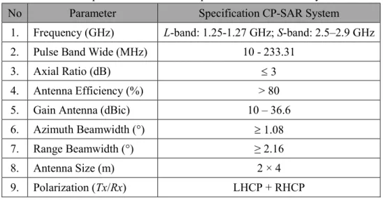
Table 1.1 Specification of antenna parameter for CP-SAR System
No Parameter Specification CP-SAR System
1. Frequency (GHz) L-band: 1.25-1.27 GHz; S-band: 2.5–2.9 GHz
2. Pulse Band Wide (MHz) 10 - 233.31
3. Axial Ratio (dB) 3
4. Antenna Efficiency (%) > 80
5. Gain Antenna (dBic) 10 – 36.6
6. Azimuth Beamwidth (°) 1.08
7. Range Beamwidth (°) ≥ 2.16
8. Antenna Size (m) 2 × 4
9. Polarization (Tx/Rx) LHCP + RHCP
8
Chapter 2
Simple configuration of triangular microstrip array antennas
2.1 Introduction
In this chapter, a simple configuration of triangular microstrip array antennas is discussed, to conduct the selected triangular shape for the better form of array microstrip antennas rather than the other way, such as rectangular, circular, etc. (see Figure 2.1). For the ease discussion, we separate the explanation into five parts specifically (i) Proximity coupled feed using a hole/slot on conducting patch for triangular microstrip array antenna, (ii) Microstrip-line feed using stub for triangular microstrip array antenna, (iii) Coaxial feed for stack-patch triangular microstrip array antenna (Rx) including its fabrication, (iv) Coaxial feed for stack-patch triangular microstrip array antenna (Tx and Rx) including its fabrication, (v) Proximity coupled feed of triangular microstrip array antenna. Moreover, part (i), (ii), (iii), and (iv) are applied for mobile satellite communication, while part (v) is implemented for CP-SAR system, in which the specifications for all of them are listed in Section 2.3. Furthermore, in part (iv), it is a little bit discussed the rectangular shape to distinguish that triangular shape more configurable rather than rectangular shape, because of simultaneity of Tx and Rx in a planar array.
Figure 2.1 Microstrip patch shape [17, 18]
Square Rectangular Dipole Circular Ellipse
Triangle Circular
ring Ring
sector
9
2.2 Feeding
2.2.1 Microstrip line feed
One of the simplest methods of feeding, a microstrip line feed, is shown in Figure 2.2. The feed is located in the same plane as the antenna. Then, the impedance match is realized by changing the amount that the line is inset into the antenna. However, the asymmetry introduced by the feed produces spurious radiation, and it is impossible to optimize the feed circuitry and the antenna simultaneously.
Figure 2.2 Microstrip line feed [17, 18]
2.2.2 Coaxial feed
In Figure 2.3, coaxial feed involves the vertical connection of a coaxial cable conductor through the ground plane to the patch. This method is relatively simple to fabricate and to match.
But, it is more difficult to model and also inherently asymmetrical that can cause spurious radiation because of the presence of vertical currents in the probe (as contrasted to horizontal currents in the patch).
Figure 2.3 Coaxial feed [17, 18]
2.2.3 Proximity coupled feed
From the two feeds described above, the proximity coupled feed shown in Figure 2.4 has the largest bandwidth. It is rather easy to model and has low spurious radiation. However, its
Patch
Coaxial connector Ground plane
Top view Side view
10
fabrication is more difficult. The length of the feeding stub and the width-to-line ratio of the patch can be used to control the match. This structure has the drawback of adding parasitic radiation from the line to the one emitted by the antenna.
Figure 2.4 Proximity coupled feed [17, 18]
2.3 Antenna specifications
2.3.1 Specifications for mobile satellite communication
The specifications and targets of the developed antenna are shown in Table 2.1. ETS-VIII will conduct orbital experiments on mobile satellite communications and high-speed packet communications providing voice/data communications with hand-held terminals in the S-band frequency (2.5025 GHz and 2.6575 GHz for reception and transmission, respectively). The polarization is Left-Handed (LH) circular for both transmission and reception units. As this antenna is assumed to be used in Tokyo and its vicinity, the targeted elevation angle is set to 48°
because it is the elevation angle of the geostationary satellite seen from the center of this city [19, 20].
2.3.2 Specifications for CP-SAR system
In Chapter 1, Table 1.1 shows the specification and the desired target for CP-SAR system, which influence the specification of the L-Band CP-SAR airspace antenna [12]. Each antenna can generate a wave that yields a Circular Polarization (CP). The technique to achieve CP can be easily obtained namely by adequately adjusting the element parameters, determining locus feed, and designing corporate feeding-line [7, 8, 21]. In the simulation of the triangular antenna, the significant variation performances are also affected by the shaping of feeding and their position toward the
Microstrip
line
Patch
11
radiating patches, especially S-parameter, frequency characteristic, input impedance, and radiation pattern.
Table 2.1 Specifications and targets for ETS-VIII applications SPECIFICATIONS
Frequency bands
Transmission (Tx) 2655.5 MHz to 2658.0 MHz Reception (Rx) 2500.5 MHz to
2503.0 MHz Polarization Left-handed circular polarization for both
Tx and Rx OBJECTIVES
Angular ranges Elevation angle (El) 48
o(Tokyo) Azimuth angle (Az) 0
oto 360
oMinimum gain more than 5 dBic
Maximum axial ratio less than 3 dB
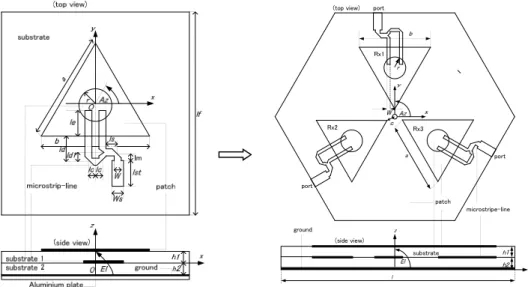
2.4 Proximity coupled feed using a hole/slot on conducting patch for triangular microstrip array antenna
2.4.1 Structure of the antenna
Figure 2.5 depicts the configuration of a single and an array equilateral triangular-patch with a hole, using a conventional substrate (relative permittivity 2.17 and loss tangent 0.0009).
The antenna is fed by proximity feed with microstrip lines whose width W is 3.0 mm for Rx to
obtain a thin configuration. A novel dual feed type with a hole is proposed for the generation of
a compact LHCP using a small equilateral triangular-patch, where one of the microstrip lines
feeds is longer than the other introducing a 90° phase delay. In the same manner, a Right-Handed
Circular Polarization (RHCP) could be realized by swapping the microstrip lines concerning the
y-axis. The proposed feeding technique is designed to obtain an ideal and stable current
distribution on the triangular-patch surface hence improving the previously developed antennas
[22].
12
In this research, the method of moment (MoM) (IE3D Zeland software) is employed to simulate the model with a finite ground plane [15]. Consideration of the effective thickness of the antenna (see Figure 2.5) allowed either the substrate thickness for the microstrip line or feeding line (substrate 2) and triangular patch (substrate 1) is defined with the other implicit (h
1= h
2= 0.8 mm). The length of the microstrip line inserted under the patch l
eis 11 mm, and a quarter-wave transformer is used to obtain a matching impedance of 50 for Rx. The detailed parameters of the microstrip line for Rx are l
s= 5mm, l
d= 11mm, l
d1= 4 mm, l
c= 3 mm, l
m= 2 mm, l
st= 11 mm, r
= 7 mm. The width of the input microstrip line W
sand patch length parameters (for a = b) obtained are 4.90 mm and 46.15 mm, respectively. In the case of the array antenna, the distance between the tip of patch antenna c is 5 mm, and the length of array antenna configuration l is 153.64 mm.
Also, a hole with the dimension of radius r = 7 mm is embedded in the patch which hole center at the null voltage point of the fundamental TM
10mode of the simple triangular microstrip antenna without a hole. It is then expected that the current path or guide wavelength, λ
gof the TM
10mode with a hole is more length than the current path without hole. Thus the frequency operation can be decreased. And by adjusting the radius hole of r, and the length of l
eand l
c, two orthogonal resonant modes can be of equal amplitudes and 90° phase difference and a compact CP operation on the target frequency at 2.5025 GHz can be achieved, with percent decreasing of length patch about by 12.60 % (a = 52.80 mm to a = 46.15 mm) [22-24].
Figure 2.5 Configuration of antenna, single and array for receiver (Rx)
(top view)
port
microstripe-line
substrate patch
ground
(side view) port
port Rx2 Rx3
Rx1
13
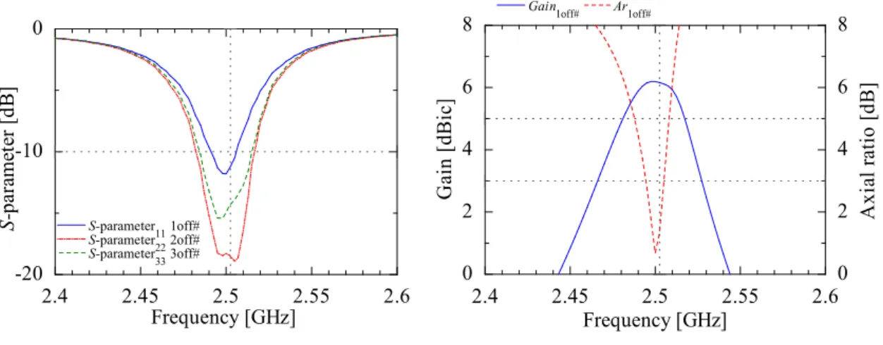
2.4.2 Results analysis
Figure 2.6 represents of the S-parameter, in the case of an array antenna using a hole whereas single element number 1 off, 2 off and 3 off. This figure shows that 2 off is the best compared the others. It is caused by the mutual coupling between fed elements, their phase, and distance that is affected by the finite ground system. Figure 2.7 shows the frequency characteristic.
In the case of single element number 1 off, the gain and axial ratio tend to shift slightly to the below frequency at elevation angle, El = 48.
Figure 2.6 S-parameter Figure 2.7 Frequency characteristic (#1OFF)
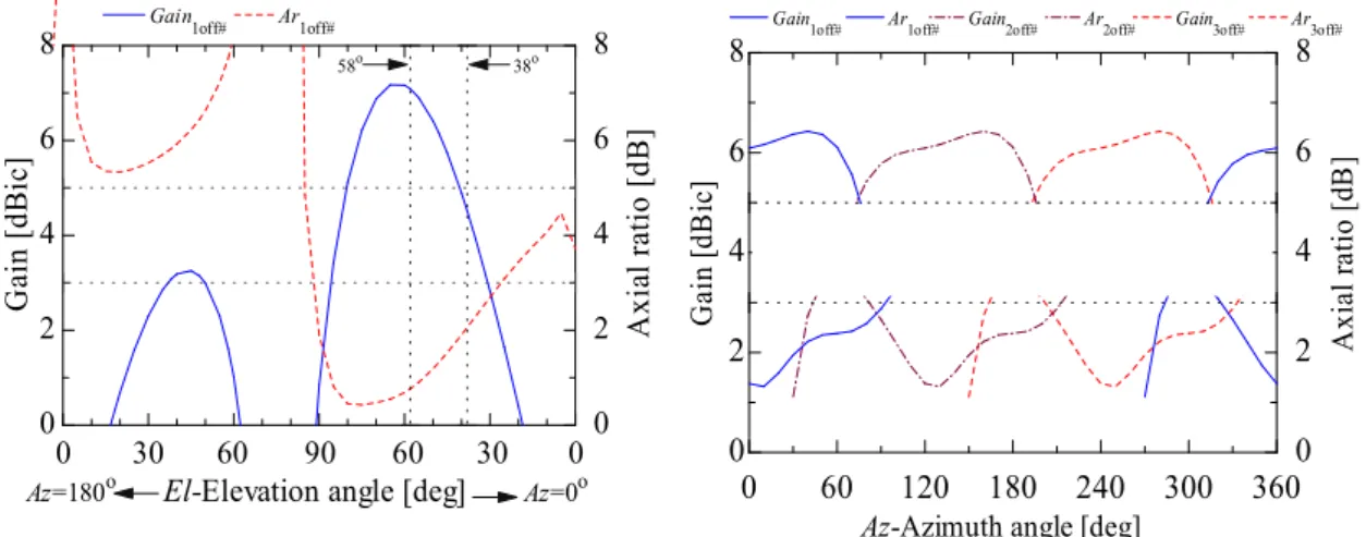
The beam of the antenna is generated by a simple mechanism that consists in switching OFF one of the radiating element of reception shown in Figure 2.5. By considering the mutual coupling between fed elements, their phase, and distance, the beam direction can be varied. Hence, the two feed elements theoretically will generate a beam shift of -90° in the conical-cut direction from the element which is switched OFF, in the case the antenna configuration shown in Figure 2.5. For example, when element #1 is switched OFF, the beam is directed towards the azimuth angle Az = 0° [19].
Figure 2.8 describes the radiation characteristics in the elevation-cut plane angle when element #1 is switched OFF. It is assumed that from northern to southern Japan the elevation angle is 38 to 58 towards the satellite position. According to this figure, the axial ratio satisfies the targets although the gain at the lowest target elevation angle is less than 5 dBic.
Figure 2.9 represents the radiation characteristics in the conical-cut direction. This figure shows that the peak gain and the axial ratio is around 6.82 dBic and 0.66 dB respectively in the
2.4 2.45 2.5 2.55 2.6
-20 -10 0
S-parameter11 1off#
S-parameter22 2off#
S-parameter33 3off#
Frequency [GHz]
S- pa ra m et er [ dB ]
2.4 2.45 2.5 2.55 2.6
0 2 4 6 8
0 2 4 6 8
G ai n [d B ic ] A xi al r at io [ dB ]
Frequency [GHz]
Gain1off# Ar1off#
14
technical beam direction. The gain is satisfied the target above 5 dBic in the 120 coverage for each beam. Also, the axial ratio satisfies less than 3 dB.
Figure 2.8 Elevation-cut plane, Figure 2.9 Conical-cut plane, f = 2.5025 GHz El = 48° f = 2.5025 GHz
2.5 Microstrip line feed using stub for triangular microstrip array antenna
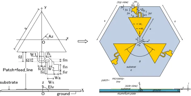
2.5.1 Configuration of antenna
Figure 2.10 illustrates the configuration of the single patch equilateral triangular antenna for an array antenna. The antenna parameters are shown in Table 2.2. The configuration of array antenna consists of three patches with the same parameter size which is rotated 120° each other.
There are three types of parameter size of single for array antenna, namely: without the use of stub with fst = 16 mm and Wa = 0 mm, the use of stub with fst = 14 mm and Wa = 3 mm, and the last ones is the use of stub with fst = 14 mm and Wa = 5 mm. Also, the distance of the tip of the triangle to the central point, lo = 10 mm, the length of hexagonal ground g = 93.07 mm, and the angle between two adjacent patches seen from the central point, θ = 120°. The array antenna is also made from a conventional substrate (ε
r= 2.17 and δ = 0.0009) with the substrate thickness, h
= 1.6 mm. The element patch of this antenna is supplied by microstrip line feed where the width Ws = 7.0 mm for receiver antenna, Rx. Singly-fed forked can generate two waves with different phase 90
0to obtain Left-Hand Circular Polarization (LHCP). In the same manner, the circular polarization wave to the right (RHCP) can be realized by exchanging the microstrip line on the y- axis [25].
0 2 4 6 8
0 2 4 6 8
0 30 60 90 60 30 0
G ai n [d B ic ] A xi al r at io [ dB ]
El-Elevation angle [deg]
Gain1off# Ar1off#
58o 38o
Az=0
oAz=180
o0 0 60 120 180 240 300 360
2 4 6 8
0 2 4 6 8
Gain3off# Ar3off#
Gain2off# Ar2off#
Gain1off# Ar1off#
G ai n [d B ic ] A xi al r at io [ dB ]
Az-Azimuth angle [deg]
15
Figure 2.10 Antenna configuration, single and array for receiver (Rx)
The Method of Moments (MoM) has been chosen for this numerical analysis to make the fast calculation. The software used was Ensemble
TMversion 8 from Ansoft [14]. According to the software characteristics, the dielectric substrate and the ground plane are considered to be infinite.
Table 2.2 Antenna parameters [25]
Parameter Value of Model-1 (mm)
Value of Model-2 (mm)
Value of Model-3 (mm)
a 52.64 52.64 52.64
fd 11 11 11
fd1 3.5 3.5 3.5
fc 3.5 3.5 3.5
fs 5 5 5
fm 3.5 3.5 3.5
fsr 0 4 3
fss 0 7 7
fst 16 14 14
W
12 2 2
W
23 3 3
Wa 0 3 5
Ws 7 7 7
16
2.5.2 Results and discussion
Figure 2.11 to Figure 2.12 show the simulation results of the antenna array, such as S- parameter and frequency characteristics. Figure 2.13 and Figure 2.14 are specific to the performance of the antenna array, namely the vertical and the horizontal radiation patterns.
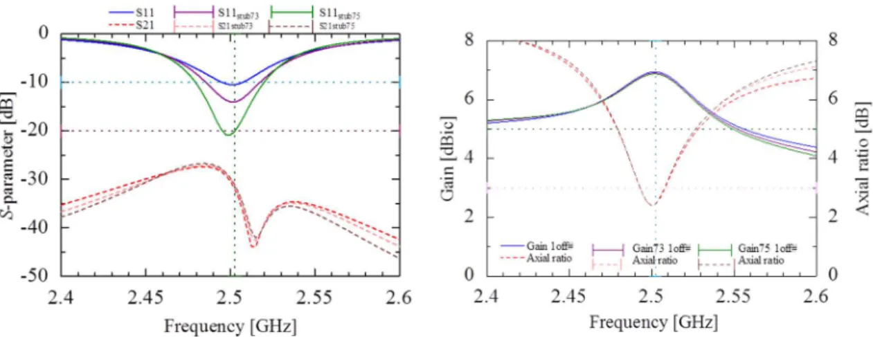
Figure 2.11 shows the relationship between the S-parameters and frequencies for simulation of receiver antenna (Rx). In this figure, it can be seen that the S-parameter (S
11) of the three types of the antenna (without stub-fed, stub-fed
73and stub-fed
75) at the frequency target 2.5025 GHz about -11 dB, -15 dB, and -20 dB, respectively. Then, the S-parameters (S
21) of the three types of antenna are almost the same, roughly -33 dB.
Figure 2.12 shows the value of the gain and axial ratio (Ar) for the three types of simulation well-fed antenna without stub-fed and with stub-fed in different sizes at the frequency target 2.5025 GHz. The value of each gain almost the same, around 6.93 dBic and also this case occur for each axial ratio, roughly 2.43 dB. Also, the gain-bandwidth-5dBic of the three types of the antenna is also almost the same, around 2.59%. The 3-dB axial ratio bandwidth for the three types of the antenna is approximately 0.7%.
Figure 2.11 S-parameter, S
11and S
21Figure 2.12 Frequency characteristic
Figure 2.13 shows the relationship between the characteristics of the radiation (gain-axial
ratio) in the part of Az = 0° and elevation angle when the one of three patches antenna is switched
OFF, and the others are switched ON. The results indicate that from the northern tip to the southern
tip of Japan elevation angle of 38° to 58° relative to the satellite position (above the equator) for
the three types of antenna mentioned above yield the desired target.
17
Figure 2.13 Elevation-cut plane, Figure 2.14 Conical-cut plane, f = 2.5025 GHz El = 48° f = 2.5025 GHz
Figure 2.14 describes the characteristic of conical pieces radiation in the El = 48° area. In this figure is seen that the peak of the gain and axial ratio for the three types of antenna are almost the same, around 7.56 dBic and 0.13 dB, respectively. Also, the values of the gain and axial ratio beamwidth meet the target for beam coverage of 120°.
2.6 Coaxial feed for stack-patch triangular microstrip array antenna (Rx) including its fabrication
2.6.1 Configuration of antenna
Figures 2.15 (a) and (b) illustrate the array antenna configuration aimed at mobile satellite communications (
r= 2.17, loss tangent 0.0009). The antenna is composed of three pentagonal patch antennas fed directly from the ground beneath the construction to radiating patch, instead of using three coaxial/probe feeds. At the top of the construction, it lies three triangular patches as parasitic elements. The dimension of the construction is 160 mm and 6.4 mm in diameter and height, respectively. Three single patch antennas are arranged in 120° difference to one another in the azimuth rotation to form the array antenna structure. The distance between two elements by viewing from the apex of the patch antenna is about 0.5λ to generate a beam directed as desired.
The radiation characteristics of such kind of array configuration were reported in [26], where the array antenna can produce three beams in different azimuth direction (Az = 0°, 120°, and 240°).
Moreover, the distance between the tip of the antenna element and the center point of array
composition is set in different length for radiating and parasitic element. By considering the axial
18
ratio performance, their distance is set at 8.7 mm and 9.7 mm for fed and a parasitic elements, respectively. The proposed array antenna is applied for reception purpose. With this composition, a dual-band operation antenna with the reception and transmission antennas arranged in one dimension can be achieved. Besides, the array antenna is mounted on a stacked-parasitic patch to enhance the gain and bandwidth. Moreover, when this way is constructed, the loss of the switching circuit from beneath the array antenna may be compensated.
For a patch antenna, in case the radiating element is loaded with a parasitic element on its top, it is possible to obtain a higher gain and a wider bandwidth by using the multiple resonances generated by the radiating element itself and the parasitic element [26-30]. Figure 2.15 (a) shows the configuration of the triangular patch array antenna with the parasitic element and Figure 2.15 (b) shows the fabricated antenna. The circularly polarized radiation is obtained merely by the use of large truncation corner on the driven patch. This truncation corner can control the two orthogonal modes (mode #1 and mode #2 in Figure 2.16) on the patch [31]. The area of the truncation corner is wider than a single layer because the parasitic patch expands the Q of each mode; i.e., the resonant frequency of each mode can be widely separated. Accompanied with the feeding location and to match the 50 Ω matching input impedance, a 4 mm-air gap is inserted in the space between the radiating and parasitic elements. Moreover, the antenna can be fitted to the required frequency by varying a feed location, air gap thickness, and antenna dimension. With this consideration, the antenna resonates at 2.5025 GHz as a target frequency for reception antenna (Rx) in mobile satellite applications. Besides, by setting the isosceles length of the parasitic element to be shorter with a ratio of 0.95 to other sides, a good axial ratio CP operation can be obtained [32].
In this configuration, the fabricated antenna is low profile, small, and lightweight to be
mounted on the car-rooftop, and the generated-antenna beam is always directed to the east
longitude of 146° where the mobile satellite is orbited.
19
(a) Calculation array antenna (b) Fabricated array antenna Figure 2.15 Stack-Patch array antenna configuration of Rx
Figure 2.16 The two orthogonal modes with truncation corners
2.6.2 Performance of results analysis
Figures 2.17 to 2.21 illustrate the results from both calculation and measurement regarding S-parameter, axial ratio characteristic, and radiation pattern. The difference between the calculation and measurement that appears in the results is because a finite ground is used in the measurement while it is infinite in the calculations. Figure 2.17 demonstrates that the measured S
11tends to meet the calculated value. The impedance bandwidth (S
11< -10 dB) is about 6.93%.
The isolation is more than 25 dB which is above the target isolation of 20 dB.
c h
a c l
b Patch
Mode#1
Mode#2 Feeding
point
Truncation corner
10.8 mm
1.6 mm Ground
Dielectric constant
= 2.17 z 4.0 mm
r El 0.8 mm
Parasitic element Fed element
Fed element 53.6 mm 8.7 mm
y
#3
#2 #1
#3
#2 #1
#3
#2 #1 Az x
#3
#1
#2
Parasitic element
9.7 mm x y Az 9.7 mm x
y Az 9.7 mm x
y Az
53.24 mm
53.4 mm 9.7 mm x y Az
Top view
Side view 6.76 mm
39.8 mm
10.8 mm
1.6 mm Ground
Dielectric constant
= 2.17 z 4.0 mm
r El 0.8 mm
Parasitic element Fed element
Fed element 53.6 mm 8.7 mm
y
#3
#2 #1
#3
#2 #1
#3
#2 #1 Az x
#3
#1
#2
Parasitic element
9.7 mm x y Az 9.7 mm x
y Az 9.7 mm x
y Az
53.24 mm
53.4 mm 9.7 mm x y Az
Top view
Side view 6.76 mm
39.8 mm
20
Figure 2.18 illustrates that the measured result of axial ratio increases to 1.0 dB at frequency 2.5025 GHz and El = 48° or θ = 42°. Moreover, the 3 dB axial ratio bandwidth gets about 1.7%.
The measurement result is worse than the calculated result due to the variation in the measurement during the fabrication process. In order to match between measurement result of fabricated antenna and the calculation result, the antenna was optimized until the measurement result suits the target for mobile satellite applications. Here, the result satisfies the target although a little bit decreased.
The axial ratio satisfies the target less than 3 dB, and the gain is more than 5 dBic at elevation angle El = 38° – 58° or θ = 32° – 52° as shown in Figure 2.19 at f = 2.48 GHz for calculation and f = 2.5025 GHz for measurement. This condition is achieved by having one of three ports switched OFF, and the others biased ON. This mechanism produces a beam that could be directed at the desired target.
The beam of the antenna is generated by a simple ON-OFF mechanism that consists of one out of three radiating elements being turned off. For that reason, there is three OFF state beam switching mechanisms: #1 OFF, #2 OFF, and #3 OFF. By considering the mutual coupling between fed elements, their phases, and distances, the beam direction can be varied. Furthermore, the two feed elements theoretically will generate a beam shift of -90° in the conical-cut direction from the element which is switched OFF. For example, when element #1 located at Az = 30° is switched OFF, the beam is directed towards the azimuth angle Az = -60° or 300° as shown in Figure 2.15 (a) [32].
Figure 2.17 S-parameter, S
11Figure 2.18 Axial ratio characteristic
2.40 2.45 2.50 2.55 2.60 2.65 0
2 4 6 8 10
Frequency [GHz]
A r - a xi al r at io [ dB ]
Calculation Measurement
2.40 2.45 2.50 2.55 2.60 2.65 -40
-30 -20 -10 0
Frequency [GHz]
S pa ra m et er [ dB ]
Calculation Measurement
S
Isolation
11
21
Figure 2.19 Elevation-cut plane
The measured results of gain and axial ratio characteristics of the beam switching in the azimuth plane are shown in Figure 2.20 and Figure 2.21 at f = 2.48 GHz for calculation and f = 2.5025 GHz for measurement. The tendency of the measurement results is the same as the calculated ones. The measured results show that at the center beam, the gain of each beam is averaged about 0.2 – 0.5 dB less than that of the calculation results. The axial ratio increases for each OFF condition, but the 3-dB axial ratio coverage of the measured result can cover 360° in the conical-cut plane at El = 48°. Moreover, the beam is possibly switched at a minimum gain of 6.3 dBic. Also, although the axial ratio is shifted from the switched point, to cover 360° conical plane the minimum axial ratio below 3 dB is possible to obtain. This elevation is applied in Kanto area.
Figure 2.20 Conical-cut plane, gain vs Az Figure 2.21 Conical-cut plane, Ar vs Az 0
2 4 6 8 10
0 2 4 6 8 10
90 60 30 0
60 30 0
Az = 180 ° Az = 0 °
El - Elevation angle [deg]
G - ga in [ dB ic ] A R - ax ia l r at io [ dB ]
Calculation Measurement
0 90 180 270 360
0 2 4 6 8 10
Az - Azimuth angle [deg]
G - g ai n [d B ic ] 1OFF 2OFF 3OFF 1OFF Calculation Measurement
Elv 48o
0 90 180 270 360
0 2 4 6 8 10
3OFF 1OFF 2OFF
Az - Azimuth angle [deg]
A R - a xi al r at io [ dB i]
Calculation Measurement
Elv 48o
22
2.7 Coaxial feed for stack-patch triangular microstrip array antenna (Tx and Rx) including its fabrication
2.7.1 Configuration of antenna
The antenna structure of six-element array antenna is depicted in Figure 2.22 (a) (
r= 2.17, loss tangent 0.0009). The array antenna instead of three pentagonal patch antennas as radiating for its reception and transmission which each element directly fed by three coaxial/probe feed are located on the beneath of the construction. In the top of the construction is laid three isosceles triangular patches as parasitic elements. The proper feeding location on the radiating patch is chosen for matching with 50 Ω input feed. For more strength of matched with 50 Ω, air-gap is inserted at the area between the fed elements and the parasitic elements. Moreover, the function of feeding is to trigger the dominant mode and higher mode, to make circularly polarized, and to reduce the coupling with element one half [33].
While the other air-gap function is to widen bandwidth and to increase the gain. Similar
with the air-gap function, for more stability of it, the parasitic element is operated for not only
that purpose, but also to make smooth circular polarized and to adjust coupling with the element
beside it. In a matter of coupling, the distance between the apex of both transmission and reception
element to the center point of array are set 9.7 mm and 19.7 mm, respectively. It is meant to
reduce isolation with each closer patch and thus to get sufficient gain for obtaining the minimum
requirement 5 dBic. Usually, for decreasing coupling to patch element closer each other, the
needed distance between center of patch element (in this case 1/3 h, where h is a height of patch
antenna) to the other closer patch element (d) is based on the formula 0.5 λ < d < λ, where λ is the
wavelength of used [34]. Furthermore, based on investigate in calculation on Figure 2.22 (a) the
both of coupling and current distribution are increased parallel with counter-clockwise moved,
for example, coupling patch R1T1 > coupling patch R1T3 (seen Figure 2.25). In the otherwise
manner coupling and current distribution become decreased. The construction of this antenna
makes possible for exciting the two near-degenerate orthogonal modes of equal amplitudes and
90° dimension phase difference for LHCP operation [35]. The dimension of the construction is
160 mm and 6.4 mm in diameter and height, respectively. The fabricated antenna is pictured in
Figure 2.22 (b) that show triangular array antenna more configurable (Tx and Rx in one planar
substrate) rather than rectangular array antenna (Tx and Rx in two planar substrates separately,
see Figure 2.23).
23
(a) Calculation array antenna (b) Fabricated array antenna Figure 2.22 The construction of 6-elements array antenna for Tx and Rx
Figure 2.23 The construction of rectangular array antenna, separately Tx and Rx [26]
To help conduct the study, Ensemble version 8.0 is used to design and develop the model
for those antennas. The use of such software provides some advantages for industry and
researchers when developing new and unproven telecommunication technologies such as the
ability of to conduct a preliminary study of the new antenna design (as an example) without
having to build a hardware prototype.
24
2.7.2 Results and discussion
Figure 2.24 to Figure 2.28 notices the results for both simulation and measurement, in the case of S-parameter, axial ratio characteristic, elevation-cut plane, and conical-cut plane. The difference between the calculation and measurement present in the results since a finite ground is used in the measurement and infinite ground in simulations.
Figure 2.24 shows that the measured S
11both of Tx and Rx tends to meet the calculation ones. Moreover, the bandwidth below -10 dB of Rx in calculation and measurement results are 7.79% and 8.39%, while the bandwidth results of Tx are 6.21% and 6.02%, respectively. At the frequency target in Rx = 2.5025 GHz, the value of S
11in calculation and measurement are -10.56 dB and -12.15 dB rather than Tx = 2.6575 GHz about -13.13 dB and -12.86 dB, respectively. The isolation between elements located close to each other is more than 10 dB which is below the target isolation 20 dB. But the tendency of calculation and measurement results are met each other (see Figure 2.25).
Figure 2.24 S-parameter, S
11Figure 2.25 S-parameter, S
21Figure 2.26 illustrates that the measured results of axial ratio both Tx and Rx are a shift to the higher frequency of about 2.79% and 1.32%, respectively. Moreover, the 3-dB axial ratio bandwidth gets both of Tx and Rx measured about 1.89% and 1.22% rather than calculated results about 1.99% and 1.69%, respectively. Moreover, the calculation results of gain versus frequency both Tx and Rx at the frequency targets 2.48 GHz and 2.63 GHz are 5.69 dBic and 6.9 dBic, respectively (see Figure 2.27).
2.4 2.45 2.5 2.55 2.6 2.65 2.7 2.75 2.8 -40
-30 -20 -10 0
S-R1T1
simS-R1T3
simS- pa ra m et er [ dB ]
Frequency [GHz]
S-R1T1
measS-R1T3
measIsolation
25
Figure 2.26 Axial ratio characteristic Figure 2.27 Frequency characteristic
The axial ratio satisfies the target less than 3 dB and the gain more than 5 dBic at elevation angle El = 38 - 58 or θ = 32° - 52° both of Tx and Rx in calculation and measurement result as shown in Figure 2.28 and Figure 2.29. The resonant frequencies of calculation are f = 2.63 GHz for Tx and f = 2.48 GHz for Rx. Moreover, the resonant frequencies of measurement are f = 2.6575 GHz for Tx and f = 2.5025 GHz for Rx. This condition achieved by one of three ports is switched OFF, and the others bias ON. These mechanisms make a beam that could be directed suit with the desired target.
The beam of the antenna is generated by a simple ON-OFF mechanism that consists in one out of three radiating elements to be turned off. For that reason, there are three OFF states beam switching mechanism, i.e., #1 OFF, #2 OFF, and #3 OFF. By considering the mutual coupling between fed elements, their phases, and distances, the beam direction can be varied. Furthermore, the two fed elements theoretically will generate a beam shift of -90° in the conical-cut direction from the element which is switched OFF. For example, when element Rx #1 located at Az = 90°
is switched OFF, the beam is directed towards the azimuth angle Az = 0° (see Figure 2.22).
The measured results of gain and axial ratio characteristics of the beam switching in the azimuth/conical plane are shown in Figure 2.30 (f = 2.63 GHz in calculation and f = 2.6575 GHz in measurement, Tx) and Figure 2.31 (f = 2.48 GHz in calculation and f = 2.5025 GHz in measurement, Rx). The tendency of the measurement results is the same as the calculation ones.
The measured results of Rx show that at the center beam, the gain of each beam is matched with the calculation results while in Tx at the center beam the gain is averaged down in 0.1 – 0.3 dB rather than the calculation results. The axial ratio increases for each OFF condition, but the 3-dB
2.4 2.45 2.5 2.55 2.6 2.65 2.7 2.75 2.8 0
2 4 6 8 10
0 2 4 6 8 10
G ai n [d B ic ] A xi al r at io [ dB ]
Frequency [GHz]
Gain
RxAr
RxGain
TxAr
Tx26
axial ratio coverage of the measured result can cover 360° in the conical-cut plane at El = 48°, in case of Rx. It difference for Tx that the measured result can cover the whole of azimuth 360° if only the axial ratio exists at around 4 dB. Moreover, the beam is possibly switched at minimum gain about 6 dBic both of Rx and Tx, and although the axial ratio is shifted from the switched point, to cover 360° conical-plane, the minimum axial ratio below 3 dB is possibly obtained, especially for Rx. This elevation is applied at Kanto area.
Figure 2.28 Elevation-cut plane, Tx Figure 2.29 Elevation-cut plane, Rx
Figure 2.30 Conical-cut plane, Tx Figure 2.31 Conical-cut plane, Rx 0
2 4 6 8 10
0 2 4 6 8 10
0 30 60 90 60 30 0
G - ga in [ dB ic ] A R - ax ia l r at io [ dB ]
El - Elevation angle [deg] Az = 60°
Az = 240 °
Calculation Measurement
0 60 120 180 240 300 360
0 2 4 6 8 10
0 2 4 6 8 10
G ai n [d B ic ] A xi al r at io [ dB ]
Az-Azimuth angle [deg]
Elv 48o
1off# 2off# 3off#
Calculation Measurement Rx
0 60 120 180 240 300 360
0 2 4 6 8 10
0 2 4 6 8 10
G ai n [d B ic ] A xi al r at io [ dB ]
Az-Azimuth angle [deg]
Elv 48o
![Figure 1.1 Miniature of a CP-SAR triangular array antenna consisting of microstrip elements [7]](https://thumb-ap.123doks.com/thumbv2/123deta/5639832.2003235/14.892.238.649.377.543/figure-miniature-triangular-array-antenna-consisting-microstrip-elements.webp)
![Figure 2.3 Coaxial feed [17, 18]](https://thumb-ap.123doks.com/thumbv2/123deta/5639832.2003235/20.892.159.740.734.949/figure-coaxial-feed.webp)
![Figure 2.4 Proximity coupled feed [17, 18]](https://thumb-ap.123doks.com/thumbv2/123deta/5639832.2003235/21.892.201.692.273.473/figure-proximity-coupled-feed.webp)