AN APPROACH TO CALIBRATING A GENERAL EQUILIBRIUM MODEL INCORPORATING AN INPUT-OUTPUT ACCOUNTING MATRIX

(1)

AN APPROACH TO CALIBRATING A GENERAL EQUILIBRIUM MODEL INCORPORATING AN INPUT-OUTPUT ACCOUNTING MATRIX

HIDETAKA KAWANO*

1. INTRODUCTION

An applied general equilibrium model is a powerful analytical framework with which to examine the policy effects on the entire network of an economy. One of the important developments since Scarf (1967) has been the use of observed data such as an input-output accounting matrix. One of the important steps for the empirical characterization of a model is so-called "calibration." Calibration is defined as "the requirement that the entire model specification be capable of generating a base-year equilibrium observation as a model solution" (Shoven and Whalley, 1992: 103). In this paper, I demonstrate a simple way to calibrate parameters so as to incorporate actual input-output data into a general equilibrium model. The model structure is a two-sector and two-factor closed economy with two intermediate goods flows in production activities. Both preference and technology are assumed Cobb-Douglas.

For base data, I group the 1995 Aomori Prefecture I3-sector input-output data set (Sep., 1999) into two sectors. One is the agricultural sector, defined as industry O. The other is a highly aggregated non-agricultural sector, defined as industry 1. The final consumption data includes net export in value terms.

The organizing solution procedure for coding the model follows Shoven and Whalley (1992: 43-4) by reducing the dimensionality of the solution space to the number of factors of production in this general equilibrium structure. The solution algorithm used for calibration is a fixed-point algorithm originally developed by Kimbell and Harrison (1986) and modified by Kawano (2003).

For the replication check, the calibrated parameters were capable of generating a base- year equilibrium observation as a model solution. This data can therefore be considered an appropriate benchmark for various comparative static experiments. Calibration results show that the unit-price convention is kept in goods markets as well as factor markets.

(2)

This experiment was conducted using Intel's 333MHz Pentium II processor and was programmed in C-language. The verified reliability of the simulation results resulted in double precision (1.0e-16). The converged equilibrium values were obtained through 44 iterations over the entire model.

The main strength of this calibration approach is that it is easily extended to deal with larger multisector models. A possible weakness is that the number of iterations for the convergence of equilibrium values is relatively increased as the model dimensions increase.

In section 2, the general structure of the model is specified. In section 3, the calibration procedure is described. The conclusion follows in section 4. All notations are defined as they appear for the first time in the text, and, in Appendix A, is a list of variable definitions.

2. THE GENERAL STRUCTURE OF THE MODEL

2.1. The main features of the model

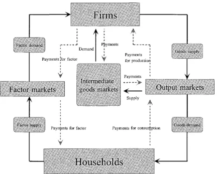
The supply side of a theoretical general equilibrium model is made more empirically plausible by incorporating a Leontief type input-output accounting data. An important step in building an empirical model is to incorporate flow of intermediate goods into the model structure. The flow of intermediate goods among different sectors is built into the model as part of production activity in the economy. Figure 1 shows flows of intermediate goods in the model.

Figure 1 The flow diagram of a closed economy with intermediate goods flows

r ^P~yments

Demand ~

Payments ror ^factor .~ ^Paymentsfor productio~ ^,

,

Payrrtents for factor

~ ~'~~~~~~~

.

Supply

,

Payments for consu~ption

, ,

(3)

The entire model has two sectors, shown by subscript i E I = {O, I}, and two final consumption commodities ^{Xi d.} The use of intermediate goods in production activities shows that total output Qi Ê¹in sector i will go partly to meet final household consumption demand Xi E 1 , and also intermediate input demand qij for production of goods j EJ = {0,1}. The production activities of firms include intermediate goods Q_{i d} supplied through output markets. The usual primary factors of production are capital Ki Ê¹and labor Li Ê^1· In the Leontief system, intermediate inputs are required as a fixed proportion of the total output Q_iÊ1. All relevant input-output information is summarized in Table 1. The input-output coefficients aij are defined as:

where

= qii

aij - Q

j

, ViE!, jEj. (1)

aij := input-output coefficient for commodity i used as an intermediate good to produce one unit of commodity j,

qij := amount of commodity i used as an intermediate input for production of commodity j,

Qj := output in industry j.

Table 1. Two-sector economy with intermediate goods flows

Industry 0 Industry 1

Inputs to industry 0 qoo = aooQo qlO = _aloQo

2.2. The demand side of the model

Input to industry 1 qOl = aolQl qll = allQl

Final

consumption

Xo Xl

Total output

Q_o Q_l

The level of disposable income for a representative consumer is determined by factor endowments and factor prices. The disposable income is:

y= wL+rK,

where

w := wage rate, r := rental rate,

L := labor endowment, K := capital endowment.

(2)

(4)

I assume Cobb-Douglas utility function as a representation of consumer preference. The function is:

(3)

The final demand for commodities Xi ^EI is derived by the utility maximization for a representative consumer.

X· = eⁱ^Y ^ViE^I.

t Pi'

where

8_i^E^I:= share parameter in utility function,

Pi := price of commodity .

2.3. The production side of the model

The production function with intermediate inputs is modeled as:

Q -^{j -} ^mIn.

(!liL

^,

VA)

^{j '}

aij

ViEI,jEj.

where

V Aj ^{E ]} := value-added component of production function j E ].

(4)

(5)

The value-added component V Aj EJ of production function j E j is modeled as Cobb- Douglas which allows the substitution possibility between primary factors: capital K_j and labor Lj • The value-added component VAj is specified as:

where

ai ^EI := factor share parameter in value-added component of production function,

<D i E I := shift parameter in value-added component of production function, Ki ÊÎ:= capital employed in sector i ÊI,

Li ^E^I:= labor employed in sector i E 1.

(6)

(5)

The conditional factor demand functions are derived as if there are no intermediate goods in the model, since a fixed proportion of the total output Q_idoes not affect the first order conditions of the producers' cost minimization.

1) The per unit capital demand function is:

k

i

=

_1_(

^aⁱ )1-ai(~)I-ai

,

^{ViE J.}

<Di 1 -a_i r ⁽⁷⁾

2) The per unit labor demand function is:

(8)

2.4. Zero profit conditions

Perfectly competitive behavior in producers will imply zero profit conditions. Zero profit conditions for the two producers with intermediate goods are modeled as:

F or the producer in sector i E J,

I

Pi = Lajj)j+rki+wli, ^ViEJ.

j=o

where

k_i:= capital employed for per unit production of commodity i E J,

li := labor employed for per unit production of commodity i E 1.

Rewrite equations (9) in matrix as:

where

A

0] ,

^p ⁼ ^{[Po], w}⁼ [rko+wlo].

1 PI rki +wl i

Solve for P .

(9)

(10)

(11)

(6)

2.5. The market clearing conditions

The total output Q_i^EI of commodity in sector i E I is met by the total intermediate input

1

demand L ^q^ijand final consumption demand Xi ^EI j=O

1

Q i = L ^q^ij+ Xi , 'v' i ^EI.

j=O

By equation (1), qij = aijQj' Rewrite equation (12) as:

1

Qi = L aijQj+ Xi' 'v'i E I.

j=O

Further rewrite equation (13) in matrix as:

(I-A)Q ⁼ X,

where

Solve for Q.

(12)

(13)

(14)

(15)

Appendix B shows the entire structure of the general equilibrium model incorporating intermediate goods in production.

3. CALIBRATION PROCEDURE

Here, I use "calibration" to mean building a general equilibrium model to be consistent with an actual data set. In other words, choose the model parameters to replicate the real data at hand. I present a computational procedure to calibrate parameters so as to incorporate actual input-output data into a general equilibrium model.

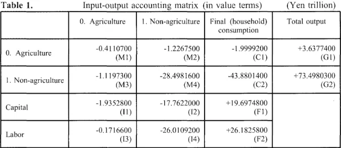
Step 1: group the 1995 Aomori Prefecture 13-sector input-output data set into two sectors.

One is the agricultural sector, defined as industry O. The other is a highly aggregated non- agricultural sector, defined as industry 1. The final consumption data includes net export in value terms. The aggregated input-output accounting matrix shown in Table 1 is constructed

(7)

for the calibration of the model.

Table 1. Input-output accounting matrix (in value terms) (Yen trillion) O. Agriculture 1. Non-agriculture Final (household) Total output

consumption

O. Agriculture -0.4110700 -l.2267500 -1.9999200 +3.6377400

(Ml) (M2) (Cl) (Gl)

1. Non-agriculture -l.1197300 -28.4981600 -43.8801400 + 73.4980300

(M3) (M4) (C2) (G2)

Capital -l.9352800 -17.7622000 + 19.6974800

(11 ) (12) (Fl)

Labor -0.17l6600 -26.0109200 +26.1825800

(I3) (I4) (F2)

Step 2: Read information from the input-output data file into the calibration program. The program uses the data to calibrate parameters. The calibrated parameters are: 1) consumption-share parameters ^f)iÊ^J, 2) factor-share parameters a_iÊ^J, intermediate-input coefficients âid,fE]' and 3) shift parameters in production <Did' These parameters are computed in double precision and presented at the beginning of the output file in Appendix C. The key calibration equations are: a_o= 11/ (11 + 13), a_l = 12/ (12+ 14) , f)o = C1/(C1+C2), a_oo = M1/G1, _{a OI} = M2/G2, _{a lO}= M3/G1, all = M4/G2,

¢o = G1/(I1aoI31-ao) , and ¢l = G2/(I2alI41-al). Note that commodity prices are converged to unity, as shown in lines (3) and (4). Factor prices are converged to unity, which are shown in lines (8) and (9). Also note that the calibrated parameters are all general-equilibrium consistent. Marginal rate of substitution (MRS) equals the relative price of good 0 (PO/PI) in lines (1) and (2). Marginal rate of technical substitutions (MRTS_{o and}MRTS_{I )} equal the relative price of labor (w/ r) in lines (5) through (7).

Marginal rate of transformation ( MR T ) equals the relative price of good 0 (P 0/ PI) in lines (10) and (11).

Step 3: Generate a micro-consistent data set. The data is summarized in the social accounting matrix form shown in Table 2. Its zero-sum row shows that all goods and factor markets are cleared. Its zero-sum column shows that income equals expenditure in each sector. The generated data set shows micro-consistent financial flows in all sectors of the economy. In other words, the data is consistent with the underlying general equilibrium structure of the model.

(8)

Table 2. Social Accounting Matrix (in value terms) (Yen trillion)

o. Agriculture l. Non-agriculture Final (household) Row sum consumption

o. Agriculture +3.2266700 -l.2267500 -1.9999200 0.0000000

l. Non-agriculture -l.1197300 +44.9998700 -43.8801400 0.0000000

Capital -1.9352800 -17.7622000 +19.6974800 0.0000000

Labor -0.1716600 -26.0109200 +26.1825800 0.0000000

Column sum 0.0000000 0.0000000 0.0000000

Note: Income is shown as a positive entry, expenditures shown as a negative entry.

Step 4: Conduct the replication check to see if the calibrated solutions in the model is error- free in building and coding the model. The generated data is exactly identical to both the original input-output accounting matrix data in Table 1 and the social accounting matrix data in Table 2. I list calibrated parameters and the variables of interest in Table 3. The replication check has passed, so that the data is considered as an appropriate benchmark for comparative static experiments. The complete output file is presented in Appendix C.

Table 3. Results of the calibration

Calibrated parameters and the related variables of

Calibrated values and some related values interest

eo 0.043590178391223

I-eo 0.956409821608777

a o 0.918526393727396

I-a o 0.081473606272604

a) 0.405778706201431

I-a) 0.594221293798569

aoo 0.113001478940221

aO) 0.016690923552645

alO 0.307809244201070

all 0.387740460526629

<Do 2.289834882539788

<D) 3.298685130085004

(9)

K 19.69748000000000 (Imposed)

L 26.182580000000000 (Tmposed)

Note: The shaded areas show that the conditions for general equilibrium models are satisfied in both methods.

4. CONCLUSION

This paper shows an approach to incorporating an input-output accounting matrix to calibrate a general equilibrium model. The model makes use of a simple Cobb-Douglas technology and preference. For this calibration, I grouped the 1995 Aomori Prefecture 13- sector input-output data into two sectors. One is the agricultural sector defined as industry O. The other is a highly aggregated non-agricultural sector defined as industry 1. The final consumption data includes net export in value terms. The aggregated input-output accounting matrix is shown in Table 1. The 9 calibrated parameters are; eo, ^a^{0 '}^{aI' a}^{00 ,}

a 01 , a 10' a l l ' <D ^0'<D ^{l '}For the replication check, the calibrated parameters produced both the exactly identical input-output accounting matrix in Table 1 and the related social accounting matrix in Table 2. This data can therefore be considered as an appropriate benchmark for comparative static experiments. The main strengths of the calibration approach is that it is relatively easily extended to incorporate multisector models. A possible weakness is that the number of iterations for the convergence of equilibrium values is relatively increased.

Received: January 13,2004, Accepted: January 15, 2004

(10)

References

Aomori Prefecture input-output table (1999) Aomori-ken Kikaku-bu toukei-ka, Aomori.

Kawano, H (2003) "A Simultaneous Multi-Factor Price Revision for Solving a Numerical General Equilibrium Model," Aomori Public Col/ege Journal of Management & Economics Vol. 8, No.2, pp. 2-27.

Kimbell, L. J., and G. W. Harrison (1986) " On the solution of general equilibrium models." Economic Model/ing3 (July):pp. 197-12.

Scarf, H.E. (1967) On the Computation of Equilibrium Prices. In Ten Economic Essays in the Tradition of Irving Fisher. New York: Wiley.

Shoven, J. B., and J. Whalley (1992) Applying General Equilibrium. Cambridge: Cambridge University Press.

(11)

Definitions

Variable

X ij

Q_i

L

K

Li

Ki

li

k i

aij

qij

a_i

<Di fJ_i

Pi W k

r_k ll;

VA_i

r::

PK PL

of Variable

Code

X[i]:

Q[i]:

lbar:

kbar:

l[i]:

k[i]:

ul[i]:

uk[i]:

a[i][j]:

q[i][j]

alpha[i]

phi[i]:

theta[i]

p[i]:

w[k]:

r[k]:

U[i]:

VA[i]:

Y[i]:

rho_K[k]

rho_L[k]

APPENDIX A

Definition

final consumption demand for commodity i, commodity i produced,

labor endowment in the economy, capital endowment in the economy,

labor employed for production of commodity i, capital employed for production of commodity i, labor employed for per unit production of commodity i, labor employed for per unit production of commodity i,

input-output coefficient for commodity i used as an intermediate good to produce one unit of commodity j,

amount of commodity i used as an intermediate input for production of good j,

factor share parameter in value-added component of production function, shift parameter in value-added component of production function, share parameter in utility function,

price of commodity i, wage rate,

rental rate,

standard neoclassical utility function for individual i, value-added component of production function j.

given level of income for individual i, excess factor demand function for capital, excess factor demand function for labor.

(12)

APPENDIX B

A primal approach for a closed economy with intermediate goods

COMMODITY MARKETS Utility function:

o < ^eo< 1.

Production function:

Q -^{j -} ^mm.

(!liL

^a

VA)

ij ' j , '1/ i ,j = 0, 1.

Value function:

Consumer's income:

Y= rK+wL Demand:

x = eiy . 0 1

! Pi' '1/ 1, = , .

Average-cost pricing (zero profit) conditions:

Market clearing conditions:

F ACTOR MARKETS Unit factor demand:

I

Pi = I ajpj+rki+wl i , 'l/i = 0, l.

j = °

In matrix, P = (I_AT) ^{- I}W.

I

Qi ⁼ I aijQj+ Xi' '1/ i = 0, l.

j=O

In matrix, Q = (I - A ) -I X

(1) (2)-(3)

(4)-(5)

(6)-(7)

k

i

= _1 (~)I-ai(~)I-ai,

<Di 1-a_i r ^'1/ⁱ⁼ ^0,1. (8)-(9)

Market Clearing conditions:

VARIABLES IN THE MODEL The 17 endogenous variables:

The 2 exogenous variables:

The 9 parameters

l - 1 a_i ' w '

( ) -a.( )-a.

i - ~ 1-a

i ----; ,

Ki= kiQi, Li = liQi,

'l/i=O,l.

'l/i=O,1.

Ko+KI ⁼ K, Lo+LI=L.

X o, XI' Qo, QI, K_o,KI , L o, L I , kl , k 2, ll' l2, PI' P2, w, r, Y.

K,L.

'l/i=O,1.

eo, a o, ai' a oo , aOI ' a^{lO ,}all' <Do, <D1 •

(10)-(11)

(12)-(13) (14)-(15) (16) (17)

(13)

APPENDIX C

===========================the output file===============================================

PROGRAM: amr5.c

III Consumption share parameters Industry 0

III

theta[O]= 0.043590178391223

Industry 1

1-theta[O]= 0.956409821608777

III Production share parameters III

Industry 0

Capital alpha[O] 0.918526393727396 Labor 1-alpha[O]= 0.081473606272604

III Intermediate input coefficients III

Industry 1 alpha [1]

1-alpha[l]=

0.405778706201431 0.594221293798569

a [0] [0] = 0.113001478940221 a [0] [1] = 0.016690923552645 a [1] [0] = 0.307809244201070 a [1] [1] = 0.387740460526629

III Factor endowments III

Capital (kbar) kbar= 19.697479999999999 Labor (lbar) lbar= 26.182580000000002

III ^Numeraire III

Wage rate w= 1.000000000000000

III Shift parameters in production III

phi[O]= 2.289834882539788 phi[l]= 3.298685130085004

III MRS & p[O]/p[l] III

(1) MRS=

(2) p[O]/p[l]=

(3) p [0]

(4) p [1]

1.000000000000000 1.000000000000000 1.000000000000000 1.000000000000000

III MRTS & w/r III

(5) MRTS[O]= 1.000000000000000 (6) MRTS[l]= 1.000000000000000 (7) w/r

(8) w (9) r

1.000000000000000 1.000000000000000 1.000000000000000

III ^MRT ^&^p[O]/p[l] III

(10) MRT= 1.000000000000000 (11) p[O]/p[l]= 1.000000000000000

III Income & expenditure III

(12) Expenditure on X[O]

(13) Expenditure on X[l]

p [0] *X [0] = 1.999920000000000 p[l]*X[l] = 43.880140000000004 (14) Expenditure y=p[O]*X[O]+p[l]*X[l]

(15) Factor income y=r*kbar+w*lbar

III Factor markets III

(16) k [0] = 1.935280000000000 (17) k [1] = 17.762200000000000

- - - -

( 18) k[O]+k[l]= 19.697479999999999 ( 19) kbar= 19.697479999999999 k[O]+k[l]-kbar 0.000000000000001 (20) 1 [0] =

(21) 1 [1] =

0.171660000000000 26.010920000000002 (22) 1[0]+1[1]= 26.182580000000002

45.880060000000007 45.880060000000007

(14)

(23) lbar= 26.182580000000002 l[O]+l[l]-lbar 0.000000000000001

(24) rho k= 0.000000000000001 (25) rho 1= 0.000000000000001 (26) k [0] 11 [0] = 11.273913550040785 (27) k [1] 11 [1] = 0.682874731074487 (28) kbar/lbar= 0.752312415354025

NOTE: Sector 1 is relatively more labor-intensive

III Commodity markets III

(29) Q[O] = 3.637740000000000

3.637740000000000 <= VA[O]

3.637740000000000 <= q [0] [0] la [0] [0]

3.637740000000001 <= q [1] [0] la [1] [0]

3.637740000000001 <= (a [0] [0] *Q [0] +a [0] [1] *Q [1)) +X [0]

(30) a[O) [O]*Q[O]= 0.411070000000000

0.411070000000000 <= q [0] [0]

1.226750000000000

1.226750000000000 <= q [0) [1) (31) a[O) [l]*Q[l)=

(32 ) Q[l]= 73.498030000000014

73.498030000000014 <= VA[l)

73.498030000000014 <= q [0] [1] la [0) [1]

73.498030000000014 <= q [1] [1) la [1) [1]

73.498030000000014 <= (a [1) [0) *Q [0) +a [1) (33 ) a [1) [0) *Q [0] = 1.119730000000000

1.119730000000000 <= q [1] [0]

(34) a [1) [1] *Q [1) = 28.498160000000006

28.498160000000006 <= q [1] [1) (35) X [0) = 1.999920000000000

(36) X (1) = 43.880140000000004

III Welfare (utility) level III

(37) u_autarky 38.353274008173010

III Values in commodity markets III

(38) (G1) =p [0) *Q [0) = 3.637740000000000

3.637740000000000 <= p[O)*VA[O]

[1) *Q [1) ) +X [1]

3.637740000000001 <= p [0] *a [0) [0] *Q [0] +p [0) *a [0] [1] *Q [1] +p [0) *X (0) (39) (M1) =p [0) *a [0) [0] *Q [0) = 0.411070000000000

0.411070000000000 <= P [0) *q (0) [0]

(40) (M2) =p [0] *a [0) [1] *Q (1) = 1.226750000000000

1.226750000000000 <= P [0] *q (0) [1]

(41) (G2)=p[l)*Q[1]= 73.498030000000014

73.498030000000014 <= p[l]*VA[l)

73.498030000000014 <= P [1] *a [1] [0] *Q [0] +p [1] *a [1] [1) *Q [1] +p [1] *X [1] ) (42 ) (M3) =p [1] *a [1] [0] *Q [0] = 1.119730000000000

(43 )

1.119730000000000 <= p [1) *q [1] [0]

(M4) =p [1) *a [1] [1] *Q [1] = 28.498160000000006 (44) (C1) =p [0] *X [0)

(45) (C2)=p[1]*X[1]

(46) (Il)=r*k[O]

(47) (I2)=r*k[l) (48) (13) =w*l [0) (49) (14) =w*l [1]

28.498160000000006 <= P [1) *q (1) (1) 1.999920000000000

43.880140000000004

1.935280000000000 17.762200000000004 0.171660000000000 26.010920000000002

(15)

(50) (F1)=r*kbar (51) (F2) =w*lbar

III

19.697480000000002 26.182580000000002

Input-output Accounting Matrix (in value terms) Industry 0 Industry 1 Final (Household) Total

consumption output Industry 0 - 0.4110700

P [0) *a [0) [0) *Q [0) (M1)

- 1.2267500 P [0) *a [0) [1) *Q [1)

(M2)

- 1.9999200 P [0) *X [0)

(C1)

+ 3.6377400 p [0) *Q [0)

(G1) Industry 1 - 1.1197300

Capital

Labor

P [1) *a [1) [0) *Q [0) (M3)

- 1.9352800 r*k [0)

(Il) - 0.1716600 w*l [0)

(I3)

-28.4981600 -43.8801400 P [1) *a [1) [1) *Q [1) p [1) *X [1)

(M4) (C2)

-17.7622000 +19.6974800

r*k [1) r*kbar

(12) (F1)

-26.0109200 +26.1825800

w*l [1) w*lbar

(14) (F2)

+73.4980300 P (1) *Q [1)

(G2)

III Social Accounting Matrix (in value terms)

Industry 0 Industry 1 Final (Household) Row sum consumption

Industry 0 + 3.2266700 (X[O) share)

- 1.2267500 - 1.9999200 0.0000000 theta[O)=(0.044)

Industry 1 - 1.1197300 (X[l) share)

+44.9998700 -43.8801400 0.0000000 1-theta[O)=(0.956) Capital

(k share) Labor

(l_share) Column sum

III

- 1.9352800 -17.7622000 +19.6974800 0.0000000 alpha[O)=(0.919) alpha[l)=(0.406)

- 0.1716600 -26.0109200 +26.1825800 0.0000000 1-alpha[O)=(0.081) 1-alpha[l)=(0.594)

0.0000000 0.0000000 0.0000000

Input-Output Flows (in physical terms)

Industry 0 Industry 1 Final (Household) Total consumption output

III

Industry 0 - 0.4110700 - 1.2267500 - 1.9999200 + 3.6377400 Industry 1 - 1.1197300 -28.4981600 -43.8801400 +73.4980300

III #s of iterations III

(52) Iteration for general equilibrium loop: No.= 44 (53) The computational time: 0.000.

III

===========================The end of the output file=======================================

(16)

Abstract

An applied general equilibrium model is a powerful analytical framework with which to examine the policy effects on the entire network of an economy. One of the important developments since Scarf (1967) has been the use of observed data, such as an input-output accounting matrix. One of the important steps for the empirical characterization of a model is so-called "calibration." Calibration is defined as "the requirement that the entire model specification be capable of generating a base-year equilibrium observation as a model solution" (Shoven and Whalley, 1992: 103). In this paper, I demonstrate a simple way to calibrate parameters so as to incorporate actual input-output data into a general equilibrium model. For this calibration, I grouped the 1995 Aomori Prefecture 13-sector input-output data into two sectors. One is the agricultural sector, defined as industry O. The other is a highly aggregated non-agricultural sector defined, as industry 1. The final consumption data includes net export in value terms. For the replication check, the calibrated parameters produced a base-year equilibrium observation as a model solution. This data can therefore be considered an appropriate benchmark for various comparative static experiments. The main strength of the calibration approach is that it is relatively easily extended to incorporate multi sector models. A possible weakness is that the number of iterations for the convergence of equilibrium values is relatively increased.