(注意)この論文には正誤表があります
香川大学農学部学術報告 第19巻第1号 正誤表 URL
http://www.lib.kagawa-u.ac.jp/metadb/up/AN00038339/AN00038339_19_1_e.pdf
Notice
Technical Bulletin of Faculty of Agriculture, Kagawa University Vol.19 No.1 Errata
URL
64 Tech Bull Fac Agr Kagawa Univ
SHALLOW GROUND WATER IN T H E DOWNSTREAM BASIN
OF T H E AYA RIVER. KAGAWA PREFECTURE
VII On the Characteristics of' the Highest and the Lowest Stages ofthe Water Tables Considered fiom the Isobath Maps,
DA
andCDA
Curves (I)Kiyoshi FUKUDA, Katsuhiko
I z u ~ s u ,
and Tadao MAEKAWA1. Introduction
In the previous paper(7), we found the vertical position and thickness of the belt of fluctuation of the water table by means of the longitudinal and transversal profiles of the water table.
However, the volume of the belt of fluctuation for a given area is generally expressed in h a - m or area-depth. The amount of increased and decreased ground water of a given region or aquifer during a period is calculated approximately by multiplying the volume of this belt with the area. Therefore, what we have to do here is to find out the characteristics of the belt of fluctuation by means of the areal characteristics.
With the above objectives, we studied the belt of fluctuation of the study area by using the method of the isobath maps of the water table to find out whether or not the water table was uniform throughout the study region. The report presented here is the result of the investigations.
2. Notation
A : Area above the 50 per cent line of a curve in the CDA curve. B : Area below the line
AL
: Left region, 139. 58 ha, AR : Right region, 492.85 ha A w : Whole study area, 632.43 haaL : Area having D ( m ) for the left region, ha. aR : Area having D ( m ) for the right region, ha. a w : Area having D ( m ) for the whole study area, ha.
D : Water table depth measured from the ground surface, m.
Dd : The deepest water table or the lowest stage of the water table in an annual phreatic cycle, m.
Ds : The shallowest water table or the highest stage of the water table in an annual phreatic cycle, m.
AD : Distance between Dd and Ds (= Dd- Ds) or belt of fluctuation of the water table, m. Dmed : Median depth of the water table, m.
Dmode : Modal depth of the water table, m.
Vol 19, No. 1 (1967)
D z s : Water table depth occupying 25 per cent of the study area, m. D S 0 : Water table depth occupying 50 per cent of the study area, m.
D s o : Water table depth occupying 60 per cent of the study area, m.
D T 5 : Water table depth occupying 75 per cent of the study area, m. f : Coefficient of uniformity of the water table depth.
fu : f inuniform, or f = l .
Of : Deviation of f from fu.
Qg : Geometric quar tile deviation.
Qgs : Qg corresponding to the uniform distribution or Q ~ = ~ X 6 Q g : Deviation of Qg from Qg r.
u : Uniformity of the water table depth. 6: : Gradient of CDA curve rectified.
3.
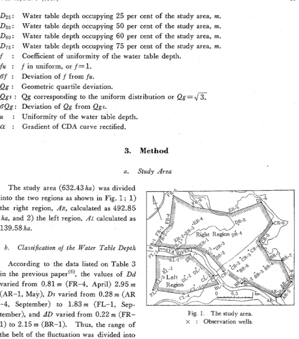
Methoda. Study Area
The study area (632.43 ha) was divided into the two regions as shown in Fig. 1; 1 ) the right region, AR, calculated as 492.85
ha, and 2) the left region, AL calculated as
139.58 ha.
b. Classzficatzon of the Water Table Depth
According to the data listed on Table 3 in the previous paper(6), the values of Dd
varied from 0.81 m (FR-4, April) 2.95 m
(AR-1, May), Ds varied from 0.28 m (AR -4, September) to 1.83 m (FL-1, Sep- tember), and AD varied from 0.22 m (FR- 1) to 2 1 5 m (BR-1). Thus, the range of
Fig 1 The study area x : Observation wells the belt of the fluctuation was divided into
six classes with a 0.5 m interval from 0.0 to 0.5 m to 2.5 to 3.0 m-depth. This classification was used to draw up the isobath maps shown in Figs. 2, 3, and 4, and it was also used to make up the Depth Area Curve, DAC, shown in Fig. 5.
T o make up the cumulative Depth Area Curve, CDAC, shown in Fig 6, the belt of fluctuation was classed into a cumulative six classes.
c. Isobath Map
From the values of Dd listed on Table 1 in the previous paper(8), we made up an isobath map of Dd by the usual method to construct the isobath map(''). We traced this isobath map on a lmm-section-tracing paper. to calculate the area between the two equi-depth lines of' the water table. We calculated the lmm2 into ha. Both methods, the poler planimeter and the
Tech.. Bull. Fac Agr. Kagawa Univ. mesh-counting methods were used.
4. Results and Discussion
4.1 Area Characteristics of Dd, Ds, and AD 4.1.1 Isobath Map of Dd
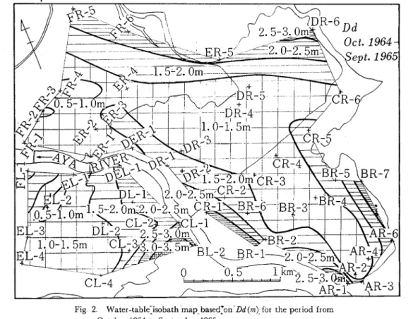
Fig. 2 shows the isobath map of Dd. From this figure, it is clear that the deep water-table depth of Dd appeared along the foot of the mountain side and the narrow strips near the right side of the Aya River and the upper part of the left region. From this figure, we made u p Table 1-A and Table 1-B.
Right Region: From the upper district to the lower district, a greater part of the region,
56.33 per cent (277.61ha) is occupied by the area having 1.0 to 1.5m water table depth of
Dd
Fig 2 Water-tableyisobath map based1on-Dd(m) for the period from October 1964 to September 1965
There are four areas making u p a sum of 143 55 ha having 1.5 to 2.0 m water table depth of Dd. This is 29 13 per cent of the region. Thus, the area having 1.0 to 2.0m water table
depth of Dd occupies 85.46 per cent of the region.
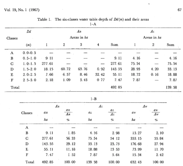
Vol 19, No. 1 (1967) 6 7 Table 1. The six-classes water table depth of Dd(m) and their areas
1-A
Classes Areas in ha Areas in ha
(m) 1 2 3 4 Sum 1 2 Sum - A 0 0-0 5 - - -
-
-
- - - B 0 5-1 0 9 11-
- - 9 11 4 16 - 4 16 C 1 0-1 5 277 61 - - - 277 61 75 54 - 75.54 D 1 5-2 0 18 15 60 72 63 76 0 92 143 55 28 93 4 20 33 13 E 2 0 - 2 5 7 6 6 6 5 7 8 4 6 3 2 4 2 5 5 1 1 1 8 7 2 0 1 6 1 8 8 8 F 2 5-3 0 2.18 1 09 3 43 0 77 7 47 7 87 - 7.87 Total 492 85 139 58-
AR A L A w aR-
-
aL a w Classes an An ax AL a 19-
Aw Total 492 85 100 00 139 58 100.00 632 43 100 003.43ha). and along the foot of the mountain, there are three small areas; 2.18ha (F-1), 1.09 ha (F-2), and 0.77 ha (F-4) The sum of them is 7.47 ha (1.52 per cent).
Left Region: T h e lower part of the region, that is 54.12 per cent or 75.54ha, is occupied by the area having 1.0 to 1.5m water table depth of Dd. In this area, around EL-2, there is a small area (4.16 ha, 2.98 per cent) having 0.5 to 1.0 m water table depth of Dd. There are two areas having 1.5 to 2.0 m water table depth of Dd, 28.93 ha (D-1), and 4.20 ha (D-2), and the sum 33.13 ha occupies 23.73 per cent of the region. Thus, 77.85 per cent of the region is occupied by the area having 1.0 to 2.0m water table depth of Dd.
Whole Study Area: 55.84 per cent of the study area (353.15ha) is occupied by the areas having 1.0 to 1.5m water table depth of Dd, and 27.94 per cent is occupied by 1.5 to 2.0~2,
thus, 83.78 per cent is occupied by 1.0 to 2.0m.
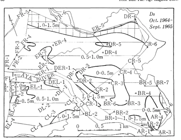
4.1.2 Isobath Map of Ds
Fig. 3 shows the isobath map of' D.s. From this figure, it is clear that the deep water-table depth of' Ds appear a t the foot of' the mountain side, in the narrow strips near the r.ight side of the Aya River and in the upper part of' the left region. From Fig. 3 , we made up Table
2-A and Table 2-B,.
Tech Bull Fac Agr Kagawa Univ
Fig 3 Water-table isobath map based on Dr ( m ) for the period from October 1964 to September 1965
Table 2 The four-classes water table depth of Dr ( m ) and their areas 2-A
Dr Ax A L
Classes Areas in ha Areas in ha
( m ) 1 2 3 4 5 Sum 1 2 3 Sum Total 492 85 139 58 An AI AT*. ax
-
U L au Classes an A R a~ A L a 14 -- A ~u A 7 7 42 15 71 8 38 6 00 85 80 13 57 B 327 43 66 43 113 69 81 45 441 12 69 7 5 C 85 21 17 29 16 73 11 99 101 94 16 12 D 2 79 0 57 0 78 0 56 3 57 0 56 Total 100 00 139.58 100 00 632 43 100 00cent (327.43 ha) of the region, and it spreads from the upper district to the lower district of the region as shown in Fig. 3. In this area, there four areas having 0.0 to 0.5m water table depth of Ds, making u p the sum of 77.42ha which is 15.71 per cent of the region (See Table 2-B). Five areas having 1.0 to 1.5m water table depth of Ds are distributed along the foot of the mountain and along the right side of the Aya River. Making u p the sum of
85.21ha which 17.29 per cent of the study area. Thus, the areas having 1.5m or less water-table depth of Ds occupied 99.43 per cent of the region.
Left Region: An area having 0.5 to 1.0m water table depth of Ds occupies 81.45 per cent (113.69 ha) of the region. In this area, there is a small area having 0.5 m or less water
-
table depth of Ds (8.38ha, 6.00 per cent). There are three areas having 1.0 to 1.5m water- table depth of Ds making u p the sum of 16.73 ha which is 11.99 per cent. Therefore, the sum of the areas having 1.5m or less water-table depth of Ds, 138.80 ha occupies 99.44 per cent of the region.Whole Study Area: As listed on Table 2-B, 69.75 per cent of the whole study area is occupied by the areas having 0.5 to 1.0 m water -table depth of Ds, and 16.12 per cent is 1.0
to 1.5m, 13.57 per cent is 0.5 m or less. Thus, the areas below 1.5 m water table depth of
Ds
occupy 99.44 per cent of the study area.
4.1.3 Isobath Map of AD
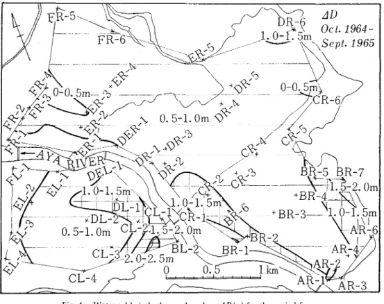
Fig. 4 shows the isobath map of AD. From this figure, it is clear that the deep water-table
Fig 4 Water-table isobath map based on 4 D ( m ) for the period from
70 Tech Bull Fac Agr Kagawa Univ depth of AD appears at the foot of the mountain side, in the narrow strips near the right side of the Aya River, and in the upper part of the left region. From Fig. 4 we made up Table 3-A and Table 3-B.
Right Regzon: An area having 0.5 to 1.0m water-table depth of AD occupies 83.14 per cent (409.76ha) of the region, and it spreads from the upper to the lower districts of the region. Along the right side of the downstream of the Aya River, there are two areas having
0.0 to 0.5m water table depth of AD, A-2 (15.27 ha) and A-3 (8.91 ha). There is also an area having the same water table depth of AD, A-1 (2.41 ha), near CR-6. The sum, 26.59 ha, is 5.40 per cent of the region. Along the right side of the upper stream of the Aya River, there are narrow belt-shape areas having 1.0 to 1.5m and more water-table depth of AD.
Also, along the foot of the mountain there are areas of 1.0 to 1.5m and more water-table depth of AD.
Left Regzon: The lower half of the region is occupied by two areas, having 0.0 to 0 5 m
and 0.5 to 1.0 m water -table depth of AD, making up the sum of 102 50 ha. Above the 0.5
to 1.0m area there is an area having 1.0 to 1.5m water table depth of AD (28.30ha, 20.28
per cent). Thus, the areas with less than 1.5 m water table depth occupy 93.71 per cent of the region.
Whole Study Area: As a whole study area, 97.94 per cent of the study area is occupied by the water-table depth of AD, with less than 1.5m.
4.2 Relationship Between D and aR, aL, and aw
4.2.1 D A Curves of Dd, Ds, and AD
From the data listed on Table 1-B, we. made up three DA curves of Dd as shown in Fig. 5. Similarly, from the data listed on Table 2-B and Table 3-B, we made up DA curves of Ds and AD as shown in the same figure respectively.
Rzght Region: From the figure, the modal depth mode(^), are obtained; for Dd, it is 1.0 aR
to 1 . 5 1 ~ ~ water table depth and the corresponding value of -
AR is 56.33 per cent: For Ds, aR
0.5 to 1.0 m depth and the corresponding value of -
AR is 66.41 per cent, and for AD, 0.5 aR
to 1.0 m depth and the corresponding value of -
AR is 83.14 per cent.
Left Regzon: The vaiues of Dmode are 1 ) for Dd, 1.0 to 1.5m water-table depth ar,d
U L U L
AL
--- is 54.12 per cent, 2 ) for Ds, 0.5 to 1.0m depth and
-
AL is 81.45 per cent, and 3) aL
for AD, 0.5 to 1.0m depth and -
AL is 62.26 per cent.
Whole Study Area: As a whole study area, the values of Dmode are 1 ) for Dd, 1.0 to
aw . a w
1.5m water-table depth and
-3%
is 55.84 per cent, 2 ) for Ds, 0.5 to 1.0m depth and -A w aw .
is 69.75 per cent, and 3 ) for AD, 0.5 to 1.0m depth and is 78.53 per cent of' the study area.
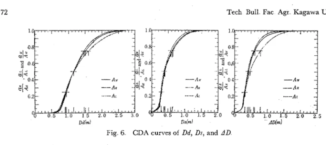
4.2.2 C D A Curves of Dd, Ds, and AD
From the data listed on Table 1-B, Table 2-B, and Table 3-B, we also drew u p Fig 6.
Vol 19, No 1 (1967) 7 1
Table 3 The five-classes water table depth of AD(m) and their areas
3-A 3-B
AD An At An an A L A w
az aw
Classes Areas in ha Areas in ha an --- An a= Ar aw A w
(m) 1 2 3 Sum 1 Sum ha % ha % ha %
-
A 0 0 - 0 5 2 4 1 1 5 2 7 8 9 1 26 59 1 5 5 9 1 5 5 9 2 6 5 9 5 4 0 1 5 5 9 11 17 42 18 6 6 7 B 0 5 - 1 0 4 0 9 7 6 - - 409 76 86 91 86 91 409 76 83 14 86.91 62 26 496 67 78.53 C 1 0-1 5 20 23 29 48 2 56 52 27 28 30 28 30 52 27 10 61 28 30 20 28 80 57 12 74 D 1 5-2 0 2 44 1 74 - 4 1 8 8 7 8 8 7 8 4 1 8 0 8 4 8 7 8 6 2 9 1 2 9 6 2 0 5 E 2 0-2 5 0 05 - -- 0 05 - - 0 05 0 01-
- 0 05 0 01 Total 492 85 139 58 492 85 100 00 139 58 100 00 632 43 100 00a
D(m)a
D (m)a
D (m) Fig 5 D 4 curves of Dd, DI, and 4D for the period from72 Tech Bull Fac Agr Kagawa Univ
Fig. 6 CDA curves of Dd, Dr, and AD
AD. The curves shown by the chainline are the values of the right region, the curves shown by the dotted line are the values of the left region, and the curves shown by the solid line are the values of the whole study area. These curves tell us the relationship between the cumulative water-table depth of Dd, Ds, and AD, and the area for the period from October
1964 to September 1965.
Table 4. Values of D,,, Dso, and D,,
Medzan Depth, Dmed, and D25 and D r 5 : From the curves shown in Fig 6, we obtained the values of the median depth, Dmed, or Dso, the water table depth occupying 50 per cent of t h ~ e ~ i o n . ( ~ ) The results are listed on Table 4. We also, obtained D25, and D ~ ~ " ) , from the same figure and the results are listed on the same table.
4 . 3 Uniformity of the Water Table Depth
4.3.1 Coeficient of' Unif'ormit,y, ,f
As a parameter defining the uniformity of the distribution of the water-table depth of Dd, we used the following equation (1);
1 If the value of'f equals 1, the water table depth is uniform. If' the value of , f ' equals ----,
3
the water table is of a uniform distribution which means the water table slopes linearly. T o get areas A and B for every curve of' Fig. 6, every curve was traced on a lmm-mesh tracing paper and the area was estimated by the mesh-counting method(2), and the values of
Vol. 19, No 1 (196'7) 73
f were obtained by using Eq. ( I ) . T h e results of the calculation using Eq. ( 1 ) is listed on Table 5. The values of f vary from 0.394 (AD in A L ) to 0.602 (Dd in AR).
T o find out the deviation of the value of f from f = l , we introduced the following equation,
Using Eq. (2), we calculated thc data listed on Table 5, and we obtained the values of 6f
as listed on the same table.
Table 5 Values off and of
-
Dd (m) D f (m) AD (m)
The values of dy vary from 39.8 per cent (Dd in AR) to 60.6 per cent (AD in AL). T h e data tell us that the water table depth of' Dd, D.s, and AD are not unifbrm. However, the depth of' Dd is closer to being a uniform ( f = 1 ) than unifrom distribution f
(,
=-2
,
whereas the depth of' D.r is closer to being a uniform distribution rather than unifrom.4.3.2 Uniformity, u
T o express the degree of uniformity of the water table depth, we used HAZEN'S method which is used to express the uniformity of'the grain-size d i s t r i b ~ t i o n ( ~ ) , and we introduced
into our case. Eq. (3) '
If the value of u equals I, the depth of the water table is unifrom. If' the value of u is larger than the water table depth is not uniform..
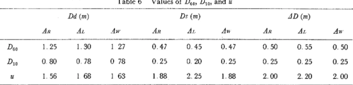
Using Eq. (3), we calculated the data, and we obtained the values of u as listed on Table
6. The values of u vary h a m 1.56 (Dd in AL.) to 2.25 (Ds in AR), thus, the water table depth is not uniform. However, Dd in AR is closer to being uniform than any values of' u on Table 6.
Table 6 Values of D,,, Dl,, and u
Dd (m) Dr (m) .4D (m)
74 Tech Bull.. Fac Agr. Kagawa Univ. This result coincides with the result obtained from Eq. (2).
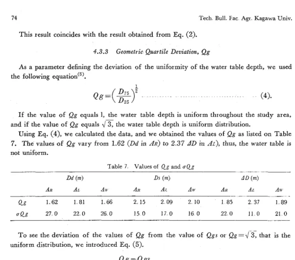
4.3.3 Geometric Quartile Deviation, Qg
As a parameter defining the deviation of the uniformity of' the water table depth, we used the following equation(5).
If the value of Qg equals 1, the water table depth is uniform throughout the study area, and if the value of Qg equals
4 3
the water table depth is uniform distribution.Using Eq. (4), we calculated the data, and we obtained the values of &g as listed on Table 7. The values of Qg vary from 1.62 (Dd in A R ) to 2,37 AD in Ar), thus, the water table is not uniform.
Table 7 Values of Qg and aQg
Dd (m) Dr (m) AD (m)
T o see the deviation of the values of Qg from the value of Qgs or Qg=d3, that is the uniform distribution, we introduced Eq. (5).
Using Eq. (5), we calculated the data on Table 7, and we obtained the values of 6Qg as listed on Table 7. The values of 6Qg vary from 11.0 per cent (AD in A L ) to 27.0 per cent
(Dd in AR). Thus, the water table depth of AD in AL is closer to the uniform distribution
throughout the data.
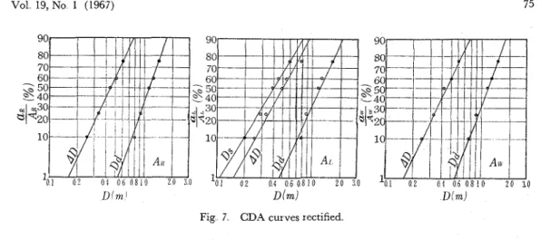
4.3.3 C D A Curve Rectified
T o see the gradient of the curves of the CDA curves shown in Fig. 6 , we rectified the curves to a logarithmic-normal distribution paper, and we drew up straight lines as shown in Fig. 7. Graph AR shows the curve rectified for the right region, similarly, graph AL for the
:(1
aLleft region, and AW for the whole study area. The axes of y are ---
--
is for AR,-
a w AL
for AL, and ---
A w for A w
),
and axes of x are D(m), the water table depth. One of thepurposes of the rectification is to find out an algebraic expression from the data on a straight line('). However, we used the rectification to find out the gradient of the straight lines.
Vol 19, No 1 (1967) 75
Fig 7. CDA curves rectified.
As the values of
a
increase to the 90'(a=
90°) the straight lines or the C D A curves rectified on the graphs become vertical to the x-axes. This means that the water table depth is uniform. As the values ofa
decrease, the water table is uniform distribution.Before using Eq. (6) we estimated
Table 8 Values of A
(
----:
I,
A ( D ) and aevery straight line as listed on Table
~ ( i )
A ( D ) a
Q
U.
Using Eq. (6), we calculated the Dd 7 2 2 5
Ax 2 88
data on Table 8 and obtained the AD 7 2 3 4 2. 12 values of a as listed on the same Dd 7 2 3 3 2 18 table. The values of
a
vary from A L Dr 7 2 4 2 1 72 1.72 (Ds in A L ) to 2.88 (Dd in AR). AD 7 2 3 9 1 85 Throughout the study areas, the val-Aiv Dd 7 2 2 6 2 77
ues of Dd are the largest. AD 7 2 3 4 5 2 09
5. Summary
T o find out the characteristics of the belt of fluctuation by means of the areal characteris- tics, we drew u p isobath maps of Dd, Ds, and AD. From these isobath maps, we constructed the DA and CDA curves, and we obtained the values of Dlo, D25, D50, Dso, and DT5 of Dd,
Ds, and AD for the right region, the left region and the whole study area. W e estimated the
uniformity of the water table depth of Dd, Ds, and AD for the study areas.
Using the logarithmic-normal distribution papers, we rectified the CDA curves into straight lines. From these straight lines, we also estimated the gradient of these lines,
a.
W e useda
to estimate the uniformity of the water table.T h e results of the study are as follows:
1) In the lowest stage of the water table or Dd, 55.84 per cent of the whole study area was occupied by the area having 1.0 to 1.5m-depth, and 27.94 per cent was occupied by 1.5 to 2.0m-depth. However, in the highest stage of the water table or Ds 69.75 per cent was of the 0 5 to l.0m-depth, and 16.12 per cent was of the 1.0 to 1,5m-depth. T h e belt of
76 Tech Bull Fac Agr Kagawa Univ fluctuation or AD with less than 1.5m was 97.94 per cent.
aw
2) The values of' Dmodc were 1) 1.0 to 1.5m-depth and -=55.84 per cent of the
aw Aw
whole study area for Dd, 2) 0.5 to 1.0m-depth and-=69.75 per cent for D.5, and 3) 0.5
aw Aw
to l.0m-depth and -= 78.53 per cent for AD. Aw
3) Coefficient of' uniformity or f ' that were estimated by Eq. (1) varied fiom 0..394 (AD in AL) to 0.602 (Dd inAR). The deviation of' the values of' f' from , f = l or qf' that were calculated by Eq. (2) varied fiom 39.8 per cent (Dd in AR) to 60.6 per cent (AD in AL).
Uniformity u that was calculated by Eq. (3) varied from 1.56 (Dd in AR) to 2.25 (D.s in AL). Geometric deviations Qg that were calculated by Eq. (4) varied from 1.62 (Dd in AR) to 2.37 (AD in AL.). The gradient of the CDA curves rectified or
a
that was calculated by Eq. (6) varied from 1.72 (Ds in AL.) to 2.88 (Dd in AR).4) Every water table is neither in uniform nor in uniform distribution. However, the water table of Dd in closer to the uniform than uniform distribution. The water table of Ds is closer to the uniform distribution than uniform.
6. Acknowledgements
The writers wish to thank Former Professor Dr. Hitoshi FUKUDA, and Associate Professor Dr. Hiroyuki OGATA both of Tokyo University for their encouragement.
A part of the expenditure was from the research fund donated by the Ministry of Educa- tion.
References
(1) BURROUS, W H : Grapl~ical Technicques for Engineering Computations 75-85, London, Mcmillan (1965)
(2) BURROUS, W H : zbzd
,
209-210(3) FUKUDA, K : Shallow-Ground Water in the Downstream Basin of the Aya River, V, Tech Bull Fa6 Agr Kagawa Univ,l8,211-216(1967) (4) FUKUDA, K : zbid ,216-221 (1967)
(5) FUKUDA, K : tbzd, 223-225 (1967)
( 6 ) FUKUDA, K
,
IZUISU, K,
MAEKAWA, 'I: Shal- low-Ground Water in the Downstream Basin of the Aya River, Kagawa Prefecture, VI, T e ~ hBull Fac Agr Kagawa Unzv
,
19, (1967) (7) FUKUDA, K,
Izursu, K,
MAEKAWA T : zbzd,(1967)
(8) FUKUDA, K, IZUISU, K
,
MAEKAWA, T : zbzd, (1967)(9) TERZAGH, K : Soil Mechanics in Engineering Practice, 21-22, Tokyo, Seventh Printings Charles E Tuttle Co (1965)
(10) TODD, D K : Ground-Water Hydrology, 66- 67, New York, John Willey & Sons Inc (1959)
Vol. 19, No. 1 (1967)
VII Isobath maps, D A
B
& U C D A curues fp 5 % 2 fzg-g
% & U%-E&T7k43Db9%akiC9L>T ( I )
Belt of fluctuation DiiiId, % 2 1; hf:&&8%%-&-F1k%T% S dZ 75 EJ @iZ %L )T&T7kR8%Bic
~ c 1 - c ~
6;t)liz L?:jS>6,c
~ % % T I ~ E B K J ~ ~ @ I % % : ? T .1) Dd (&X$i&T7k4), Dr (G&%T7kl&), % k U: 4D (= Dd-Dr) 8 Isobath maps Lj:. C ;hi2 k 5 & , Dd7Cd Aw (&&%) 0155 84% (353 15ha) db, D (&7;7kf3) $1 O d D d 1 5 m T d j 3 , 27 94 %$1 5 L D L 2 Om T d j s (Fig 2, %A73 Tables 1-A, 1-B) Dr 412, Aw 8 6 9 75% $0 5 L D L l Om ~ d j g , 16 12% 1 O d D b l 5m, 13 57% 5s D L 0 5m T, $&Ej A W 8 9 9 44% ;Sf D L ~ 5m Ti575 (Fig 3 $k U: Tables 2-A, 2-B) AD TI$, 97 94% D L 1 5m T d j 5 (Fig 4 %kjd 73 Tables 3-A, 3-B)
2) Isobath maps 7511; DA curtes G$i?+t: (Fig 5) Z ;hick 8 2 , Aw Dmode (Modal depth) [A, Dd KiM. LTC2, 1 OLDmodeL 1 5m T 2 K = 5 5 84% A w (aw Id Dmode h>&&575E@) 4 % 3, Dr 12% LTGd, 0 5 L D m o d e d l Om T d j - 7 4 , 2:=69 75 % T d j Z AD IC$$l.,LTIb, 0 5LDmodeLl.Om 4
==
A w A w
78 53% Tdj75.
3) DA curves jS> 1 ; g i Z CDA curves gt5j :j (Fig 6 ) Z ;hick 75 2, A w TI$. Dmed (Medzan depth,= DSo) Cd, 1 1 5 m ( D d ) , O 4 0 m ( D r ) , % k U : O 4 3 m ( A D ) T i 5 7 5 tL%, D l o , D z s , D s o % k 7 3 D75 b%+7': (Tables4 B k U : 5)
4) f
fa
(Coefficient of uniformity, Eq (1)) t2, A W T i t , 0 571 (Dd), 0 402 (Dr), $kU:O 451 (AD) T d j 3, of jg ( f = 1 ~ 1 1 ; 8 devzatzon, Eq (2)) Id, 43 0 % (Dd), 57 8 % (Dr) % & 0 54 9 % (AD) T d j 3 , DdA*
& 3 uniform i ~ j E<
, Dr Cdk 3 uniform distribution KjEt (Table 5) u I& (Eq (3)) ~ r > % T @ n b H & Ti575 (Table 6) Q.g I& (Fig (4)) Ib, 1 66 (Dd), 2 10 (Dr) 2510 1 89 (AD), 2 7: aQg I& (Eq (5)) lb, 26% (Dd), 16% (Dr), 21 0 % (AD) T d j 7 7 , Dr h f k 3 uniform distribution KjE (, Dd ;bhk 3%2 ;hit, f ll, u Q 2 ElB01%%%/irif. 3 1; iZ, CDA curves %E%!.fk (Fig 7) L, C ;h2 x-$42 0 gradients %$t;-f.dlJLt:aIE(Table8) 6 , _h2H&8@T'nl%%Lf:.