東北大学機関リポジトリTOUR

(1)

The effect of pollen exposure on economic

activity:Evidence from home scanner data

著者

Kuroda Yuta

journal or

publication title

DSSR Discussion Papers

number

114 page range

1-42

year

2020-05

URL

http://hdl.handle.net/10097/00127726

(2)

Data Science and Service Research

Discussion Paper

Discussion Paper No. 114

The effect of pollen exposure on economic activity: Evidence from home scanner data

Yuta Kuroda

May, 2020

Center for Data Science and Service Research Graduate School of Economic and Management Tohoku University 27-1 Kawauchi, Aobaku Sendai 980-8576, JAPAN

(3)

1

The effect of pollen exposure on economic activity:

Evidence from home scanner data

Yuta Kuroda

a

a Graduate School of Economics and Management, Tohoku University Sendai-Shi, Aoba-Ku, Kawauchi, 27-1, 980-8576, Japan

Email: [email protected]

Abstract

Although seasonal allergies caused by airborne pollen are detrimental to physical and mental health and impair daily activity, discussion on their social cost is scarce in the economics literature. Large amounts of airborne pollen can not only increase health care costs and reduce worker productivity, but also cause people to stay at home, thereby stagnating economic activity. This study uses daily purchase records from scanner data to investigate the effect of pollen exposure on consumption behavior. Exploiting the daily variation in the pollen counts at 120 observation stations in Japan, I find that consumption expenditure decreases by about 2% on days when airborne pollen is unusually high. A reduction in consumption due to pollen exposure is also observed in estimates using weekly and monthly panel data. This finding suggests that exposure to pollen may reduce total expenditure as opposed to delay spending. The results highlight the overlooked economic burden of pollen and seasonal allergies. Hence, they underline the importance of urban planning to reduce airborne pollen and health policy to deal with seasonal allergies.

Keywords: Seasonal allergies, Pollen, Consumption, Scanner data, Hay fever JEL classifications: Q51, D12, Q53, I10, E21, R11

(4)

2

1. Introduction

Seasonal allergy, also known as hay fever or pollinosis, is a common chronic condition and a global health problem (Bousquet et al., 2008). Seasonal allergy causes sneezing, nasal congestion, and itchy eyes, and its medications also bring about side effects such as sleepiness and lethargy (Jáuregui et al., 2009, Meltzer et al., 2012). The prevalence rates vary between country and region, but are generally 10% to 40% in developed countries, with an estimated 400 million sufferers worldwide (Greiner et al., 2011; Meltzer et al., 2012). Furthermore, numerous studies demonstrate that the prevalence is increasing (Caillaud et al., 2015; Linneberg et al., 2000; Nakae and Baba, 2010; Selnes et al., 2005) for a variety of reasons. Increases in temperature and precipitation due to global climate change increase pollen, which is the cause of seasonal allergy (Bajin et al., 2013; Shea et al., 2008; Todea et al., 2013; Zhang et al., 2015; Ziello et al., 2012). The urbanization and westernization of lifestyles also raise the prevalence of seasonal allergy (Kaneko et al., 2005; Krämer et al., 2010; Sakashita et al., 2010). Many developed countries are greening their cities to improve the air quality and landscape, which in turn leads to airborne pollen (Asero, 2002; Cariñanos and Casares-Porcel, 2011; Xu et al., 2016). Thus, since the burden of seasonal allergy can increase with economic activity, there is a need to study its social cost.

Despite the potential economic burden of seasonal allergy, economists pay little attention to pollen compared with pollutants. The medical and epidemiological literature indicates that seasonal allergy results in direct medical costs and indirect costs due to reduced labor productivity (Cardell et al., 2016; Hellgren et al., 2010; Lamb et al., 2006). However, these are not the only potential burdens of seasonal allergy. As with severe air pollution, pollen can also prevent people from going out (Graff Zivin and Neidell, 2009; Neidell, 2009) and affect their consumption behavior (Kang et al., 2019; Sun et al., 2019). High levels of airborne pollen make people stay at home, and the resulting loss of expenditure can be considered to be the economic

(5)

3

cost of pollen. However, the relationship between airborne pollen and consumption behavior remains unclear.

To bridge this gap in the body of knowledge, this study investigates the impacts of pollen exposure on consumption behavior. By combining detailed purchase records from 2013 to 2019 based on home scanner data with daily pollen counts collected at 120 monitoring stations throughout Japan, I analyze changes in consumer spending due to daily pollen variations. The main results provide evidence that consumer spending declines by about 2% on days when airborne pollen is unusually high (above the 95th percentile). Considering that consumption expenditure accounts for about 55% of GDP in Japan, this decline has serious implications. The estimates using weekly and monthly panel data also show a decrease in consumption expenditure for each additional day of high pollen, suggesting that pollen exposure causes shopping to be canceled rather than postponed. To the best of my knowledge, this is the first research to investigate the relationship between daily pollen exposure and consumption expenditure.

An important contribution of this study is that it presents novel evidence that pollen exposure impedes economic activity, thereby revealing the economic benefits of pollen reduction. First, understanding the social costs of pollen is important when formulating urban planning or greening policies, as considering the negative externalities caused by pollen in urban planning can improve social welfare. In addition, it can take a long time from planting to pollen production. In Japan, cedar was artificially planted nationally after World War II; cedar pollen is the biggest cause of seasonal allergies today. Some types of trees such as Japanese cedar take decades to start producing pollen, so ignoring it could be a huge burden in the future. Second, quantifying pollen costs contributes to the climate change literature. As climate change affects the production, dispersion, and allergen content of pollen (Ziska et al., 2019), my results reveal a potential novel channel through which climate change can affect social costs. Finally, the

(6)

4

effects of pollen should also be considered when using scanner data. High-frequency economic indicators using daily scanner data will become more common, and immediate policymaking using them could also increase in the future (De Haan and Van Der Grient, 2011; Melser, 2018). Although daily data are useful, they are susceptible to temporary exogenous variation. Considering the effects of pollen as well as daily weather and air pollution could thus allow for more accurate decision making.

The remainder of this paper is structured as follows. Section 2 explains pollen and seasonal allergies as well as related studies. Section 3 discusses the data and setting used in the study. Section 4 describes the empirical strategies. Section 5 presents the results, Section 6 explores their robustness, and Section 7 discusses the lasting effects of pollen. Finally, Section 8 concludes.

2. Background and related studies 2.1. Pollen and seasonal allergies

Seasonal allergy is a chronic disease caused by allergic pollen in the air. The causative plant and pollen season differ by country and region, but the symptoms are generally similar globally. Sufferers of seasonal allergies have an allergic reaction when they inhale airborne pollen. The most common reactions are allergic rhinitis such as sneezing, runny nose, and stuffy nose as well as allergic conjunctivitis such as itchy eyes and tears. In rare cases, asthma and atopy may also occur (Gonzalez-Barcala et al., 2013; Hanigan and Johnston, 2007; Sun et al., 2016). In the worst cases, it can cause bronchitis, bronchial asthma, pulmonary heart disease, and can even be life-threatening (Brunekreef et al., 2000; Weichenthal et al., 2016). In addition, allergy medications lead to side effects such as drowsiness, dryness, and lethargy (Jáuregui et al., 2009, Meltzer et al., 2012). These symptoms worsen sleep quality (Craig et al., 2004; Kremer et al., 2002; Santos et al., 2006), reduce cognitive performance (Bensnes, 2016; Marcotte, 2017),

(7)

5

increase absenteeism (Hellgren et al., 2010; Lamb et al., 2006), and sometimes lead to suicide (Stickley et al., 2017). Thus, seasonal allergies reduce people’s quality of life, affect their daily activities, and cause economic losses.

Seasonal allergy is a common disease, but the exact prevalence is difficult to ascertain because many sufferers use over-the-counter medications without visiting hospital or simply endure until the pollen season has passed because of the relatively mild and chronic symptoms. Several studies have estimated the annual per capita cost of seasonal allergies to be $600 to $1000, taking into account direct medical costs and indirect costs due to lost productivity (Cardell et al., 2016; Hellgren et al., 2010; Lamb et al., 2006). However, the burden of seasonal allergies may be underestimated.

A distinctive part of seasonal allergies is that sufferers’ performance and behavior are strongly influenced by airborne pollen count on that day. More patients visit the asthma emergency department (Erbas et al., 2012) and more over-the-counter medications for allergies are sold (Ito et al., 2015; Johnston et al., 2009) on days with high pollen counts. Bensnes (2016), Marcotte (2015), and Walker et al. (2007) show that high airborne pollen on exam days reduces students’ cognitive performance. Chalfin et al. (2019), who investigated pollen counts and crime, suggested that people may spend less time outdoors on high pollen days. They also found that not only outdoor crime but also indoor crime decreased on high pollen days, suggesting that high pollen may not only reduce outdoor activity, but also affect individual mood and behavior.

The results of Chalfin et al. (2019) suggest a new potential effect of airborne pollen. Similar to air pollution (Kang et al., 2019; Sun et al., 2019) and bad weather (Bloesch and Gourio, 2015; Parsons, 2001), the day’s airborne pollen count may be associated with daily expenditure. In other words, airborne pollen not only causes people to avoid going out, but may also decrease the desire to consume due to apathy and lethargy. Additionally, consumer spending could

(8)

6

decline to offset the higher medical costs caused by seasonal allergy. However, to the best of my knowledge, empirical evidence of the impact of daily pollen exposure on consumer spending is lacking.

2.2. Seasonal allergies in Japan

The main sources of seasonal allergies in Japan are cedar and cypress (Yamada et al., 2014; Yoshida et al., 2013). Cedar and cypress, which are not only suitable for the Japanese climate, but also have excellent characteristics for processing wood such as fast growth and easy shaping, were planted in large numbers during and after World War II when demand for materials was high but it was impossible to import timber. About 20% of Japan’s land is covered by artificial cedar and cypress forests (MAFF, n.d.), thereby playing important roles in public health by improving soil, air, and water quality. However, cedar and cypress begin to produce allergic pollen when they are about 30 years old.

Most pollen in Japan is distributed from February to April. Since pollen can be dispersed more than 100 kilometers away and can stay in the air for more than 12 hours, almost the entire area, even in sparsely forested cities, can be contaminated (Yamada et al., 2014). The regional prevalence rate is mostly 10–40% except for Okinawa1_{(Okuda, 2003; Sakashita et al., 2010;}

Yamada et al., 2014). Similar to the global trend, the prevalence rate in Japan is increasing steadily (Kaneko et al., 2005; Okano et al., 2012). Prevalence is particularly high in urban areas; in Tokyo, the prevalence rate reached 48.8% in 2016 (Tokyo Metropolitan Institute of Public Health, 2017), rising from 19.4% in 1996. As wearing protective masks as well as cutting down artificial forests and converting them to trees with less pollen have only marginal beneficial effects, a better understanding of the burden of seasonal allergies is necessary to help

1_{The climate of Okinawa prefecture, the southernmost remote island in Japan, is different than that in other}

prefectures. The prevalence of seasonal allergies is low because there is almost no pollen. Therefore, Japan’s 46 prefectures other than Okinawa are investigated in this study.

(9)

7

introduce effective policies and improve public health.

3. Data

To investigate the effect of daily airborne pollen count on consumption behavior, this study uses a combination of three types of data: pollen, weather, and individual purchases. The data period runs from February to June (pollen season) of each year, from 2013 to 2019. Data on air pollution are only used to check the robustness of the results because the available period is short (from 2013 to 2017).

3.1. Airborne Pollen

Daily pollen data were obtained from the pollen observation system (Hanakosan) operated by the Ministry of the Environment. There are 120 pollen monitoring stations in Japan, operating from February to May each year (until June in Hokkaido). Figure 1 shows the locations of pollen observation stations that except for sparsely populated areas cover most Japanese cities. Automatic pollen monitors in each station report the pollen count per cubic meter every hour.2_{The measured pollen count is automatically published on the website of the}

Ministry of the Environment to allow allergy sufferers to make decisions about medication use and outdoor activities based on real-time pollen information.

Table 1 shows the descriptive statistics. The mean pollen count is 43.327 and the standard deviation is 252.918, indicating that the variance is large.3_{This study uses the effect of pollen}

thresholds following the literature (Chalfin et al., 2019; Ito et al., 2015; Marcotte, 2015;

2_{There is no distinction between cedar and cypress because of their close properties. There are some}

deficiencies in the data due to equipment failure, data communication errors, or unusual yellow sand.

3_{The maximum pollen count is 66403.792, which may seem like an outlier. This value is the maximum for}

2013, but the maximum for the other years is around 2000 to 7000. However, the Ministry of the Environment reports that outliers are excluded before the release of the data. Hence, this study treats this value as a non-outlier. In any case, the main analysis uses dummy variables, so there is no major impact.

(10)

8

Sheffield et al., 2011). A day when the airborne pollen count is in the 95th percentile (158.167) or higher is defined as a high pollen day. Therefore, the main analysis captures the effect of extreme pollen counts. This is reasonable because the medical and epidemiological literature shows that symptoms of seasonal allergies can rise sharply with increasing pollen counts and flatten above the threshold (Caillaud et al., 2014; Erbas et al., 2007; Johnston et al., 2009). In addition, using the same threshold for all the monitoring stations is not problematic because, as mentioned in the previous section, pollen trees are distributed nationally and the variance of the average pollen count at each monitoring station is small.

Figure 1. Pollen monitoring stations in Japan

Note: The black rhombus symbols represent pollen monitoring stations. Source: Ministry of the Environment. ◆ Monitoring station

Longitude

La

titu

(11)

9

Table 1. Descriptive statistics

Note: Home scanner and air pollution data are aggregated for each pollen station within 15 km. The details of pollen-related goods are given in Appendix A. The number of observations is the number of pollen stations multiplied by the number of observation days minus the number of days when pollen data are missing.

3.2. Weather

As daily weather has a huge impact on consumer behavior (Bloesch and Gourio, 2015; Parsons, 2001), it must be controlled for. The weather data are obtained from the Automated Meteorological Data Acquisition System (AMeDAS) operated by the Japan Meteorological Agency. Pollen data and weather data can be matched one-to-one because pollen monitoring stations are intentionally located near AMeDAS stations. The variables used are a rain dummy (taking one when precipitation per hour is 15 mm or more), temperature (°C), and wind speed (m/s) (see Table 1). Intuitively, pollen counts are likely to be strongly influenced by rain;

Mean Std. Dev Minimum Maximum Pollen and weather

　Pollen count 43.327 252.918 0 66403.792

　High pollen day dummy 0.050 0.218 0 1

　Rain dummy 0.365 0.481 0 1

　Average temperature (°C) 13.286 7.250 -16 30.150

　Average wind speed (m/s) 2.555 1.345 0 15.650

Daily home scanner data

　Total in-store purchases 107519.750 170719.621 0 1830594

　Number of monitors purchased 68.894 110.525 0 844

　Total in-store purchases per monitor 1599.797 727.673 0 30407 　Total online and mail order purchases 11401.165 23078.241 0 902713 　Total purchases of pollen-related goods 1179.982 2552.407 0 49742 Air pollution 　Average PM25 (μg/m3) 14.389 8.198 0 86.028 　Critical PM25 dummy 0.101 0.301 0 1 　Average SO2 (ppm) 1.835 1.742 0 63.297 　Critical SO2 dummy 0.001 0.025 0 1 　Average NOX (ppm) 13.303 9.847 0 340.500

Number of pollen monitoring stations Number of observation days

Observations

120 98361

(12)

10

however, the weather has a small impact on pollen counts in reality (D’Amato et al., 2007). Consistent with the results of Chalfin et al., (2019), the R-squared value is only 0.06 when regressing pollen counts on the weather variables and all the other fixed effects using the data in the main analysis.

3.3. Home scanner data

To measure daily consumption expenditure, I use home scanner data called Quick Purchase Report (QPR) from Macromill. This dataset aims to provide detailed marketing information by constructing nationally representative panel data on consumers’ buying behavior. Since 2011, about 30,000 monitors4_{provided with barcode readers have reported daily purchasing data.}

Monitors scan all barcoded items purchased each day using handheld scanners and report the code, price, and quantity of each product. This dataset contains rich personal information about the monitors, including ZIP codes, age, income, and family structure, which is updated annually. Based on the ZIP code, I can combine the QPR data with the pollen station.5_{In addition, the}

QPR data include detailed information such as the date and time of the scan and location of the purchase (e.g., supermarket, mail order, vending machine) as well as the product name. An important feature of the QPR data is their high representativeness. Monitors are selected to ensure they represent the regional gender, age, marital status, and family structure shares based on the census. In addition, monitors are incentivized to scan correctly using rewards, and monitors who do not regularly scan are forced to leave; hence, the data are highly reliable.

However, as Leicester (2013), who compared home scanner data with other household survey data, pointed out, there are several problems with home scanner data. The most serious

4_{The QPR has maintained a sample size of about 30,000, replenished with individuals with similar}

characteristics when monitors drop out. Thus, it mitigates the problem of sample attrition, which is a serious shortcoming of daily purchasing data.

(13)

11

is that the QPR data do not capture all household expenditure. Items without a barcode such as perishables, cars, and properties are not included in the data. Further, even if a barcode is attached, some products such as imported products cannot be used for the analysis because the unit price is unknown. Therefore, the consumption expenditure used in this analysis is less than the actual value. In addition, the monitor must scan every day, so the sample may be biased toward industrious people. However, such deficiencies and biases are likely to be uncorrelated with pollen exposure and seasonal allergies, and should not seriously bias the estimates.

In the main analysis, the data are used at the aggregate level of each pollen monitoring station.6_{The distance from the center of the ZIP code of the monitor to the nearest pollen}

monitoring station is calculated, and the QPR data are connected to the pollen and weather data. In the main estimation, data from monitors living within 15 km of the pollen monitoring station are aggregated and used as the consumption activity data in the area around the station. For each pollen monitoring station, I use the following daily information: total in-store purchases, number of monitors making purchases of at least one yen, per capita in-store purchases, total online and mail order purchases, and total purchases of pollen-related products.7_{Table 1}

presents the descriptive statistics.

3.4. Air pollution

As with weather, air pollution levels can affect outdoor activities (Kang et al., 2019; Sun et al., 2019) and airborne pollen counts (D’Amato et al., 2007; Yamada et al., 2014). Therefore, air pollutants should be used as a control. The data on air pollutants are obtained from the National Institute for Environmental Studies. There are more than 2,000 automatic air quality

6_{Another technical problem is that because of the huge sample size, it is difficult to control for the}

monitor-level fixed effects in the monitor’s daily data and make estimates that account for the non-linearities caused by the many “zeros” (i.e., days when the monitor does not go shopping).

(14)

12

monitors in Japan, each reporting hourly airborne pollutants. In this study, air pollution is defined as the air quality at each pollen monitoring station (i.e., the average daily value reported by the air quality monitors within a certain distance of each pollen station). Unlike the pollen, weather, and purchasing data, the air pollution data are only available from 2013 to 2017. Therefore, they are not used in the main analysis, only in the robustness check.

Particulate matter (PM25, μg/m3), sulfur dioxide (SO2, ppb), and nitrogen oxides (NOX, ppb)

are used as the air pollution variables. Each pollutant is used not only as a value, but also as a dummy variable that takes one if it is above the critical threshold defined by the World Health Organization (WHO) (Bensnes, 2016). The threshold for PM25 and SO2 is 25 or more per hour

and 20 or more per hour, respectively (WHO, 2005). NOX is only used linearly because there

is no defined threshold. Table 1 shows the descriptive statistics of the pollutants used in the estimates.

4. Empirical strategies

To investigate the effects of pollen exposure on consumption expenditure, I estimate the following model:

𝑃𝑃𝑖𝑖𝑖𝑖𝑖𝑖𝑖𝑖 = 𝛼𝛼 + 𝛽𝛽𝑃𝑃𝑃𝑃𝑃𝑃𝑃𝑃𝑃𝑃𝑃𝑃𝑖𝑖𝑖𝑖𝑖𝑖𝑖𝑖+ 𝛾𝛾𝑋𝑋𝑖𝑖𝑖𝑖𝑖𝑖𝑖𝑖+ 𝑆𝑆𝑖𝑖 + 𝑌𝑌𝑖𝑖 + 𝑀𝑀𝑖𝑖 + 𝐷𝐷𝑖𝑖 + 𝑊𝑊𝑖𝑖𝑖𝑖+ 𝑍𝑍𝑖𝑖𝑖𝑖+ 𝜀𝜀𝑖𝑖𝑖𝑖𝑖𝑖𝑖𝑖 (1) where, 𝑃𝑃𝑖𝑖𝑖𝑖𝑖𝑖𝑖𝑖 represents consumption behavior in the catchment of pollen monitoring station 𝑖𝑖 on day 𝑑𝑑, month 𝑚𝑚, and year 𝑦𝑦.8_{In the main analysis, consumption behavior is proxied}

by total in-store purchases. 𝑃𝑃𝑃𝑃𝑃𝑃𝑃𝑃𝑃𝑃𝑃𝑃𝑖𝑖𝑖𝑖𝑖𝑖𝑖𝑖 is a dummy variable that indicates whether pollen is above the threshold and 𝛽𝛽 is the coefficient of interest.9_𝑋𝑋

𝑖𝑖𝑖𝑖𝑖𝑖𝑖𝑖 is a control vector that

8_{One concern with home scanner data is the timing of the scan. If the timing of the scan is after midnight,}

the purchase amount is recorded on the next day. Therefore, I also analyzed purchases made before 8 a.m. on the next day as being purchases for that day (except for purchases made at 24-hour convenience stores and vending machines). The results are similar to the main results (see Appendix B).

(15)

13

includes typical weather conditions such as daily average temperature, wind speed, and precipitation. For the robustness checks, air pollution levels are also included in 𝑋𝑋𝑖𝑖𝑖𝑖𝑖𝑖𝑖𝑖. 𝑆𝑆𝑖𝑖, 𝑌𝑌𝑖𝑖, 𝑀𝑀𝑖𝑖, and 𝐷𝐷𝑖𝑖 are the fixed effects of the pollen monitoring station, year, month, and day, respectively. 𝑊𝑊𝑖𝑖𝑖𝑖 and 𝑍𝑍𝑖𝑖𝑖𝑖 are the interaction of the station-year and station-month fixed effects, respectively, controlling the station-specific time trends. This allows us to address local economic trends and seasonality. To account for the serial correlation of the errors, standard errors are clustered at the station-year-month level. Controlling for the fixed effects in such detail allows me to identify the impact of exogenous variation in pollen on consumption behavior.

To better understand the impact of pollen on purchasing behavior, I also make estimates using dependent variables other than total in-store purchases. First, the number of people who went out shopping is used as the dependent variable to examine whether the increase in pollen decreases outdoor activities. Second, to ensure that the results are not driven by the number of monitors assigned to each pollen monitoring station, I use the purchase amount per monitor. Third, using online and mail order shopping expenditure, I confirm that allergy symptoms caused by airborne pollen do not affect the accuracy and frequency of home scanner data. Since online shopping can be ordered without going out and delivery usually takes a few days, it cannot be affected by the pollen on that day. If airborne pollen affects scanning behavior rather than purchasing behavior, then spending on online and mail order shopping will also decrease. Finally, I investigate pollen-related goods to confirm whether people’s behavior is affected by pollen. Since clinical studies such as Johnston et al. (2009) and Yamada et al. (2014) show that medication, masks, and glasses sell well on high pollen days, I define such products as pollen-related goods. The specific definitions are given in Appendix A.

some differences in significance levels, the results consistently show the negative effect of pollen on consumption. This is also consistent with the relationship shown in the medical literature that it flattens when the threshold is exceeded.

(16)

14

When considering the economic burden of pollen, the key question is whether the decline in consumption will bounce back. Although bad weather and air pollution have a negative impact on outdoor activities and consumption, this may simply be a postponement (Bloesch and Gourio, 2015; Graff Zivin and Neidell, 2014; Sun et al., 2019). In other words, outdoor activity may be postponed while the bad conditions continue and then rapidly increase when they are over. This suggests that the negative effects of high pollen days are transitory and have no serious impact on the economy. However, it is difficult to verify the degree to which the economy bounces back from continuously bad pollen conditions. Since clear thresholds are lacking, it is hard to state concretely that the high pollen period is over. Moreover, pollen can affect sufferers the next day because allergy symptoms may not recover after one day and pollen can stay on clothes and indoor surfaces. Therefore, weekly and monthly data are estimated using the average pollen level and number of high pollen days. If people avoid going out on high pollen days and instead shop on low pollen days, then no negative effects of high pollen days should be observed at the weekly or monthly level. Conversely, if there is no bounce back effect, the number of high pollen days at the weekly or monthly level can have a negative effect.10

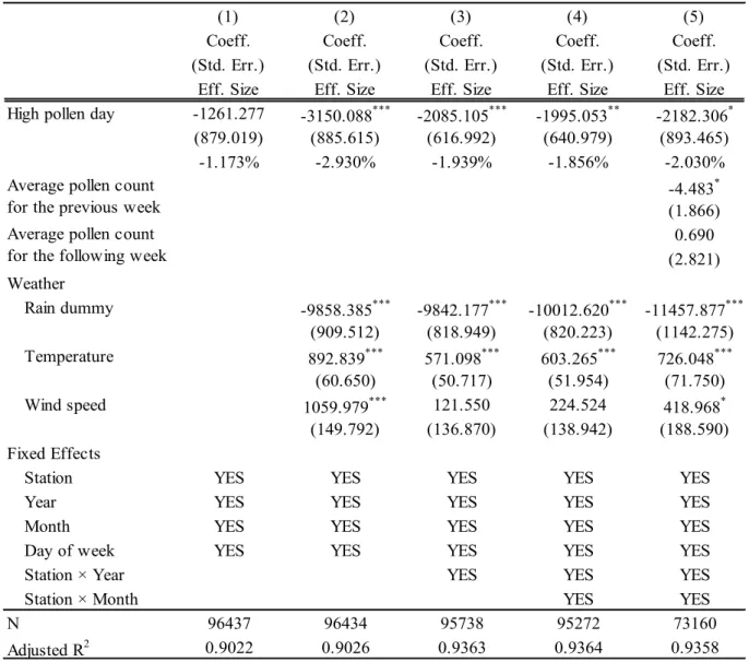
5. Main results

Table 2 presents the estimates of the impact of pollen exposure on in-store consumption expenditure. The treatment variable in each row is a dummy variable that takes one if the daily pollen count of a given monitoring station on a given day exceeds the 95th percentile (158.167). Each column reports the coefficients, their standard errors, and, for the variable of interest, the effect size as the percentage change in the dependent variable relative to its mean. Column (1)

10_{All the major analyses were performed at the level of pollen monitoring station, but weekly and monthly}

data were also used at the monitor level to confirm the robustness of the main results (see Appendix D and Appendix E).

(17)

15

shows the results estimated by controlling for only the basic fixed effects. When weather is not controlled for, there is no significant relationship between high pollen days and consumption expenditure. This is expected considering that the weather affects both consumption behavior and pollen dispersal, and this result emphasizes the need to control for the weather. Column (2) uses a specification with additional controls for weather conditions. The results show that consumer spending falls by 2.93% on high pollen days. Moreover, rainy days significantly reduce consumption, which is consistent with previous research (Parsons, 2001) and common sense. Columns (3) and (4) show the results with additional controls for the station-year and station-month fixed effects, respectively. Controlling for the time-fixed effects at the monitoring station level can reduce the bias caused by differences in the trends in the local climate, economic activity, and other unobserved factors. The results show that high pollen days significantly reduce consumer spending by about 1.9%. Column (5) additionally controls for the average pollen count in the weeks before and after the observation day to account for the effect of airborne pollen on adjacent days, which can affect purchasing behavior on the day in question. Column (5) indicates that even when controlling for pollen counts on adjacent days, there is no noteworthy change in the effect of high pollen days. It is also plausible that higher pollen levels in the previous week would slightly decrease consumer spending.

Hence, the main results show that regardless of the specification, store spending falls significantly on high pollen days. The effect size is 2–3%, in line with the findings of related studies that show that restaurant visitors decrease by about 4% on days with severe air pollution (Sun et al., 2019) and Citibike trips decrease by about 4% on days with high pollen counts (Chalfin et al., 2019).

(18)

16

Table 2. Effects of daily high pollen on consumption expenditure in stores

Note: *, **, and *** indicate statistical significance at 5%, 1%, and 0.1%, respectively. The effect size indicates the percentage change in the dependent variable relative to its mean on a high pollen day. Standard errors are adjusted for clustering at the station-year-month level.

(1) (2) (3) (4) (5)

Coeff. Coeff. Coeff. Coeff. Coeff.

(Std. Err.) (Std. Err.) (Std. Err.) (Std. Err.) (Std. Err.) Eff. Size Eff. Size Eff. Size Eff. Size Eff. Size High pollen day -1261.277 -3150.088*** _-2085.105*** _-1995.053** _-2182.306*

(879.019) (885.615) (616.992) (640.979) (893.465) -1.173% -2.930% -1.939% -1.856% -2.030% -4.483* (1.866) 0.690 (2.821) Weather 　Rain dummy _-9858.385*** _-9842.177*** _-10012.620*** _-11457.877*** (909.512) (818.949) (820.223) (1142.275) 　Temperature 892.839*** _571.098*** _603.265*** _726.048*** (60.650) (50.717) (51.954) (71.750) 　Wind speed _1059.979*** _121.550 _224.524 _418.968* (149.792) (136.870) (138.942) (188.590) Fixed Effects

　Station YES YES YES YES YES

　Year YES YES YES YES YES

　Month YES YES YES YES YES

　Day of week YES YES YES YES YES

　Station × Year YES YES YES

　_{Station × Month} _YES _YES

N 96437 96434 95738 95272 73160

Adjusted R2 _0.9022 _0.9026 _0.9363 _0.9364 _0.9358

Average pollen count for the previous week Average pollen count for the following week

(19)

17

6. Robustness checks

The main results are robust even when controlling for the various fixed effects discussed above. However, this section provides a series of robustness checks to address concerns about the main analysis, such as the composition of the sample and use of arbitrary thresholds.

6.1. Changing the explained variable

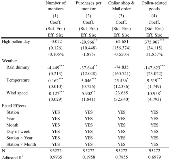
In this section, estimates with altered explained variables are conducted to investigate how people’s behavior changes on high pollen days. Table 3 shows the results for different explained variables using the specification in column (4) of Table 2. Unless otherwise specified, this specification is used for all the subsequent estimations. Column (1) uses the number of monitors who purchased something in a store that day as the dependent variable. The results show that high pollen has no significant effect on the number of people who make purchases, which is somewhat unexpected considering that outdoor activities may be hampered by airborne pollen. One explanation is that people spend less time outside on high pollen days, rather than not going outside at all. For example, on a high pollen day, people might buy the essentials at a nearby convenience store instead of going to a suburban shopping mall or touring multiple stores.11

Column (2) presents the results using in-store purchase amount per monitor, showing that high pollen days significantly reduce per capita consumption expenditure, with effect sizes similar to the aggregated consumption expenditure in Table 2. This indicates that the main results are not sensitive to the number of monitors assigned to each monitoring station. Column (3) uses expenditure on goods purchased without going out, such as online and mail order

11_{Regrettably, the distance between the monitor’s residence and place of purchase is not available from the}

data. To investigate outdoor activities, an analysis was conducted using the differences between weekdays and holidays. Although many people must go out on weekdays for work, holiday outings are arbitrary, suggesting that pollen may have a greater impact on outdoor activity in holidays. However, the results of the analysis showed no significant difference between weekdays and holidays.

(20)

18

shopping, as the dependent variable. As expected, online and mail order shopping is not significantly affected by high airborne pollen, emphasizing that the main results are not driven by changes in scanning behavior. Column (4) shows that spending on pollen-related goods increases significantly by about 32% on days when pollen is high. This exceptionally large effect presents evidence that people respond sensitively to pollen exposure.

Table 3. Effects of daily high pollen on other explained variables

Number of

monitors Purchases permonitor Online shop &Mail order Pollen-relatedgoods

(1) (2) (3) (4)

Coeff. Coeff. Coeff. Coeff.

(Std. Err.) (Std. Err.) (Std. Err.) (Std. Err.) Eff. Size Eff. Size Eff. Size Eff. Size High pollen day -0.072 -29.966** _-62.681 _375.907***

(0.126) (10.448) (156.374) (34.115) -0.105% -1.87% -0.550% 31.857% Weather 　Rain dummy -4.449*** _-37.644** _-74.835 _-147.823*** (0.213) (12.048) (160.741) (23.022) 　Temperature 0.162*** _5.046*** _25.436* _9.519*** (0.010) (0.726) (12.336) (1.749) 　Wind speed _-0.127*** _5.902** _23.685 _10.958* (0.029) (1.841) (32.640) (4.793) Fixed Effects

　Station YES YES YES YES

　Year YES YES YES YES

　Month YES YES YES YES

　Day of week YES YES YES YES

　Station × Year YES YES YES YES

　_{Station × Month} _YES _YES _YES _YES

N 95272 95272 95272 95272

(21)

19

6.2. Data composition

One potential concern with the main results is how the dataset is created. In the main analysis, monitors are aggregated by pollen monitoring station, but the distance from the station is decided arbitrarily. While using monitors close to a station can reduce measurement errors for pollen exposure, it can also lead to bias by reducing the number of monitors aggregated. Columns (1)–(5) of Table 4 show the results using monitors living within 5, 10, 20, 25, and 30 km of a pollen monitoring station, respectively.12_{Column (6) also shows the estimation results}

using the data generated by assigning all monitors to the nearest pollen monitoring station. Despite the wide variation in the number of monitors aggregated, from about 13,700 to about 66,700, the effects of high pollen days are negative, significant, and their sizes are remarkably consistent in all the columns, confirming that the main results are not sensitive to the distance at which the monitors are aggregated.

12_{The data used in the main analysis are from monitors living within 15 km of a pollen monitoring station,}

(22)

20

Table 4. Estimates when changing the monitor catchment area

Monitors within 5 km Monitors within 10 km Monitors within 20 km Monitors within 25 km Monitors within 30 km Full sample (1) (2) (3) (4) (5) (6)

Coeff. Coeff. Coeff. Coeff. Coeff. Coeff. (Std. Err.) (Std. Err.) (Std. Err.) (Std. Err.) (Std. Err.) (Std. Err.)

Eff. Size Eff. Size Eff. Size Eff. Size Eff. Size Eff. Size High pollen day -409.748* _-1258.720** _-2225.964** _-2516.903** _-2622.737** _-2788.157***

(206.295) (437.871) (748.260) (789.188) (809.036) (838.034) -1.310% -1.721% -1.715% -1.786% -1.757% -1.676% Weather 　Rain dummy -2549.196*** _-6619.283***_-12085.127***_-13057.422***_-13644.979***_-14553.022*** (243.810) (554.598) (964.223) (1033.277) (1060.811) (1098.126) 　Temperature 146.355*** _391.308*** _744.026*** _823.355*** _883.805*** _948.884*** (16.426) (35.158) (61.790) (65.674) (67.505) (70.089) 　Wind speed 47.094 97.900 194.195 179.625 133.807 159.180 (44.586) (95.804) (166.556) (178.771) (186.045) (196.487) Fixed Effects

　Station YES YES YES YES YES YES

　Year YES YES YES YES YES YES

　Month YES YES YES YES YES YES

　Day of week YES YES YES YES YES YES

　Station × Year YES YES YES YES YES YES

　Station × Month YES YES YES YES YES YES

# of aggregated

monitors 13705 32151 54581 58485 61302 66671

N 90339 94007 95867 95867 95867 95985

(23)

21

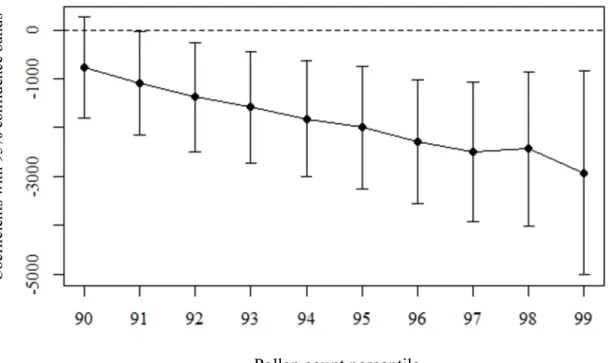
6.3. Pollen threshold

The main analysis defines a high pollen day as a day with a pollen level in the 95th percentile or higher, but this is also arbitrarily determined. Here, I re-estimate the specification in column (4) of Table 2 by varying the threshold for high pollen days to each percentile from the 90th to 99th percentiles. Figure 2 illustrates that the impact increases as the threshold rises. Naturally, as the threshold increases, the number of days corresponding to it decreases, and thus the precision of the estimates falls. This indicates that the main results are not sensitive to threshold changes.

Figure 2. Sensitivity of the threshold for high pollen days

Note: Each point represents a coefficient for a high pollen day defined as a pollen level higher than the percentile indicated by the value on the horizontal axis. The confidence interval around the point estimate reflects the 95% confidence interval. The other control variables are the same as in column (4) of Table 2, with the rain dummy, mean temperature, and mean wind speed as well as the fixed effects of the pollen monitoring station, year, month, day, station-year, and station-month. Standard errors are adjusted for clustering at the station-year-month level.

Pollen count percentile

C oe ffi ci en ts w ith 95% c on fid enc e ba nd s

(24)

22

6.4. Effects of air pollution

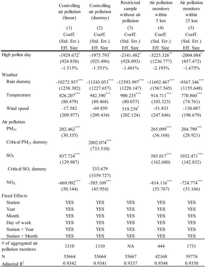
A critical concern with this study’s identification strategy is that other variables that correlate with both daily pollen counts and purchasing behavior affect the results. Since pollen dispersal is a natural phenomenon, such variables are unlikely to exist other than weather, but air pollution could be a problem. If the main results are driven by a third factor such as air pollution, the explanatory power of pollen could be markedly reduced or disappear when controlling for the air pollution variables.

To address this concern, I re-estimate controlling for the air pollution variables. Columns (1) and (2) of Table 5 consider the air quality of each pollen monitoring station to be the average value of the pollutant level reported by the air pollution monitors within 15 km of each station. Column (1) includes the pollution variables as linear and column (2) includes them as dummies that take one if they are above the critical threshold defined by the WHO. However, only NOX

is inputted as linear in both columns because the threshold is undefined. The results show that even after controlling for the air pollution variable, the effect of high pollen days on store consumption expenditure remains negative and significant. There is a slight decrease in the effect size compared with the main results, but this may be due to a decrease in the sample period. Column (3) shows the results using the same sample from 2013 to 2017, but excluding the variable on air pollution, to check the impact of the shorter sample rather than air pollution. The effect size in column (3) is slightly less than that in the main results in Table 2, suggesting that the impact of controlling for air pollution is not considerable. Finally, columns (4) and (5) use the average pollution levels reported by air pollution monitors within 5 km and 25 km of a pollen monitoring station, respectively to ensure that the results are not sensitive to how the pollution variables are generated. Although the effect size changes because of the change in the number of available pollen monitoring stations, both coefficients of interest are negative and significant, indicating that the results are not sensitive to the way the pollution variables are

(25)

23

generated. The results indicate that pollen has an effect independent of air pollution, enhancing the credibility of the identification strategy used in this study.

(26)

24

Table 5. Estimates when controlling for air pollution

Controlling air pollution (linear) Controlling air pollution (dummy) Restricted sample without air pollution Air pollution monitors within 5 km Air pollution monitors within 25 km (1) (2) (3) (4) (5)

Coeff. Coeff. Coeff. Coeff. Coeff.

(Std. Err.) (Std. Err.) (Std. Err.) (Std. Err.) (Std. Err.) Eff. Size Eff. Size Eff. Size Eff. Size Eff. Size High pollen day -1929.672* _-1975.793* _-2141.482* _-3223.326** _-2004.084*

(924.830) (925.496) (928.093) (1236.777) (857.472) -1.515% -1.551% -1.681% -2.193% -1.675% Weather 　Rain dummy -10272.937*** _-11243.053*** _-12593.997*** _-11692.467*** _-9367.346*** (1238.302) (1227.657) (1220.147) (1567.545) (1155.648) 　Temperature 826.207*** _942.390*** _900.235*** _914.711*** _770.860*** (80.479) (80.468) (80.037) (103.323) (74.761) 　Wind speed -17.582 -69.859 519.239* _-51.833 _-130.087 (209.977) (209.434) (202.124) (247.846) (198.679) Air pollution 　PM25 202.462*** 265.099*** 204.790*** (30.335) (36.168) (28.921) 　Critical PM25 dummy 2802.074*** (733.510) 　SO2 837.724*** 585.017*** 1032.471*** (129.987) (162.680) (142.832) 　 Critical SO2 dummy 333.679 (3359.727) 　NOX -669.092*** -585.109*** -814.116*** -724.774*** (50.144) (45.954) (55.767) (53.166) Fixed Effects

　Station YES YES YES YES YES

　Year YES YES YES YES YES

　Month YES YES YES YES YES

　Day of week YES YES YES YES YES

　Station × Year YES YES YES YES YES

　Station × Month YES YES YES YES YES

# of aggregated air

pollution monitors 1310 1310 NA 444 1731

N 55664 55664 55667 42168 59776

(27)

25

7. Transitory vs. lasting effects

To understand the economic impact, it is important to show whether the above-described negative effects of high pollen are lasting or transitory. One possible concern is that the decline in consumption due to high pollen may simply be a postponement, as studies of pollution and bad weather have shown (Bloesch and Gourio, 2015; Graff Zivin and Neidell, 2014; Sun et al., 2019). If consumption simply bounces back, the bounce back effect would cancel out the decline in consumption expenditure and pollen would have no lasting negative impact on the economy. High pollen usually does not continue for more than a few days; hence, if there is a bounce back effect, no negative effects of pollen should be observed at the weekly or monthly level. Alternatively, people might use online or mail order shopping instead of going out on a high pollen day. Because of the characteristics of online and mail order shopping, daily level data cannot analyze the impact of pollen. However, by using data at the weekly or monthly level, an alternative relationship between online and offline shopping due to high pollen levels may be observed. If the number of high pollen days in a week or month increases online consumption, the impact on total consumption expenditure may be limited, because pollen only changes the way of consumption. To determine whether the effects of pollen are transitory, this section thus examines in-store and online expenditure, using data aggregated at the weekly and monthly levels.

Table 6 shows the results using weekly data. In columns (1) and (2), the dependent variable is weekly in-store consumption expenditure and the control variables are the number of rainy days, average temperature, and average wind speed as well as the fixed effects of the pollen monitoring station, year, week, and station-year. Column (1) shows that a one standard deviation increase in average weekly pollen from the mean reduces in-store consumption expenditure by about 0.28%. Column (2) shows that one additional high pollen day reduces weekly in-store consumption expenditure by about 0.4%. The reduction in in-store

(28)

26

consumption expenditure due to one additional high pollen day is about 3,000 yen, which is plausible given that the daily-level analysis shows a reduction in consumption on high pollen days of about 2,000 yen and that the effect of high pollen days stays for several days to some extent. In addition, the rainy day, which showed a large impact in the daily-level analysis, no longer has a significant effect on consumption expenditure. This indicates that rainfall only makes people postpone their purchasing behavior rather than reduce their weekly spending. Hence, in contrast to rainy days, the reduction in consumption caused by high pollen days does not bounce back, suggesting that the effects of pollen may be lasting.

Columns (3) and (4) present the impact of weekly pollen on weekly online and mail order shopping expenditure. The increase in pollen levels during the week reduces online spending. As shown in Column (4), one additional high pollen day significantly reduces weekly online spending by about 0.74%. One probable reason is the decrease in disposable income due to the increased medical costs of allergies (Erbas et al., 2012). Alternatively, a feeling of lethargy or depression caused by the allergy symptoms may reduce the desire to consume (Dahal and Fertig, 2013).

(29)

27

Table 6. Estimates when using weekly data

Note: *, **, and *** indicate statistical significance at 5%, 1%, and 0.1%, respectively. The effect size of the average pollen count indicates the percentage change in the dependent variable relative to its mean when average weekly pollen increases by one standard deviation from the mean. The effect size of the number of high pollen days indicates the percentage change in the dependent variable relative to its mean when one additional high pollen day is added. Standard errors are adjusted for clustering at the station-year level.

(1) (2) (3) (4)

(Std. Err.) (Std. Err.) (Std. Err.) (Std. Err.) Eff. Size Eff. Size Eff. Size Eff. Size Average pollen count -14.589* _-2.991

(6.004) (1.571)

-0.279% -0.538%

# of high pollen days -3055.505*** _-591.722*

(788.247) (240.541) -0.405% -0.737% Weather 　# of rainy days -153.404 -173.214 883.390 880.157 (1732.342) (1735.823) (479.209) (479.379) 　Temperature _2286.123*** _2442.636*** _194.169 _222.425 (614.140) (636.079) (149.494) (151.551) 　Wind speed 2830.789 2643.319 _1119.269** _1083.499* (1394.460) (1392.457) (429.666) (430.478) Fixed Effects

　Week YES YES YES YES

N 13354 13354 13354 13354

Adjusted R2 _0.9952 _0.9952 _0.9666 _0.9666

(30)

28

Table 7 shows the results using monthly data. Columns (1) and (2) both use monthly in-store consumption expenditure as the dependent variable (average pollen level and number of high pollen days per month, respectively). The results are consistent with those using the weekly data, showing that high pollen levels reduce monthly consumption expenditure significantly. The magnitude of the coefficient is also reasonable, indicating that an additional high pollen day would reduce monthly consumption expenditure by about 6,700 yen (0.2%). Compared with the results of Kang et al. (2019), who found that one additional day of PM10 above the

critical threshold reduces monthly retail sales by about 0.1%, the impact of an additional high pollen day is considerable. Columns (3) and (4) use monthly online and mail order shopping expenditure as the dependent variable. These results are also consistent with those obtained using weekly data, indicating that an increase in average pollen level and additional high pollen days significantly reduce online spending.

In summary, the reduction in consumer spending due to pollen does not bounce back. Furthermore, no shift from in-store consumption to online and mail order shopping occurs, indicating that high pollen levels can reduce consumption expenditure. This suggests that high pollen levels could have a lasting negative impact on the economy.

(31)

29

Table 7. Estimates when using monthly data

Note: *, **, and *** indicate statistical significance at 5%, 1%, and 0.1%, respectively. The effect size of the average pollen count indicates the percentage change in the dependent variable relative to its mean when the average monthly pollen increases by one standard deviation from the mean. The effect size of the number of high pollen days indicates the percentage change in the dependent variable relative to its mean when one additional high pollen day is added. Standard errors are adjusted for clustering at the station-year level.

(1) (2) (3) (4)

(Std. Err.) (Std. Err.) (Std. Err.) (Std. Err.) Eff. Size Eff. Size Eff. Size Eff. Size Average pollen count -244.942** _-49.745*

(84.864) (23.142)

-0.597% -1.144%

# of high pollen days -6713.307** _-1757.858***

(2511.847) (475.079) -0.206% -0.509% Weather 　# of rainy days 146.982* _148.005* _16.756 _17.025 (70.317) (70.247) (10.577) (10.549) 　Temperature _9797.982* _10736.728* _51.969 _482.501 (4730.080) (4774.747) (1013.423) (1008.089) 　Wind speed _79113.635*** _77581.535*** _13889.132** _13453.891** (23417.727) (23287.643) (4482.359) (4465.736) Fixed Effects

　Month YES YES YES YES

N 2647 2647 2647 2647

Adjusted R2 _0.9949 _0.9949 _0.9879 _0.9880

(32)

30

8. Conclusion

To determine the impacts of pollen exposure on consumption behavior, this study used a combination of purchase records from 2013 to 2019 based on home scanner data and pollen counts recorded at monitoring stations throughout Japan to analyze changes in consumption expenditure due to daily pollen variations. The results provided robust evidence that in-store consumption expenditure decreases by about 2% on high pollen days. Furthermore, this effect is also observed using weekly and monthly data, showing the lasting effect of pollen on the consumption expenditure reduction.

This study presents novel evidence that pollen exposure inhibits economic activity, thereby revealing that pollen reduction has economic benefits. The magnitude of the impact of airborne pollen found is close to that of air pollution shown by previous studies (Kang et al., 2019; Sun et al., 2019). The study’s findings emphasize that economists should pay as much attention to pollen as they do to air pollution. In addition, although pollen is a natural phenomenon, it can increase with human activity, suggesting that its potential negative effects could become even greater in the future. The results of this study may also be an underestimate, as the data used did not include expenditure on eating out and leisure activities. If pollen exposure has a greater impact on eating out and leisure activities, the negative effects of pollen would become even more critical.

The key findings of this study provide a new perspective that pollen should be considered, thereby adding to the literature in the fields of urban planning, climate change, public health, and environmental policy. Social welfare can improve by considering the negative externalities caused by pollen when conducting urban planning. Since many industrialized countries have greened their cities to improve living conditions and landscapes, ignoring the effects of pollen could result in an unintended public nuisance. The impact of pollen should also be considered in forestry given that the cause of seasonal allergies in Japan is the artificial planting policy

(33)

31

pursued during the economic growth period. In addition, since it is difficult to remove the cause of the pollen once it has been produced, accurate forecasts about pollen dispersal may help seasonal allergy sufferers better prepare for it. There is also a need to develop and roll out medicines to relieve the symptoms of seasonal allergies. The effective prevention of pollen can not only improve people’s well-being, but also promote economic activity.

Despite the series of fixed effects and robustness checks used in this study, there are some caveats and limitations to the results. First, the home scanner data used in this study do not represent total household consumption expenditure, as goods whose prices are unknown are excluded from the analysis. Therefore, if there is any association between the prevalence of seasonal allergies and characteristics of the products purchased, the results may be biased.

Second, this study uses weekly and monthly data to confirm that the effects of pollen are lasting, but does not discuss longer-term effects. The negative effects of bad seasonal weather such as cold summers and warm winters can bounce back the following season. Similarly, people may avoid purchasing in high pollen seasons and consume more in non-pollen seasons. This is a challenge for future research, as longer-term data are needed to examine this.

Finally, the identification strategy of this study does not reveal in detail the mechanisms that lead to the reduction in consumption. Is the decline in consumption due to less disposable income or less outdoor activity? If the latter, is it because people are avoiding pollen? Or are the allergy symptoms so painful that people cannot leaves their homes? To answer these questions, it would be fruitful to conduct an analysis with data that could identify seasonal allergy sufferers. The impact of pollen on outdoor activities may also be understood by using more detailed data on the location of product purchases. In addition, investigating the path of the decline in consumption is an interesting challenge. If less outdoor activity and fewer opportunities for consumption are being turned into savings, then enhanced online and mail order shopping might solve the problem. If seasonal allergies reduce labor productivity, which

(34)

32

in turn lowers income and reduces consumption, then the problem is exacerbated. Using detailed data, including precise household income, savings, and health care costs, to identify the mechanisms by which airborne pollen affects individual behavior is thus another important future task.

Acknowledgements

I am grateful to Macromill Inc. for making available the scanner data used in this work. All remaining errors are my own. This research did not receive any specific grant from funding agencies in the public, commercial, or not-for-profit sectors.

(35)

33

References

Asero R. Birch and ragweed pollinosis north of Milan: A model to investigate the effects of exposure to “new” airborne allergens. Allergy 2002;57; 1063–1066. https://doi.org/10.1034/j.1398-9995.2002.23766.x Bajin MD, Cingi C, Oghan F, Gurbuz MK. Global warming and allergy in Asia Minor. European Archives of

Oto-Rhino-Laryngology 2013;270; 27–31. https://doi.org/10.1007/s00405-012-2073-9

Bensnes SS. You sneeze, you lose: The impact of pollen exposure on cognitive performance during high-stakes high school exams. Journal of Health Economics 2016;49; 1–13.

https://doi.org/10.1016/j.jhealeco.2016.05.005

Bloesch J, Gourio F. The effect of winter weather on U.S. economic activity. Economic Perspectives 2015;39; 1–20.

Bousquet J, Khaltaev N, Cruz AA, Denburg J, Fokkens WJ, Togias A, Zuberbier T, Baena-Cagnani CE, Canonica GW, Van Weel C, Agache I, Aït-Khaled N, Bachert C, Blaiss MS, Bonini S, Boulet LP, Bousquet PJ, Camargos P, Carlsen KH, Chen Y, Custovic A, Dahl R, Demoly P, Douagui H, Durham SR, Van Wijk RG, Kalayci O, Kaliner MA, Kim YY, Kowalski ML, Kuna P, Le LTT, Lemiere C, Li J, Lockey RF, Mavale-Manuel S, Meltzer EO, Mohammad Y, Mullol J, Naclerio R, O’Hehir RE, Ohta K, Ouedraogo S, Palkonen S, Papadopoulos N, Passalacqua G, Pawankar R, Popov TA, Rabe KF, Rosado-Pinto J, Scadding GK, Simons FER, Toskala E, Valovirta E, Van Cauwenberge P, Wang DY, Wickman M, Yawn BP, Yorgancioglu A, Yusuf OM, Zar H, Annesi-Maesano I, Bateman ED, Kheder A Ben Boakye DA, Bouchard J, Burney P, Busse WW, Chan-Yeung M, Chavannes NH, Chuchalin A, Dolen WK, Emuzyte R, Grouse L, Humbert M, Jackson C, Johnston SL, Keith PK, Kemp JP, Klossek JM, Larenas-Linnemann D, Lipworth B, Malo JL, Marshall GD, Naspitz C, Nekam K, Niggemann B, Nizankowska-Mogilnicka E, Okamoto Y, Orru MP, Potter P, Price D, Stoloff SW, Vandenplas O, Viegi G, Williams D. Allergic Rhinitis and its Impact on Asthma (ARIA) 2008 update. Allergy 2008;63; 8–160. https://doi.org/10.1111/j.1398-9995.2007.01620.x

Brunekreef B, Hoek G, Fischer P, Spieksma FTM. Relation between airborne pollen concentrations and daily cardiovascular and respiratory-disease mortality. Lancet 2000;355; 1517–1518.

https://doi.org/10.1016/S0140-6736(00)02168-1

Caillaud D, Martin S, Segala C, Besancenot JP, Clot B, Thibaudon M. Effects of airborne birch pollen levels on clinical symptoms of seasonal allergic rhinoconjunctivitis. International Archives of Allergy and

Immunology 2014;163; 43–50. https://doi.org/10.1159/000355630

Caillaud DM, Martin S, Ségala C, Vidal P, Lecadet J, Pellier S, Rouzaire P, Tridon A, Evrard B. Airborne pollen levels and drug consumption for seasonal allergic rhinoconjunctivitis: A 10-year study in France. Allergy 2015;70; 99–106. https://doi.org/10.1111/all.12522

Cardell LO, Olsson P, Andersson M, Welin KO, Svensson J, Tennvall GR, Hellgren J. TOTALL: High cost of allergic rhinitis: A national Swedish population-based questionnaire study. NPJ Primary Care Respiratory Medicine 2016;26; 1–5. https://doi.org/10.1038/npjpcrm.2015.82

Cariñanos P, Casares-Porcel M. Urban green zones and related pollen allergy: A review. Some guidelines for designing spaces with low allergy impact. Landscape and Urban Planning 2011;101; 205–214.

(36)

34 https://doi.org/10.1016/j.landurbplan.2011.03.006

Chalfin A, Danagoulian S, Deza M. More sneezing, less crime? Health shocks and the market for offenses. Journal of Health Economics 2019;68; 102230. https://doi.org/10.1016/j.jhealeco.2019.102230

Craig TJ, McCann JL, Gurevich F, Davies MJ. The correlation between allergic rhinitis and sleep disturbance. Journal of Allergy and Clinical Immunology 2004;114; 139–145.

https://doi.org/10.1016/j.jaci.2004.08.044

D’Amato G, Cecchi L, Bonini S, Nunes C, Annesi-Maesano I, Behrendt H, Liccardi G, Popov T, Van Cauwenberge P. Allergenic pollen and pollen allergy in Europe. Allergy 2007;62; 976–990. https://doi.org/10.1111/j.1398-9995.2007.01393.x

Dahal A, Fertig A. An econometric assessment of the effect of mental illness on household spending behavior. Journal of Economic Psychology 2013;37; 18–33 https://doi.org/10.1016/j.joep.2013.05.004

De Haan J, Van Der Grient HA. Eliminating chain drift in price indexes based on scanner data. Journal of Econometrics 2011;161; 36–46. https://doi.org/10.1016/j.jeconom.2010.09.004

Erbas B, Akram M, Dharmage SC, Tham R, Dennekamp M, Newbigin E, Taylor P, Tang MLK, Abramson MJ. The role of seasonal grass pollen on childhood asthma emergency department presentations. Clinical & Experimental Allergy 2012;42; 799–805. https://doi.org/10.1111/j.1365-2222.2012.03995.x

Erbas B, Chang JH, Dharmage S, Ong EK, Hyndman R, Newbigin E, Abramson M. Do levels of airborne grass pollen influence asthma hospital admissions? Clinical & Experimental Allergy 2007;37; 1641–1647. https://doi.org/10.1111/j.1365-2222.2007.02818.x

Gonzalez-Barcala FJ, Aboal-Viñas J, Aira MJ, Regueira-Méndez C, Valdes-Cuadrado L, Carreira J, Garcia-Sanz MT, Takkouche B. Influence of pollen level on hospitalizations for asthma. Archives of

Environmental & Occupational Health 2013;68; 66–71. https://doi.org/10.1080/19338244.2011.638950 Graff Zivin J, Neidell M. Days of haze: Environmental information disclosure and intertemporal avoidance

behavior. Journal of Environmental Economics and Management 2009;58; 119–128. https://doi.org/10.1016/j.jeem.2009.03.001

Graff Zivin J, Neidell M. Temperature and the allocation of time: Implications for climate change. Journal of Labor Economics 2014;32; 1–26. https://doi.org/10.1086/671766

Greiner AN, Hellings PW, Rotiroti G, Scadding GK. Allergic rhinitis. Lancet 2011;378; 2112–2122. https://doi.org/10.1016/S0140-6736(11)60130-X

Hanigan IC, Johnston FH. Respiratory hospital admissions were associated with ambient airborne pollen in Darwin, Australia, 2004-2005. Clinical & Experimental Allergy 2007;37; 1556–1565.

https://doi.org/10.1111/j.1365-2222.2007.02800.x

Hellgren J, Cervin A, Nordling S, Bergman A, Cardell LO. Allergic rhinitis and the common cold: High cost to society. Allergy 2010;65; 776–783. https://doi.org/10.1111/j.1398-9995.2009.02269.x

Ito K, Weinberger KR, Robinson GS, Sheffield PE, Lall R, Mathes R, Ross Z, Kinney PL, Matte TD. The associations between daily spring pollen counts over-the-counter allergy medication sales, and asthma syndrome emergency department visits in New York City, 2002-2012. Environmental Health 2015;14; 1– 12. https://doi.org/10.1186/s12940-015-0057-0

(37)

35

Jáuregui I, Mullol J, Dávila I, Ferrer M, Bartra J, Del Cuvillo A, Montoro J, Sastre J, Valero A. Allergic rhinitis and school performance. Journal of Investigational Allergology and Clinical Immunology 2009;19; 32– 39.

Johnston FH, Hanigan IC, Bowman DMJS. Pollen loads and allergic rhinitis in Darwin, Australia: A potential health outcome of the grass-fire cycle. Ecohealth 2009;6; 99–108. https://doi.org/10.1007/s10393-009-0225-1

Kaneko Y, Motohashi Y, Nakamura H, Endo T, Eboshida A. Increasing prevalence of Japanese cedar pollinosis: A meta-regression analysis. International Archives of Allergy and Immunology 2005;136; 365–371. https://doi.org/10.1159/000084256

Kang H, Suh H, Yu J. Does air pollution affect consumption behavior? Evidence from Korean retail sales. Asian Economic Journal 2019;33; 235–251. https://doi.org/10.1111/asej.12185

Krämer U, Oppermann H, Ranft U, Schäfer T, Ring J, Behrendt H. Differences in allergy trends between East and West Germany and possible explanations. Clinical & Experimental Allergy 2010;40; 289–298. https://doi.org/10.1111/j.1365-2222.2009.03435.x

Kremer B, Den Hartog HM, Jolles J. Relationship between allergic rhinitis, disturbed cognitive functions and psychological well-being. Clinical & Experimental Allergy 2002;32; 1310–1315.

https://doi.org/10.1046/j.1365-2745.2002.01483.x

Lamb CE, Ratner PH, Johnson CE, Ambegaonkar AJ, Joshi AV, Day D, Sampson N, Eng B. Economic impact of workplace productivity losses due to allergic rhinitis compared with select medical conditions in the United States from an employer perspective. Current Medical Research and Opinion 2006 22; 1203–1210 https://doi.org/10.1185/030079906X112552

Leicester A 2013. The potential use of in-home scanner technology for budget surveys. In: Carroll CD, Crossley TF, Sabelhaus J (Eds), Improving the measurement of consumer expenditures. University of Chicago Press: Chicago. pp. 441–491.

Linneberg A, Jørgensen T, Nielsen NH, Madsen F, Frølund L, Dirksen A. The prevalence of skin-test-positive allergic rhinitis in Danish adults: Two cross-sectional surveys 8 years apart. The Copenhagen Allergy Study. Allergy 2000;55; 767–772. https://doi.org/10.1034/j.1398-9995.2000.00672.x

Marcotte DE. Allergy test: Seasonal allergens and performance in school. Journal of Health Economics 2015;40; 132–140. https://doi.org/10.1016/j.jhealeco.2015.01.002

Marcotte DE. Something in the air? Air quality and children’s educational outcomes. Economics of Education Review 2017;56; 141–151. https://doi.org/10.1016/j.econedurev.2016.12.003

Melser D. Scanner data price indexes: Addressing some unresolved issues. Journal of Business & Economic Statistics 2018;36; 516–522. https://doi.org/10.1080/07350015.2016.1218339

Meltzer EO, Blaiss MS, Naclerio RM, Stoloff SW, Derebery MJ, Nelson HS, Boyle JM, Wingertzahn MA. Burden of allergic rhinitis: Allergies in America, Latin America, and Asia-Pacific adult surveys. Allergy and Asthma Proceedings 2012;33 Suppl 1; 113–141. https://doi.org/10.2500/aap.2012.33.3603

Ministry of Agriculture, Forestry and Fisheries (MAFF). Rinyacho Ni Okeru Kafun Hasseigen Taisaku (Pollen emission countermeasures at the Forestry Agency). Ministry of Agriculture, Forestry and Fisheries.

(38)

36

https://www.rinya.maff.go.jp/j/sin_riyou/kafun/index.html (accessed 2020-04-01, in Japanese). Nakae K, Baba K. Update on epidemiology of pollinosis in Japan: Changes over the last 10 years. Clinical &

Experimental Allergy Review 2010;10; 2–7. https://doi.org/10.1111/j.1472-9733.2010.01148.x

Neidell M. Information, avoidance behavior, and health: The effect of ozone on asthma hospitalizations. Journal of Human Resources 2009;44; 450–478. https://doi.org/10.3368/jhr.44.2.450

Okano M, Fujiwara T, Higaki T, Makihara S, Haruna T, Nishizaki K. Characterization of Japanese cypress pollinosis and the effects of early interventional treatment for cypress pollinosis. Clinical & Experimental Allergy Review 2012;12; 1–9. https://doi.org/10.1111/j.1472-9733.2011.01156.x

Okuda M. Epidemiology of Japanese cedar pollinosis throughout Japan. Annals of Allergy, Asthma & Immunology 2003;91; 288–296. https://doi.org/10.1016/S1081-1206(10)63532-6

Parsons AG. The association between daily weather and daily shopping patterns. Australasian Marketing Journal 2001;9; 78–84. https://doi.org/10.1016/s1441-3582(01)70177-2

Sakashita M, Hirota T, Harada M, Nakamichi R, Tsunoda T, Osawa Y, Kojima A, Okamoto M, Suzuki D, Kubo S, Imoto Y, Nakamura Y, Tamari M, Fujieda S. Prevalence of allergic rhinitis and sensitization to

common aeroallergens in a Japanese population. International Archives of Allergy and Immunology 2010;151; 255–261. https://doi.org/10.1159/000242363

Santos CB, Pratt EL, Hanks C, McCann J, Craig TJ. Allergic rhinitis and its effect on sleep, fatigue, and daytime somnolence. Annals of Allergy, Asthma & Immunology 2006;97; 579–587.

https://doi.org/10.1016/s1081-1206(10)61084-8

Selnes A, Nystad W, Bolle R, Lund E. Diverging prevalence trends of atopic disorders in Norwegian children. Results from three cross-sectional studies. Allergy 2005;60; 894–899. https://doi.org/10.1111/j.1398-9995.2005.00797.x

Shea KM, Truckner RT, Weber RW, Peden DB. Climate change and allergic disease. Journal of Allergy and Clinical Immunology 2008;122; 443–453. https://doi.org/10.1016/j.jaci.2008.06.032

Sheffield PE, Weinberger KR, Ito K, Matte TD, Mathes RW, Robinson GS, Kinney PL. The association of tree pollen concentration peaks and allergy medication sales in New York City: 2003–2008. ISRN Allergy 2011. https://doi.org/10.5402/2011/537194

Stickley A, Sheng Ng CF, Konishi S, Koyanagi A, Watanabe C. Airborne pollen and suicide mortality in Tokyo, 2001–2011. Environmental Research 2017;155; 134–140.

https://doi.org/10.1016/j.envres.2017.02.008

Sun C, Zheng S, Wang J, Kahn ME. Does clean air increase the demand for the consumer city? Evidence from Beijing. Journal of Regional Science 2019;59; 409–434. https://doi.org/10.1111/jors.12443

Sun X, Waller A, Yeatts KB, Thie L. Pollen concentration and asthma exacerbations in Wake County, North Carolina, 2006-2012. Science of the Total Environment 2016;544; 185–191.

https://doi.org/10.1016/j.scitotenv.2015.11.100

Todea DA, Suatean I, Coman AC, Rosca LE. The effect of climate change and air pollution on allergenic potential of pollens. Not. Bot. Notulae Botanicae Horti Agrobotanici Cluj-Napoca 2013;41; 646–650. https://doi.org/10.15835/nbha4129291