Graph structure characterized by periodic
discrete-time quantum walks
著者
Yoshie Yusuke
学位授与機関
Tohoku University
学位授与番号
11301甲第18763号
Graph structure characterized by periodic
discrete-time quantum walks
A dissertation presented
by
Yusuke YOSHIE
to
Tohoku University
for the degree of Doctor of Information Sciences
Abstract
A quantum walk is regarded as a quantum analog of a random walk and the dynamics is interpreted as a wave propagation on the underlying graph of which the time evolution is defined by a unitary operator. Thus, periodicity is one of the most significant characteristics of quantum walks which cannot be seen in random walks, and an important problem is to determine the classes of graphs which admit a periodic quantum walk. We mainly focus on the Grover walk, which is a particular type of quantum walks with applications to searching problems, graph-isomorphism problems and so forth. In this paper, we first characterize some classes of graphs on which a periodic Grover walk is exhibited, e.g., cycle graphs, path graphs, distance-regular graphs, and generalized Bethe trees. We next derive conditions of graph structure by means of spectral analysis which gives rise to a periodic Grover walk. By using those conditions, we construct classes of graphs which admit a periodic Grover walk. Finally, we introduce several graph-transformations, e.g., multiplex and subdivision graphs, and prove that they preserve the periodic behavior. Moreover, we consider the staggered walk on the generalized line graph induced from a Hoffman graph and study the relation between periodicity of the Grover walk and that of the staggered walk.
Contents
1 Introduction 3
2 Preliminaries 7
2.1 Graphs . . . 7
2.1.1 Several classes of graphs . . . 9
2.1.2 Graph-transformations . . . 11
2.1.3 Operators associated to graphs . . . 14
2.2 Chebyshev polynomials . . . 15
3 Periodicity of Grover walks 17 3.1 Grover walks . . . 17
3.2 Periodic Grover walk . . . 18
3.3 Related works . . . 19
3.4 Cycle graphs . . . 20
3.5 Path graphs . . . 21
3.6 Distance-regular graphs . . . 22
3.6.1 Definition of distance-regular graphs . . . 22
3.6.2 Restriction on diameter . . . 23
3.6.3 Hamming graphs . . . 24
3.6.4 Johnson graphs . . . 25
3.7 Generalized Bethe trees . . . 27
3.7.1 Definition . . . 27
3.7.2 Spectral analysis of transition operator . . . 28
3.7.3 Grover-periodic generalized Bethe trees . . . 32
4 Restricted structure on Grover-periodic graphs 39 4.1 Necessary condition for Grover-periodic graphs . . . 39
4.2 Join of Grover-periodic graphs . . . 42
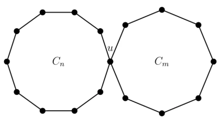
4.2.1 Join of two cycles . . . 43
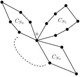
4.2.2 Join of several cycles . . . 47
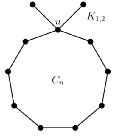
4.2.3 Join of a cycle and a claw . . . 52
4.2.4 Join of several paths . . . 55
5 Graph-transformations preserving periodicity 59
5.1 Multiplex graph . . . 59
5.2 Subdivision . . . 59
5.3 Line graphs induced by Hoffman graphs . . . 63
5.3.1 Hoffman graphs . . . 63
5.3.2 Definition of staggered walks . . . 66
5.3.3 Periodicity of staggered walks . . . 67
Chapter 1
Introduction
A quantum walk is interpreted as a quantum analogy of a random walk [23] and has been actively discussed in various fields such as quantum physics and computer sciences [47], [63] since Y. Aharonov et al. [2] introduced a quantum random walk as an antecedent of a quantum walk in 1993. The motivation was to detect a single atom in the excited state on some photons in a cavity as fast as possible. Slightly later, there has been an increasing interest in quantum walks on graphs in relation to searching problems [54], graph-isomorphism problems [15] and so forth. A quantum walk often shows a specific characteristic which is not observed in a random walk and the characteristic helps us to solve the problems. What we focus on in this paper is periodicity of quantum walks, which is one of the most important property of quantum walks [28], [41]. Especially, in order to shed light on the profound relation between quantum walks and graph structure we consider characterization of graphs which admit a periodic quantum walk. In this paper, we give not only an extended result of [28] but also a condition of structure to allow periodicity. Furthermore, we introduce some graph-transformations preserving the periodicity.
Unlike a random walk, a particle of a quantum walk has chirality and its motion is interpreted as a wave propagation on the underlying graphs [17]. More precisely, a particle has an amplitude expressed in terms of a Hilbert space associated to the underlying graph and the time evolution is given by a unitary operator. Then the quantum interference, that is, overlaps and cancellations of waves play an important role. Then the unitary time evolution ensures that the amplitude at each time always gives the probability distribution. There are two types of, quantum walks: discrete- and continuous-time quantum walks. Both types have been intensively studied with many applications. Indeed, one of the principal motivations to investigate quantum walks was to design quantum systems solving problems more efficiently than classical systems. As a strong evidence, Shor [59] provided a quantum algorithm to solve an integer factorization and a discrete logarithm problem, which gave an exponential speedup over classical algorithms. In addition, Grover [22] also provided a quantum search algorithm for an unordered database, which gives a quadratic speedup over classical search algorithms.
For discrete-time quantum walks, Meyer [49] proposed quantum cellular automata to realize a physical device for quantum computations. The cell automata gave foundation of
discrete-time quantum walks on the one-dimensional lattice. Nayak and Vishwanath [52] formulated a discrete-time quantum walk called the Hadamard walk on the one-dimensional lattice by taking the Shor¨odinger’s approach to obtain the asymptotic form of the probabil-ity distribution. Later, Ambainis et al. [4] analyzed quantum walks on the one-dimensional lattice not only by the Schr¨odinger’s approach but also using path integrals. After that, Konno [35], [36] reformulated quantum walks on the one-dimensional lattice and obtained the weak limit theorem for quantum walks corresponding to the central limit theorem for a random walk. Moreover, it was shown that the proper time scaling for a quantum walk to obtain a reasonable weak limit is linear in construct to a classical random walk of which the proper time scale is the square root of time. It is one of the reasons why quantum algorithms are more efficient than classical ones. Another widely studied topic on quan-tum walk is localization which means that the particle stays at an initial position at a high probability. The localization is found in the one-dimensional lattice [37], the half line [40] and so forth. Furthermore, coexistence of the linear spreading and the localization of a quantum walk is also mentioned in [27].
While discrete-time quantum walks on the one-dimensional lattice were intensively studied, quantum walks on general graphs were in the limelight as an extension of the one-dimensional lattice by several researchers. D. Aharonov et al. [3] first gave an idea of quantum walks on the general graphs, where a quantum version of the mixing time, the filling time and the dispersion time are defined. In particular, a quadratically fast conver-gence of the mixing time for quantum walks on cycles are mentioned and the lower bound of the mixing time is obtained for general graphs. Szegedy [62] defined a quantum walk on bipartite graphs and formulated the quantum hitting time. The quantum hitting time is proved to be quadratically faster than the classical one. Furthermore, Childs et al. [13] and Kempe [33] proposed exponentially faster quantum hitting times. As is seen in those works, quantum walks on graphs suggest to realize more efficient systems to solve several problems such as searching problems. Indeed, searching algorithms to detect a target set on graphs as fast as possible by driving a quantum walk have been intensively analyzed. Aaronson et al. [1] and Shenvi et al. [58] proposed quantum search algorithms to find a marked item on a d-dimensional lattice and the hypercube. These algorithms are shown to provide a quadratical speed up. As an application of quantum searchings, Ambainis [6] formulated an algorithm to solve element distinctness more efficiently. Moreover, Magniez
et al. [46] proposed a quantum algorithm to find triangles on a graph.
Continuous-time quantum walks are also well-studied fields, where the time evolution operator is defined by a Hamiltonian. Farhi [16] first proposed an idea of continuous-time quantum walks to solve a decision problem. It can be regarded as a quantum algorithm on a tree. A family of trees which provides an exponentially speedup to solve the problem than classical algorithms was found in the result. In particular, the perfect state transfer is one of the most interesting topics on continuous-time quantum walks. If there exist two vertices u, v such that the state of particle on u completely transfers to the another one
v, such a phenomenon is called perfect state transfer. Bose [10] first proposed the perfect
state transfer. Some classes of graphs which admit perfect state transfer were found in [8], [19], [34], and [61]. Furthermore, Godsil [19] found spectral restriction of graphs admitting
perfect state transfer. However, it is still open what kind of graph structure is required to provide the perfect state transfer.
What we deal with in this paper is characterization of graphs in terms of specific char-acteristics of quantum walks, or in short, relation between graph structure and quantum walks. In this context it is worthwhile to discuss periodicity of discrete-time quantum walks which one of the most significant characteristics of quantum walks. The periodicity in this paper means that there exists an integer k ∈ N such that the k-th power of the time evolution operator becomes the identity operator. Thus, for a periodic quantum walk, the behavior of the particle becomes periodic. Recently, the periodicity of discrete-time quantum walks has been studied in [28], [41], [43], [66] and [67]. The periodicity is an interesting property of quantum walks but it is very flail. The periodicity often disappears even if we give a small change to the graph. Therefore, we are interested in what kind of graph structure gives or preserves the periodicity. In addition, research on quantum walks pays attention to analyze properties of quantum walks for a fixed graph. On the contrary, we aim to characterize graph structure given by a property of quantum walks. This standpoint is regarded as an inverse problem from the viewpoint of quantum walks.
We mainly treat the periodicity of the Grover walk, which is a quantum walk derived from Grover’s search algorithm. The Grover walk is one of the most intensively studied quantum walks on graphs [5], [64]. A graph-isomorphism problem is one of the most interesting applications of the Grover walks. It is used to distinguish two cospectral strongly regular graphs in terms of the adjacency matrix. The cube of the time evolution operator of the Grover walk is believed to be an invariance of these graphs [15], [20]. Ren et al. [57] gave a relation between the Ihara zeta function and the Grover walk. Furthermore, Konno and Sato [39] expressed the characteristic polynomial of the time evolution operator of Grover walk in terms of the second weighted zeta function. It is remarkable that the spectrum of the time evolution operator of the Grover walk is reduced to that of the transition operator of a simple random walk on the underlying graph [27], [30], [48]. Such a spectral mapping is useful for some problems of quantum walks such as searching problems. Structural quantities of a graph such as the degree or the diameter are often retrieved from a simple random walk. If we suppose the periodicity of the Grover walk, there must be restriction to a simple random walk on the graph and the restriction inherits to the graph structure. Thus, we may see graph structure restricted by the periodicity. This is the principal reason why we choose the Grover walk.
This paper is organized as follows: As preliminaries, we give definition of graphs, graph-transformations, and associated operators in Chapter 2. In addition, we introduce the Chebyshev polynomials and their properties, which are useful tools throughout this paper. In Chapter 3, we define the Grover walk and its periodicity. Especially, the spectral expression of the time evolution operator appeared in Lemma 3.2.2 plays an important role in this paper. By spectral analysis, we give several classes of graphs on which a periodic Grover walk is exhibited, i.e., cycle graphs and path graphs, see Theorems 3.4.1 and 3.5.1, respectively. We next treat classes of graphs having an equitable partition, i.e., Hamming graphs, Johnson graphs, and generalized Bethe trees. The main results are stated in Theorems 3.6.3, 3.6.4, and 3.7.6. Indeed, these results give an extension of the
ones in [28].
In Chapter 4, we derive a condition of a graph to admit a periodic Grover walk in The-orem 4.1.2, which is the most important statement in this paper. Thereby, we construct new classes of graphs by an operator called join on which a periodic Grover walk is exhib-ited. We join two cycles, several cycles, a cycle and a claw, and several path graphs and show that the Grover walks on these graphs are periodic in Theorems 4.2.1, 4.2.2, 4.2.3, and 4.2.4, respectively. Moreover, we find the shape of graphs admitting an odd-periodic Grover walk in Theorem 4.3.1.
In Chapter 5, we introduce, as graph-transformations, multiplex graphs, subdivision graphs and generalized line graphs induced by a Hoffman graph. We show that multiplex and subdivision graph preserve the periodicity of Grover walks in Theorems 5.1.1, and 5.2.1, respectively. Furthermore, we study another quantum walk called staggered walk on a generalized line graph. Combining the ideas of multiplex and subdivision graphs, we show that the staggered walk on the generalized line graph becomes periodic whenever the Grover walk on the original graph is periodic, see Theorem 5.3.2.
Finally, Chapter 6 summarizes the main results. In addition, we discuss some future directions. We extend the condition of periodicity and state some works derived from the extended conditions.
Chapter 2
Preliminaries
In this Chapter, we prepare basic notions and notations of graphs, and introduce several classes of graphs and graph-transformations. Moreover, we recall the Chebyshev polyno-mials and their useful properties.
2.1
Graphs
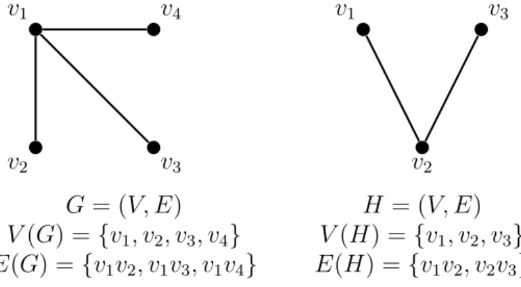
A graph G = (V, E) is composed of a vertex set V (G) and an edge set E(G). The vertex set V (G) is a countable set and an element of V (G) is called a vertex. The edge set E(G) is a 2-element subset of V (G) and an element of E(G) is called an edge. We say that two vertices u, v ∈ V (G) are adjacent (denoted by u ∼ v), if an unordered pair {u, v} is a member of E(G). An edge connecting u and v is denoted by uv and these vertices are called the endpoints of uv. Then
E(G) = {uv | u, v ∈ V (G), u ∼ v}.
We may relax the above conditions to allow a multiple edge. In that case E(G) is
under-v1 v2 v3 v4 G = (V, E) V (G) ={v1, v2, v3, v4} E(G) ={v1v2, v1v3, v1v4} v1 v2 v3 H = (V, E) V (H) = {v1, v2, v3} E(H) ={v1v2, v2v3}
stood as a multiset. Let muv be the multiplicity of an edge uv. Then we express the edge
set by
E(G) ={uv(muv)| u ∼ v}.
A graph having a multiedge is called a multigraph. For a multigraph G, we define a simple graph called the underlying graph G by
V (G) = V (G), E(G) ={uv | uv ∈ E(G)}.
In other words, the underlying graph is given by regarding a multiedge as a single edge.
v2 v1 v3 v4 G = (V, E) V (G) ={v1, v2, v3, v4} E(G) = {v1v2(2), v1v3(1), v1v4(3)} Figure 2.2: A multigraph
If a multigraph has no multiedge, it is called a simple graph. An edge uv ∈ E(G) may be given two directions, i.e., from u to v and from v to u. Then an edge with a direction is called an arc. We denote an arc from u to v by (u, v). For a simple graph G we define the symmetric arc set by
A(G) = {(u, v), (v, u) | uv ∈ E(G)}.
For a multigraph, the symmetric arc set is denoted by
A(G) = {(u, v; j), (v, u; j) | uv ∈ E(G), 1 ≤ j ≤ muv},
where muv is the multiplicity of an edge uv.
Let u ∈ V (G) and e ∈ E(G). If u is one of the endpoints of e, we write u ≈ e. If two edges e and f have a common endpoint, then we write e ≈ f. Let G and H be graphs. If H satisfies that V (H) ⊂ V (G) and E(H) ⊂ E(G), H is a subgraph of G by definition. Let S be a subset of V (G) and H a subgraph of G with V (H) = S. If each edge satisfying that both endpoints belong to S is in E(H), H is called the induced subgraph spanned by
S and is denoted by G[S]. For a vertex u ∈ V (G), every vertex v with v ∼ u is called a neighbor of u and we define
The number of neighbors of u is called the degree of u and denoted by degG(u). If there is no danger of confusion, omitting the subscripts we write deg(u). A vertex of degree one is called a leaf. A sequence of distinct vertices{u0, u1. . . , uk} ⊂ V (G) satisfying ui ∼ ui+1
for 0 ≤ i ≤ k − 1 is called a path from u0 to uk. If u0 ∼ uk in addition, the sequence
{u0, u1. . . , uk, u0} is called an essential cycle. We define the distance between u, v ∈ V (G)
to be the length of a shortest path from u to v and denote it by d(u, v).
Furthermore, if|V (G)| < ∞, the graph G is called finite. If there exists a path between any pair of vertices, the graph G is called connected. Throughout this paper, we only deal with finite and connected graphs. In that case, we define the diameter of G by
diam(G) := max
u,v∈V (G)d(u, v).
We will introduce several fundamental classes of graphs in the next subsection. In partic-ular, if the vertex set of G is decomposed into the disjoint union of two subsets such that any vertex in each subset is not adjacent each other, then G is called a bipartite graph. Thus, the lengths of all the essential cycles in G are even if and only if G is a bipartite graph. A graph G with unique essential cycle is called a unicycle graph. If the number of vertices of the unique essential cycle of a unicycle graph is odd (resp. even), then the graph is called an odd-unicycle graph (resp. even-unicycle graph). If the degrees of all the vertices of G are constant, then G is called a regular graph. If the degree of a regular graph is k, it is called a k-regular graph. Moreover, a graph G having no essential cycle is called a tree.
2.1.1
Several classes of graphs
Here, let us introduce several important classes of graphs.
• Cycle graphs.
For n∈ N with n ≥ 3, the cycle graph on n vertices is denoted by Cn. For V (Cn) =
{v1, . . . , vn}, the edge set E(Cn) is defined by
E(Cn) ={vivi+1 | 1 ≤ i ≤ n},
where we tacitly understand that vn+1 = v1.
• Path graphs.
For n∈ N, the path graph on n vertices is denoted by Pn. For V (Pn) = {v1, . . . , vn},
the edge set E(Pn) is defined by
Figure 2.3: A cycle graph
Figure 2.4: A path graph
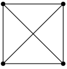
• Complete graphs.
For n ∈ N, the complete graph on n vertices is denoted by Kn. For V (Kn) =
{v1, . . . , vn}, the edge set E(Kn) is defined by
E(Kn) = {vivj | 1 ≤ i < j ≤ n}.
Then all the vertices are adjacent each other. Let G be a graph and S be a subset of V (G). If G[S] becomes a complete graph, S is called a clique.
Figure 2.5: A complete graph
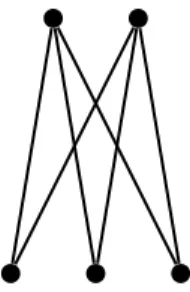
• Complete bipartite graphs.
For r and s ∈ N, the complete bipartite graph, denoted by Kr,s, is defined as a
bipartite graph with two disjoint subsets A and B with |A| = r, |B| = s such that
E(Kr,s) = {uv | u ∈ A, v ∈ B}.
Then any vertex in A is adjacent to every vertex in B. For r ≥ 2, the graph K1,r is
Figure 2.6: A complete bipartite graph
• Strongly regular graphs.
For n, k, λ, µ ∈ N a strongly regular graph SRG(n, k, λ, µ) is defined as a k-regular graph on n vertices such that
|N(u) ∩ N(v)| = λ
if u∼ v and
|N(u) ∩ N(v)| = µ
otherwise.
Figure 2.7: A strongly regular graph SRG(10, 3, 0, 1)
2.1.2
Graph-transformations
Let G and G′ be families of graphs. Then mappings from G to G′ are called
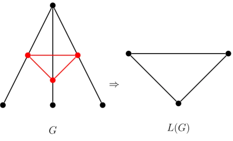
Graph-transformations. We introduce useful graph-Graph-transformations. • Line graph.
G
⇒
L(G)
Figure 2.8: A line graph
For a simple graph G the line graph L(G) is defined by
V (L(G)) := E(G),
E(L(G)) :={e, f ∈ E(G), ef | e ≈ f and e ̸= f}.
In other words, each edge in G is regarded as a vertex of L(G) and two vertices of L(G) are adjacent if and only if their corresponding edges in G has a common neighbor.
• Multiplex graph.
For n ∈ N, a multigraph given by replacing each edge of G by a multiedge with multiplicity n is called the multiplex graph M Pn(G) in this paper. To be precise,
M Pn(G) is defined by
V (M Pn(G)) := V (G),
E(M Pn(G)) :={e(n) | e ∈ E(G)}.
• Subdivision graph.
Set V (G) = {vi | 1 ≤ i ≤ n}. For l ∈ N, the l-subdivision graph Sl(G) is given by
embedding the path graph with length l in each edge of G. For e = vivj ∈ E(G), let
us denote the path graph embedded to e by P(e). We define
V (P(e)) :={w(r)i,j | 0 ≤ r ≤ l}, and
G
⇒
M P3(G)
Figure 2.9: A multiplex graph
where we tacitly understand that wi,j(0) = vi, w
(l) i,j = vj and w (r) i,j = w (l−r) j,i for 0≤ r ≤ l. Then we have V (Sl(G)) = V (G)∪ ⊔ e∈E(G) V (P(e)) and E(Sl(G)) = ∪ e∈E(G) E(P(e)).
In other words, Sl(G) is given by adding l− 1 vertices to each edge of G.
G
⇒
S4(G)
2.1.3
Operators associated to graphs
For a countable set Λ, we define the Hilbert space of square summable functions on Λ by
ℓ2(Λ) :={f : Λ → C | ∥f∥2 <∞},
where the inner product and the norm are given by
⟨f, g⟩ :=∑
x∈Λ
f (x)g(x)
and
∥f∥ :=√⟨f, f⟩,
respectively. The standard basis of ℓ2(Λ) is given by {δ
x | x ∈ Λ}, where δx(y) = 1 if
x = y and δx(y) = 0 otherwise. Let us define the identity operator on ℓ2(Λ) by IΛ, that is,
IΛf = f for any f ∈ ℓ2(Λ). For a finite Λ, let jΛ and 0Λ be the all-one and zero function in
ℓ2(Λ), respectively. That is, j
Λ(x) = 1, 0Λ(x) = 0 for any x∈ Λ. Throughout this paper,
for an operator X on ℓ2(Λ) we denote the set of eigenvalues of X by σ(X).The support of
f ∈ ℓ2(Λ) is defined by
supp(f ) :={x ∈ Λ | f(x) ̸= 0}.
For a simple graph G = (V, E), we define the adjacency operator A = A(G) as follows:
Af (u) =∑
v∼u
f (v), f ∈ ℓ2(V (G)).
Define the transition operator T = T (G) by
T f (u) = 1
deg(u) ∑
v∼u
f (v), f ∈ ℓ2(V (G)),
and the degree operator M = M (G) by
M f (u) = deg(u)f (u), f ∈ ℓ2(V (G)).
Then it follows immediately that
T = M−1A.
Then the representation matrices of A and T with respect to the standard basis {δu | u ∈
V (G)} are written as Au,v = { 1, if u∼ v, 0, otherwise, and Tu,v = { 1 deg(u), if u∼ v, 0, otherwise.
We sometimes consider the symmetric transition operator ˜ T = M12T M− 1 2 = M− 1 2AM− 1 2
instead of T since their spectra are in coincidence. If G is a multigraph, the transition operator is defined as follows:
T f (u) =∑
v∼u
muv
Mu
f (v), f ∈ ℓ2(V (G)), (2.1)
where muv is the multiplicity of an edge uv and Mu =
∑
v∼umuv. The transition operator
expresses a random walk on G. If G is simple, it expresses a simple random walk on G. In that case, it is easily shown that jV (G) is an eigenfunction of T for 1, which is the maximum
eigenvalue. Thus, 1∈ σ(T ) and the absolute values of all the eigenvalues of T is at most one. It is known that −1 ∈ σ(T ) if G is a bipartite graph [12].
2.2
Chebyshev polynomials
Let{Tj}∞j=0 and {Uj}∞j=0 be sequences of polynomials satisfying
T0(λ) = 1, T1(λ) = λ,
U0(λ) = 1, U1(λ) = 2λ
and the same recurrence relation;
Lj(λ) = 2λLj−1(λ)− Lj−2(λ), j ≥ 2.
Then{Tj(λ)} and {Uj(λ)} are called the Chebyshev polynomials of the first and of the
sec-ond kind, respectively. For the Chebyshev polynomials of the secsec-ond kind, it is convenient to set U−1(λ) = 0. The coefficients of the term of the maximum degree of Tj(λ) and Uj(λ)
become 2j−1 and 2j, respectively. From the above relations, it follows that
Tj(cos θ) = cos(jθ),
Uj(cos θ) =
sin((j + 1)θ) sin θ ,
for j ∈ N and θ ∈ R. We will provide some key properties of the Chebyshev polynomials.
Lemma 2.2.1. If a complex sequence {ai}∞i=0 satisfies
λai =
1
2(ai−1+ ai+1)
for λ∈ C, then we have
Proof. Straightforward by induction.
Lemma 2.2.2. Let j ≥ 0 and λ ∈ C. (i) λUj(λ)− Uj−1(λ) = Tj+1(λ).
(ii) λTj(λ)− Tj−1(λ) = (λ2− 1)Uj−1(λ).
(iii) U2
j(λ)− Uj−1(λ)Uj+1(λ) = 1.
Chapter 3
Periodicity of Grover walks
In this Chapter, we define the Grover walk and touch its periodicity which is our main topic in this paper. Preparing some useful tools to analyze the periodicity, we characterize several classes of graphs which admit periodic Grover walks.
3.1
Grover walks
Let G be a multigraph. Here, a particle moves around arcs of the underlying graph rather than vertices. In addition, the motion of the particle can be interpreted as a dynamics on the arcs. Now, we give a unitary operator on ℓ2(A(G)) defined by
U φ(f ) = ∑ o(f )=t(e) ( 2 deg(t(f )) − δe,f−1 ) φ(e), φ∈ ℓ2(A(G)),
where δe,f is the Kronecker delta symbol. Then U is called the Grover transfer operator
and the quantum walk defined by the above U is called the Grover walk. Let φ0 ∈ ℓ2(A(G))
be a function with ∑
e∈A(G)
|φ0(e)|2 = 1.
Then we define a sequence {φt}∞t=0 as
φt = Utφ0. (3.1)
Due to the unitarity of U , we have ∑
e∈A(G)
|φt(e)|2 = 1
at each time t. Thus, we understand that the value |φt(e)|2 is the finding probability of
the particle on e at time t. Now, the equation (3.1) gives the dynamics of the Grover walk. Then the function φt and the value φt(e) are called the quantum state and amplitude,
3.2
Periodic Grover walk
Let G be a multigraph and U the Grover transfer operator. If there exists a positive integer
k ∈ N such that Uk = IA(G), the Grover walk on G is periodic. In that case, the smallest
k ∈ N such that Uk= I
A(G) is called the period of the Grover walk. For simplicity, we call
a graph satisfying the above condition a Grover-periodic graph. Especially, if the period is specified as k, we call the graph a Grover-k-periodic graph.
Proposition 3.2.1. A graph G is Grover-k-periodic if and only if λk = 1 for every λ ∈
σ(U ) and there exists λ∈ σ(U) such that λj ̸= 1 for 0 < j < k. Proof. Immediate by diagonalization of U .
Let U be the Grover transfer operator with σ(U ) ={λ1, λ2, . . . , λd}. We set
Ni := min{k ∈ N | λki = 1, 1≤ i ≤ d.}
Then the period of the Grover walk is given by
N = lcm(N1,N2, . . . ,Nd),
where the right-side stands for the least common multiple of N1,N2, . . . ,Nd.
Lemma 3.2.2 (Higuchi, Konno, Sato, Segawa [28]). Let G be a multigraph. The spectrum
of the Grover transfer operator U is given by
σ(U ) ={e±i cos−1(σ(T (G)))} ∪ {1}b1(G)∪ {−1}b1(G)−1+1B(G) ,
where b1(G) =|E(G)| − |V (G)| + 1 and 1B(G) = 1 if G is bipartite, 1B(G) = 0 otherwise.
Throughout this paper, the branch of cos−1 is specified as [0, π]. If G is simple, b1(G)
coincides with the number of the essential cycles in G, and called the first Betti number.
Proposition 3.2.3. A graph G is Grover-periodic if and only if every eigenvalue of T is
the real part of a root of unity, that is,
cos−1(σ(T (G)))⊂ πQ.
Proof. By Proposition 3.2.1, every eigenvalue of U is the root of unity if G is
Grover-periodic. Hence, it holds cos−1(σ(T (G)))⊂ πQ by Lemma 3.2.2.
Let us define the Joukowski transformation J : C\{0} → C as follows: For z ∈ C,
J (z) := z + z−1
Lemma 3.2.4. For z ∈ C with |z| = 1 and j ≥ 0 the following relations hold: (i) (2z)jT j(J (z)) = 2j−1(z2j + 1). (ii) (2z)jUj(J (z)) = 2j i ∑ k=0 z2j−2k,
where Tj and Uj are the Chebyshev polynomials of the first and second kind, respectively.
Proof. Straightforward by direct calculation.
Lemma 3.2.5 (Higuchi, Konno, Sato, Segawa [28]). Let f be a monic and rational
poly-nomial of degree n. Then the zeros of f are the real parts of a root of unity if and only if the polynomial (2z)nf (J (z)) is a product of some cyclotomic polynomials for z ∈ C with |z| = 1.
Proof. Let λ1, λ2, . . . , λd be the distinct zeros of f , that is,
f (x) =
d
∏
k=1
(x− λk)mk,
where mk is the multiplicity of λk. Suppose that they are the real parts of a root of unity.
Then we have (2z)nf (J (z)) = (2z)n d ∏ k=1 ( z + z−1 2 − λk )mk = d ∏ k=1 (z2− 2λkz + 1)mk = d ∏ k=1 {(z − eiθk)(z− e−iθk)}mk, (3.3)
where θk = cos−1(λk). Since θk ∈ πQ and f is rational, the right-hand side of (3.3) is a
product of cyclotomic polynomials.
3.3
Related works
Finite graphs that admit periodic quantum walks have been investigated. It is shown [41] that the Hadamard walk on the cycle Cn is periodic if and only if n = 2, 4 or 8, whose
periods are 2, 8, or 24, respectively. In [28], periodic Szegedy walks on finite graphs are analyzed. The Szegedy walk is induced from a random walk on the underlying graph and the Grover walk is a special case of the Szegedy walk induced from a simple random walk. In [28], Szegedy walks induced from not only a simple random walk but also from a lazy random walk are considered. The results are summarized as follows:
• Complete graphs.
The Szegedy walk on a complete graph Kn with n≥ 2 induced from a lazy random
walk with a laziness l is periodic if and only if (n, l) = (2, 0), (3, 0),(n,n1),(2,14)and (
n,n+12n ), whose periods are 2, 3, 4, 6 and 6, respectively.
• Complete bipartite graphs.
The Szegedy walk on a complete bipartite graph Kr,s with r + s≥ 3 induced from a
lazy random walk with a laziness l is periodic if and only if l = 0 or 12, whose periods are 4 or 12, respectively.
• Strongly regular graphs.
The Szegedy walk on a strongly regular graph SRG(n, k, λ, µ) induced from a simple random walk is periodic if and only if
(n, k, λ, µ) = (5, 2, 0, 1), (2k, k, 0, k), (3λ, 2λ, λ, 2λ),
whose periods are 5, 4, or 12, respectively. Those graphs are nothing but C5, Kk,k,
and Kλ,λ,λ, respectively.
• Cycle graphs.
Here, we consider the cycle graph Cn (n ≥ 3), and set C2 = P2. For V (Cn) =
{v1, v2, . . . , vn} with v1 = vn+1, define the transition probability from vi to vi+1 and
from vi+1 to vi for 1 ≤ i ≤ n by p and 1 − p with p ̸= 12, respectively. Then the
Szegedy walk on a cycle graph Cn induced from the non-reversible random walk with
the above transition probabilities is periodic if and only if
(i) n = 2 and p = 2−4√3,2−4√2 or 14, whose periods are 6, 8 or 12, respectively.
(ii) n = 4 and p = 2−4√3,2−4√2 or 14, whose periods are 12, 8 or 12, respectively.
(iii) n = 8 and p = 2−√2
4 whose period is 24.
3.4
Cycle graphs
Theorem 3.4.1. The cycle graph Cn is Grover-periodic for any n ≥ 3, and its period is
n.
Proof. Let A = A(Cn) and T = T (Cn) be the adjacency and transition operators,
respec-tively. It is well-known (e.g., [12]) that
σ(A) = { 2 cos2π n j | 0 ≤ j ≤ n − 1 } .
Since Cn is a 2-regular graph, it follows immediately that
T = 1
and σ(T ) = { cos2π n j | 0 ≤ j ≤ n − 1 } .
Thus, it follows that cos−1(σ(T )) ⊂ πQ. By Proposition 3.2.3, we assert that the graph
Cn is Grover-periodic and its period is n for n∈ N.
3.5
Path graphs
Theorem 3.5.1. The path graph Pn is Grover-periodic for any n ≥ 2, and its period is
2(n− 1).
Proof. Set G = Pn and let T = T (G) be the transition operator. Suppose that λf = T f
for f ∈ ℓ2(V (G)), that is,
λf (u) = 1 deg(u) ∑ v∼u f (v), u∈ V (G). Then we have λf (v1) = f (v2), (3.4) λf (vn) = f (vn−1), (3.5) λf (vi) = 1 2(f (vi−1) + f (vi+1)), 2≤ i ≤ n − 1 (3.6) From (3.6) we see that
f (vi+1) = 2λf (vi)− f(vi−1), 2≤ i ≤ n − 1.
In view of Lemma 2.2.1, we obtain
f (vi+1) = Ui−1(λ)f (v2)− Ui−2(λ)f (v1),
where{Ui(λ)} is the Chebyshev polynomial of the second kind. By (3.4) and (i) of Lemma
2.2.2, we have
f (vi+1) = λUi−1(λ)− Ui−2(λ)f (v1)
= Ti(λ)f (v1), (3.7)
where{Ti(λ)} is the Chebyshev polynomial of the first kind. In particular, setting i = n−1,
we get
f (vn) = Tn−1(λ)f (v1).
On the other hand, taking (3.5) into account, we have
λTn−1(λ) = λf (vn)
= f (vn−1)
If f (v1) = 0, we see from (3.7) that f (v) = 0 for v∈ V (G), which is not an eigenfunction.
Hence, f (v1)̸= 0 and we obtain
λTn−1(λ)− Tn−2(λ) = 0
(λ2 − 1)Un−2(λ) = 0,
where we applied (ii) of Lemma 2.2.2 to the first equation. We set λ = cos θ for 0 < θ < π. Then Un−2(λ) = 0 if and only if
sin (n− 1)θ sin θ = 0, from which we obtain
λ = cos π
n− 1j, 0 < j < n− 1.
Thus, we find n− 2 distinct eigenvalues together with linearly independent eigenfunctions of T . The remaining eigenvalues are±1 since G is a bipartite graph. Since 2 + (n − 2) = n coincides with |V (G)|, we obtain
σ(T ) = { cos π n− 1j | 0 < j < n − 1 } ∪ {±1}.
Obviously, cos−1(σ(T )) ⊂ πQ, which implies that G is Grover-periodic and its period is 2(n− 1) by Proposition 3.2.3.
3.6
Distance-regular graphs
Let G = (V, E) be a simple graph. If V (G) is decomposed into a disjoint union of non-empty subsets Γ1, Γ2, . . . , Γr ⊂ V (G), then π = {Γ1, Γ2, . . . Γr} is called a partition of G. If
Γi is a clique for 1 ≤ i ≤ r, we call π a clique partition. A partition π is called an equitable
partition, if there exists a non-negative integer bi,j such that each vertex u ∈ Γi has bi,j
neighbors in Γj for every pair of indices i, j, regardless the choice of u, that is,
|N(u) ∩ Γj| = bi,j
for 1≤ i, j ≤ r and u ∈ Γi.
3.6.1
Definition of distance-regular graphs
Let G be a simple, k-regular graph. Let d = diam(G). For a vertex x∈ V (G), we define Γj(x) := {y ∈ V (G) | d(x, y) = j}, 0 ≤ j ≤ d. (3.8)
Then G is a distance-regular graph if it holds that
|N(y) ∩ Γj−1(x)| = cj, (3.9)
|N(y) ∩ Γj(x)| = aj, (3.10)
|N(y) ∩ Γj+1(x)| = bj, (3.11)
for any x ∈ V (G), 1 ≤ j ≤ d and y ∈ Γj(x). Then {Γ0(x), Γ1(x),· · · , Γd(x)} becomes
an equitable partition of G. The above non-negative parameters {aj, bj, cj} are called the
intersection numbers [11]. In addition, it holds that for 0≤ j ≤ d,
cj + aj+ bj = k, (3.12)
where we set c0 = bd = 0. From the connectivity of G it follows immediately that bi ̸=
0, cj ̸= 0 for 0 ≤ i ≤ d − 1 and 1 ≤ j ≤ d.
3.6.2
Restriction on diameter
For an operator X, let us denote the number of distinct eigenvalues of X is denoted by
n(X). For any graph G and its adjacency operator A = A(G), it is well-known that
diam(G) < n(A) [12]. This relation also holds for the transition operator, that is,
diam(G) < n(T ), (3.13)
which is proved in a similar way.
Theorem 3.6.1. Let r be a rational number with|r| ≤ 1. Then it holds that cos−1(r)∈ πQ
if and only if r∈ { 0,±1, ±1 2 } .
Proof. We only show the necessity since the sufficiency is clear. Put h(x) = x− r. Then
we have
2z· h (J (z)) = z2− 2rz + 1. (3.14) By Lemma 3.2.5 and Theorem 3.6.1, (3.14) is a product of cyclotomic polynomials. Ac-cording as r = 0,±1, or ±12, (3.14) becomes
z2+ 1,
z2± 2z + 1, z2± z + 1,
which are products of cyclotomic polynomials.
Theorem 3.6.2. Let G be a Grover-periodic graph. If all the eigenvalues of T (G) are
rational, it holds necessarily that
diam(G) < 5.
Proof. Let λ be an eigenvalue of T (G). By Proposition 3.2.3, we have λ ∈ {0,±1, ±12}. Then it follows n(T )≤ 5. In view of (3.13), we obtain diam(G) < 5.
3.6.3
Hamming graphs
For positive integers d ≥ 1 and q ≥ 2 the Hamming graph H(d, q) is defined as follows: Let F be a finite set of q elements. The vertex set of H(d, q) is Fd and two vertices
x = (x1, x2,· · · , xd), y = (y1, y2,· · · , yd)∈ Fd are adjacent if |{i | xi ̸= yi, 1 ≤ i ≤ d}| = 1.
It follows that the graph is d(q − 1)-regular and diam(H(d, q)) = d. Let A and T be the adjacency and transition operators of H(d, q), respectively. It is known [11] that the distinct eigenvalues of the adjacency operator A are given by
σ(A) ={d(q − 1) − qi | 0 ≤ i ≤ d}.
Then it follows immediately that
σ(T ) = { 1− qi d(q− 1) 0 ≤ i ≤ d } .
Theorem 3.6.3. The only Grover-periodic Hamming graphs H(d, q) are
H(1, 2), H(1, 3), H(2, 2), H(3, 3), H(4, 2) whose periods are 2, 3, 12, and 12, respectively.
Proof. For d = 1, the Hamming graph is nothing but else the complete graph Kq. It is
known [28] that the complete graph Kq is Grover-periodic if and only if q = 2 or 3. Then
the Grover-periodic Hamming graphs H(1, q) are the cases of q = 2 and 3, whose periods are 2 and 3, respectively. Now, we suppose d ≥ 2 and every eigenvalue of T is rational. From the proof of Theorems 3.6.1 and 3.6.2, it follows that diam(H(d, q)) = d < 5 and
σ(T )⊂ { 0,±1, ±1 2 } . (3.15) For d = 2, we have σ(T ) = { 1− 2q 2(q− 1), 1− q 2(q− 1), 1 } .
Then it is easily seen that q = 2 only fulfills (3.15) and we have
σ(T ) ={−1, 0, 1}.
Thus, we have d = q = 2. The only Grover-periodic Hamming graph among H(2, q) is
H(2, 2)≃ C4 and the period is 4. For d = 3 we have
σ(T ) = { 1− q q− 1, 1− 2q 3(q− 1), 1− q 3(q− 1), 1 } .
Then q = 3 only fulfills (3.15) and we have
σ(T ) = { −1 2, 0, 1 2, 1 } .
Thus, the only Grover-periodic Hamming graph among H(3, q) is H(3, 3) and the period is 12. For d = 4, we have σ(T ) = { 1− q q− 1, 1− 3q 4(q− 1), 1− q 2(q− 1), 1− q 4(q− 1), 1 } .
Similarly, we obtain q = 2 and
σ(T ) = { −1, −1 2, 0, 1 2, 1 } .
Thus, the only Grover-periodic Hamming graph among H(4, q) is H(4, 2), and the period is 12.
3.6.4
Johnson graphs
For two positive integers n and k with n ≥ k, the Johnson graph J(n, k) is defined as follows: The vertices of J (n, k) are the k-element subsets of a fixed n-element set. Two vertices X, Y ∈ V (J(n, k)) are adjacent if |X ∩ Y | = k − 1. It follows that the graph is
k(n− k)-regular and diam(J(n, k)) = min{k, n − k}. Let A and T be the adjacency and
transition operators of J (n, k), respectively. It is known that the d + 1 distinct eigenvalues of A are given by
σ(A) ={(d − j)(n − d − j) − j | 0 ≤ i ≤ d},
where d = min{k, n − k} [11]. Hence, we obtain
σ(T ) = { (d− j)(n − d − j) − j d(n− d) | 0 ≤ j ≤ d } .
Theorem 3.6.4. The only Grover-periodic Johnson graphs J (n, k) are
J (2, 1), J (3, 1), J (4, 2) whose periods are 2, 3 and 12, respectively.
Proof. Note that every eigenvalue of the transition operator of J (n, k) is rational. Hence,
we have d < 5 by Theorem 3.6.2. For d = 1, we have
σ(T ) = { − 1 n− 1, 1 } .
In order to achieve (3.15), it necessarily holds that n = 2 or 3. If d = k, that is, 2k ≤ n, then we obtain (n, k) = (2, 1) and (3, 1). If d = n− k, that is, 2k ≥ n, then we obtain (n, k) = (2, 1) and (3, 2). Indeed, it is easily checked that J (3, 2) ≃ J(3, 1). Thus the Grover-periodic Johnson graphs J (n, 1) are J (2, 1) or J (3, 1), which are nothing but else
K2 or K3, respectively. For d = 2 we have
σ(T ) = { − 1 n− 2, n− 4 2n− 4, 1 } .
Hence, it is necessary that n = 3 or 4. If n = 3, we have k = 2 or 1 according as the diameter is d = k or d = n−k. However, these pairs satisfy neither the assumption 2k ≤ n for d = k nor 2k ≥ n for d = n − k. If n = 4, we obtain k = 2 for both of the cases d = k and d = n− k and we have
σ(T ) = { −1 2, 0, 1 } .
Thus, the graph is J (4, 2) and the period is 12. For the cases of d = 3 and d = 4, we obtain
σ(T ) = { − 1 n− 3, n− 7 3n− 9, 2n− 9 3n− 9, 1 } and σ(T ) = { − 1 n− 4, n− 10 4n− 16, 2n− 14 4n− 16, 3n− 16 4n− 16, 1 } ,
respectively. However, any n does not fulfill (3.15) for both of the two cases. Thus, there are no Grover-periodic Johnson graphs for d = 3 and d = 4.
3.7
Generalized Bethe trees
3.7.1
Definition
Let G be a tree and fix an arbitrary x∈ V (G). For j ≥ 0, let Γj(x) be defined as in (3.8)
and n be defined as Γn(x)̸= ϕ and Γn+1(x) = ϕ. The rooted tree G is called a generalized
Bethe tree if
|N(u) ∩ Γi+1(x)| = d(i), 0 ≤ i ≤ n − 1,
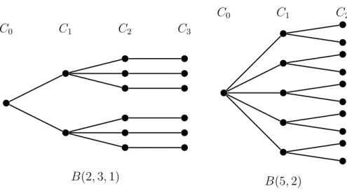
is independent of u∈ Γi. In that case, the graph is denoted by B(d(0), d(1), . . . , d(n− 1)).
Note that {Γ0(x), Γ1(x), . . . , Γn(x)} becomes an equitable partition of G. For simplicity,
we put Ci := Γi(x). Examples of generalized Bethe trees are shown in Figure 3.1. For
u ∈ Ci with i ̸= 0, n, the child and parent of u are defined to be vertices in N(u) ∩ Ci+1
and N (u)∩ Ci−1, respectively.
C0 C1 C2 C3
B(2, 3, 1)
C0 C1 C2
B(5, 2)
Figure 3.1: Examples of generalized Bethe trees Define D0 = 1 d(1) + 1, Di = d(i) (d(i) + 1)(d(i + 1) + 1), 1≤ i ≤ n. For 0 ≤ i ≤ n let us define
Ψi = 1 √ Ci ∑ v∈Ci δv
and let A be the subspace of ℓ2(V (G)) spanned by Ψ
0, Ψ1, . . . , Ψn. Then it follows that
A⊥= { f ∈ ℓ2(V (G)) ∑ v∈Ci f (v) = 0, 0 ≤ i ≤ n } .
It is easily checked that T is invariant on A⊥. By direct calculation, the following holds.
Lemma 3.7.1. For a generalized Bethe tree B(d(0), d(1),· · · , d(n − 1)), it holds that
˜ T Ψi = √ D0Ψ1, i = 0, √ Dn−1Ψn−1, i = n, √ DiΨi+1+ √ Di−1Ψi−1, otherwise.
The representation matrix of ˜T with respect to {Ψ0, Ψ1,· · · Ψn} becomes
˜ T|A = 0 √D0 √ D0 0 √ D1 √ D1 0 √ D2 . .. . .. . .. √ Dn−2 0 √ Dn−1 √ Dn−1 0 .
3.7.2
Spectral analysis of transition operator
Let G = B(d(0), d(1),· · · , d(n − 1)) be a generalized Bethe tree. For v ∈ V (G)\C0 let
P (v) be the parent of v. For 1≤ i ≤ n − 1 we define Pi(v) = P (P (· · · P (P
| {z }
i
(v))),
and set P0(v) = v. For v ∈ V , we define N
n(v)⊂ V (G) by
Nn(v) ={w ∈ Cn|∃j, Pj(w) = v}.
We define a sequence of polynomials in λ∈ C inductively as follows: g0(λ) = 1, g1(λ) = λ, gi(λ) = (d(n− i + 1) + 1) λgi−1(λ)− d(n − i + 1)gi−2(λ), 2≤ i ≤ n, gn+1(λ) = d(0)(λgn(λ)− gn−1(λ)).
Then it is easily checked that the coefficient of the maximum degree of gi is i−1 ∏ j=1 (d(n− j) + 1), 2 ≤ i ≤ n, and that of gn+1 is d(0) ∏n−1 j=1(d(n− j) − 1).
Moreover, let us define
Ω :={1 ≤ i ≤ n | d(n − i) ≥ 2}. For i∈ Ω and v∗ ∈ Cn−i, let N (v∗)∪ Cn−i+1 ={v1, v2, . . . , vl}.
Lemma 3.7.2. For every i∈ Ω the zeros of gi are eigenvalues of T . Let λ be a zero of gi.
Then the following function f ∈ ℓ2(V (G)) is an eigenfunction of T for λ and f ∈ A⊥.
For w ∈ Nn(v1), 0≤ j ≤ i − 1, f (Pj(w)) = gj(λ); for w∈ Nn(v2), 0≤ j ≤ i − 1, f (Pj(w)) =−gj(λ); for w∈ Cn\ (Nn(v1)∪ Nn(v2)), 0≤ j ≤ i − 1, f (Pj(w)) = 0; for w∈ ∪nj=0−iCj, f (w) = 0.
Proof. For any u∈ ∪nj=0−iCj\{v∗} it holds clearly that (T f)(u) = λf(u). For v∗, we have
(T f )(v∗) = 1 deg(v∗) ∑ x∼v∗ f (x) = 1 deg(v∗)(f (v1) + f (v2)) = 1 deg(v∗)(gi−1(λ)− gi−1(λ)) = 0 = λf (v∗).
For any w ∈ Nn(v1) and 0≤ j ≤ i − 1 it follows that (T f )(Pj(w)) = 1 deg(Pj(w)) ∑ u∼Pj(w) f (u) = 1 d(n− j) + 1 f(Pj+1(w)) + ∑ u∼Pj(w) u∈Cn−j+1 f (u) = 1 d(n− j) + 1(gj+1(λ) + d(n− j)gj−1(λ)) = λgj(λ) = λf (Pj(w)).
For any w ∈ Nn(v2) and every 0≤ j ≤ i − 1 it similarly holds that
(T f )(Pj(w)) =−λgj(λ) = λf (Pj(w)).
Furthermore, it is clear that
(T f )(Pj(w)) = 0 = λf (Pj(w))
for any w ∈ Cn\ (Nn(v1)∪ Nn(v2)) and 0 ≤ j ≤ i − 1. Thus, (T f)(x) = λf(x) for
x∈ ∪nj=n−i+1Cj. Hence, it holds that (T f )(x) = λf (x) for any x∈ V (G).
Since ∑u∈C
if (u) = 0 for any 0 ≤ i ≤ n by the definition of f, we have f ∈ A
⊥.
It follows from Lemma 3.7.2 that σ( ˜T|A⊥)⊃∪i∈Ω{λ ∈ C | gi(λ) = 0}.
Lemma 3.7.3. It holds that
σ( ˜T|A⊥) =
∪
i∈Ω
{λ ∈ C | gi(λ) = 0}.
Proof. For the assertion it is sufficient to show that the number of the linearly independent
eigenfunctions obtained during the above argument coincides with dimA⊥=|V (G)|−(n+ 1). By definition of a generalized Bethe tree it follows that |C0| = 1 and
|Ci| = i−1 ∏ j=0 d(j), 1≤ i ≤ n − 1. (3.16) Thus, |V (G)| = n ∑ i=0 |Ci| = |C0| + n−1 ∑ i=0 |Cn−i| = 1 + n−1 ∑ i=0 n−i−1∏ j=0 d(j).
Then it holds that dimA⊥ = ∑ni=0−1∏nj=0−i−1d(j) − n. For i ∈ Ω, let λ be a zero of gi.
By Lemma 3.7.2 there are d(n− i) − 1 linearly independent eigenfunctions for λ for every
v ∈ Cn−i. Hence, we find |Cn−i| (d(n − i) − 1) linearly independent eigenfunctions for λ.
The zeros of giare the eigenvalues of a diagonal matrix and all the eigenvalues of the
tri-diagonal matrices are simple [53]. Hence, the number of the linearly independent eigenfunc-tions for to the zeros of giis i|Cn−i| (d(n − i) − 1). Here, we put Fi := i|Cn−i| (d(n − i) − 1)
for 1≤ i ≤ n. By (3.16) it follows that
Fi = i (n−i ∏ j=0 d(j)− n−i−1∏ j=0 d(j) ) ,
for 1 ≤ i ≤ n − 1 and Fn = n(d(0)− 1). Then the number of the linearly independent
eigenfunctions for the zeros of every gi for i ∈ Ω is
∑n
i=1Fi because Fi = 0 for i with
d(n− i) = 1. Thus, we get n ∑ i=1 Fi = n−1 ∑ i=1 i (n−i ∏ j=0 d(j)− n−i−1∏ j=0 d(j) ) + Fn = n−1 ∑ i=1 ( i n−i ∏ j=0 d(j)− i n−i−1∏ j=0 d(j) ) + Fn = n−1 ∑ i=1 n−i ∏ j=0 d(j)− (n − 1)d(0) + n(d(0) − 1) = n−1 ∑ i=1 n−i ∏ j=0 d(j) + d(0)− n = n ∑ i=1 n−i ∏ j=0 d(j)− n,
which equals dimA⊥.
Here, let us put ˜g0(λ) = 1 and
˜ g0 = 1, g˜i = 1 ∏i−1 j=1(d(n− j) + 1) gi, 1≤ i ≤ n − 1. We define { p0(λ) = 1, pi(λ) = det(λIi− ˜T(i)), 1≤ i ≤ n + 1, (3.17)
where Ii is the i× i identity matrix and ˜T(i) is the principal submatrix of ˜T|A given by
removing the first row up to the (n+1−i)-th row and the first column up to the (n+1−i)-th column.
Lemma 3.7.4. It holds that
pi(λ) = ˜gi(λ)
for any λ∈ C and 0 ≤ i ≤ n + 1.
Proof. Since ˜g0(λ) = p0(λ) = 1 and ˜g1(λ) = p1(λ) = λ, it is sufficient to show that {˜gi}
and {pi} satisfy the same recurrence relation. First, by the cofactor expansion, we have
pi(λ) = λpi−1(λ)− Dn−i+1pi−2(λ) (3.18)
for 0 ≤ i ≤ n + 1. If i = 2 or 3, it is easily seen that ˜gi(λ) = λ˜gi−1(λ)− Dn−i+1g˜i−2(λ)
since d(n) = 0. For 4≤ i ≤ n, ˜ gi(λ) = (d(n− i + 1) + 1)λgi−1(λ) ∏i−1 j=1(d(n− j) + 1) − d(n− i + 1)gi−2(λ) ∏i−1 j=1(d(n− j) + 1) = ∏i−2λgi−1(λ) j=1(d(n− j) + 1) − d(n− i + 1)gi−2(λ) (d(n− i + 1) + 1)(d(n − i + 2) + 1)∏ij=1−3(d(n− j) + 1) = λ˜gi−1(λ)− Dn−i+1g˜i−2(λ).
We have ˜gn+1(λ) = λ˜gn(λ)− D0g˜n−1(λ) since gn+1(λ) = d(0)(λgn(λ)− gn−1(λ)) and D0 = 1
d(1)+1, so we see that pi(λ) = ˜gi(λ) for any λ∈ C and 0 ≤ i ≤ n + 1.
Then it follows immediately that the zeros of pn+1(λ) are the eigenvalues of ˜T|A.
In-deed, the polynomials {pi}ni=0 are the monic orthogonal polynomials with Jacobi
coeffi-cients {√D0,
√
D1,· · · ,
√
Dn−1}. Then together with Lemma 3.7.3, the above discussion
is summarized as follows:
Theorem 3.7.5. It holds that
σ( ˜T|A⊥) =
∪
i∈Ω
{λ ∈ C | pi(λ) = 0},
σ( ˜T|A) ={λ ∈ C | pn+1(λ) = 0}.
3.7.3
Grover-periodic generalized Bethe trees
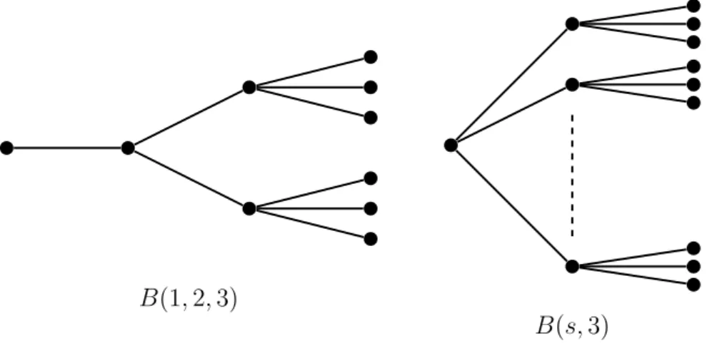
Theorem 3.7.6. The only Grover-periodic generalized Bethe trees are Sk(B(1, 2, 3)) and
B(1, 2, 3)
B(s, 3)
Figure 3.2: Grover-periodic generalized Bethe trees
Proof. Let G = B(d(0), d(1),· · · , d(n)) be a generalized Bethe tree and put l = |Ω|. We
define positive integers k1, k2, . . . , kl in such a way that n− Ki ∈ Ω for 1 ≤ i ≤ l, where
Ki =
∑i
j=1kj (See Figure 3.3). Then we define kl+1 = n− Kl and Kl+1 = kl+1+ Kl = n.
Moreover, we put di = d(n− Ki). By Lemmas 3.7.4 and 3.7.2, the zeros of pKi are the
eigenvalue of ˜T|A⊥ for 1 ≤ i ≤ l, and those of pK(l+1)+1 are the eigenvalues of ˜T|A. We
will find the polynomial pKi and check whether (2z)
Kip
Ki(J (z)) is a product of cyclotomic
polynomials for every 1≤ i ≤ l + 1. The argument will be divided into a few steps.
C0 kl+1 z }| { Cn−Kl pKl Cn−K2 k2 z }| { pK2 Cn−K1 k1 z }| { pK1 C0 Figure 3.3: Setting
Lemma 3.7.7. Let pi be defined as in (3.17). For 1 ≤ i ≤ K1, it holds that
pi =
1
Proof. If K1 = 1, 2, then it clearly holds because p1 = λ = T1, and p2 = λp1 − Dn−1p0 =
λ2 − 1 2 =
1
2T2. Here, we assume that K1 ≥ 3. We prove it by induction on i. Indeed,
Dn−i+1 = 14 for 3≤ i ≤ K1 and it holds that
pi = λpi−1− Dn−i+1pi−2 = λ { 1 2i−2Ti−1 } − 1 4 { 1 2i−3Ti−2 } = 1 2i−1 (2λTi−1− Ti−2) = 1 2i−1Ti.
Lemma 3.7.8. For 2≤ j ≤ l + 1 with kj ≥ 2 and 2 ≤ i ≤ kj, it holds that
pK(j−1)+i =
1
2i−2Ui−2pK(j−1)+2−
1
2i−1Ui−3pK(j−1)+1. (3.20)
Proof. It is easy to confirm that (3.7.8) holds for i = 2 and 3. Then we assume that i≥ 4
and we have pK(j−1)+i = λpK(j−1)+i−1− Dn−K(j−1)−i+1pK(j−1)+i−2 = λpK(j−1)+i−1− 1 4pK(j−1)+i−2 = λ { 1 2i−3Ui−3pK(j−1)+2− 1 2i−2Ui−4pK(j−1)+1 } − 1 4 { 1 2i−4Ui−4pK(j−1)+2− 1 2i−3Ui−5pK(j−1)+1 } = 1 2i−2(2λUi−3− Ui−4)pK(j−1)+2− 1 2i−1(2λUi−4− Ui−5)pK(j−1)+1 = 1 2i−2Ui−2pK(j−1)+2− 1 2i−1Ui−3pK(j−1)+1.
If l = 0, the graph is nothing but else the path graph Pn+1, which is the
Grover-2n-periodic graph. If l = 1, the graph is expressed as
B(1, 1,| {z }· · · , 1
k2
, d1, 1, 1,| {z }· · · , 1
k1−1
).
If k2 = 0 and k1 = 1, or k2 = 1 and k1 = 1, then these graphs are nothing but else claws,
which are Grover-4-periodic graphs. Hence, we omit these cases. By Lemma 3.7.7, we have
pK1 =
1
Furthermore, it follows by (i) on Lemma 3.2.4 that (2z)K1p
K1(J (z)) = z
2K1 + 1, (3.21)
which is a cyclotomic polynomial. The zeros of (3.21) are the eigenvalues of ˜T|A⊥ and
satisfy
z4k1 = 1. (3.22)
These are 4k1-th roots of unity. Next, we find the polynomial pn+1 = pK2+1 to analyze the
eigenvalues of ˜T|A. Then we have
pK1+1 = { λp1− dd1 1+1p0 if k1 = 1, λpK1 − d1 2(d1+1)pK1−1 if k1 ≥ 2, and pK1+2 = { λpK1+1− 1 d1+1pK1 if k2 = 1, λpK1+1− 1 2(d1+1)pK1 if k2 ≥ 2.
Indeed, for any k1 ∈ N, we have
(2z)K1+1p K1+1(J (z)) = z 2K1+2+ 1− d1 d1+ 1 z2K1 + 1− d1 d1+ 1 z2 + 1. (3.23) Furthermore, if k2 = 1, then (2z)K1+2p K1+2(J (z)) = z 2K1+4− 2 d1+ 1 z2K1+2+ 1− d1 d1+ 1 z2K1 + 1− d1 d1+ 1 z4 − 2 d1 + 1 z2+ 1 (3.24) and if k2 ≥ 2, then (2z)K1+2p K1+2(J (z)) = z 2K1+4+1− d1 d1+ 1 z2K1 +1− d1 d1+ 1 z4+ 1 (3.25) by (i) on Lemma 3.2.4. If k2 = 1, then K2 + 1 = K1 + 2. Furthermore, if k2 = 2, then
K2+ 1 = K1+ 3, i.e., pK2+1 = pK1+3= λpK2+2−
1
2pK1+1. Therefore, it follows that pK2+1 = pK1+2 if k2 = 1, λpK1+2− 1 2pK1+1 if k2 = 2, 1 2k2−2(λUk2−2− Uk2−3) pK1+2− 1 2k2−1 (λUk2−3− Uk2−4) pK1+1. if k2 ≥ 3,
by Lemma 3.7.8. Using (3.23), (3.24), (3.25) and (ii) on Lemma 3.2.4, we get (2z)K2+1p K2+1(J (z)) = z 2K2+2− z2K2 +1− d1 d1 + 1 ( z2k2+2− z2k2 − z2K1+2+ z2K1)− z2+ 1.
Unless k1 = K1 = k2, the above polynomial is not an integer polynomial, which implies
that it is not a product of cyclotomic polynomials. Thus, the Bethe tree is nothing k1
-subdivision of Sk2(K1,d1+1). Then the above polynomial becomes z4k1+2− z4k1 − z2+ 1 = (z2− 1)(z4k1 − 1)
and the zeros satisfy z4k1 = 1. Therefore, the period is 4k
Lemma 3.7.9. If G is Grover-periodic and l ≥ 2, it holds that k1 = k2 and d1 = 3.
Proof. By Lemma 3.7.8, we obtain
pK2 = { pK1+1 if k2 = 1, 1 2k2−2Uk2−2pK1+2− 1 2k2−1Uk2−3pK1+1 if k2 ≥ 2.
Indeed, for any k1, k2 ∈ N it follows that
(2z)K2p K2(J (z)) = z 2K2 +1− d1 d1+ 1 z2k1 +1− d1 d1+ 1 z2k2 + 1 (3.26)
by (3.23), (3.24), (3.25), and (ii) of Lemma 3.2.4. Thus, (3.26) is not an integer polynomial unless k1 = k2 and d1 = 3.
Then (3.26) turns to
z4k1 − z2k1 + 1, (3.27)
and the zeros satisfy
z12k1 = 1. (3.28)
Lemma 3.7.10. If l≥ 3, then G is not Grover-periodic.
Proof. We suppose l ≥ 3 and derive a contradiction. Then the zeros of pK3 are the
eigenvalue of ˜T on A⊥ by Theorem 3.7.5. Then we also have
pK3 = { pK2+1 if k3 = 1, 1 2k3−2Uk3−2pK2+2− 1 2k3−1Uk3−3pK2+1 if k3 ≥ 2.
by Lemma 3.7.8. We set k1 = k2, and d1 = 3 from Lemma 3.7.9. Therefore, it follows that
K2 = 2k1 and pK2+2 = λpK2+1− 1 2(d2+ 1) pK2 pK2+1 = { λpK2 − d2 4(d2+1)pK2−1 if k1 = k2 = 1, λpK2 − d2 2(d2+1)pK2−1 if k1 = k2 ≥ 2. pK2−1 = pK1 if k1 = k2 = 1, pK1+1 if k1 = k2 = 2, 1 2k1−3Uk1−3pK1+2− 1 2k1−2Uk1−4pK1+1 if k1 = k2 ≥ 3.
Combining (3.21), (3.23), (3.24), (3.25), and (3.27), we have
(2z)K2−1p K2−1(J (z)) = z 4k1−2− 1 2z 2k1 − 1 2z 2k1−2+ 1, (3.29)
(2z)K2+1p K2+1(J (z)) = z 4k1+2+1− d2 d2+ 1 z4k1 − 1 d2 + 1 z2k1+2− 1 d2+ 1 z2k1 +1− d2 d2+ 1 z2+ 1, (3.30) (2z)K2+2p K2+2(J (z)) = z 4k1+4+1− d2 d2+ 1 z4k1 − 1 d2 + 1 z2k1+4− 1 d2+ 1 z2k1 +1− d2 d2+ 1 z4+ 1. (3.31) Thus, for any k1, k3 ∈ N we have
(2z)K3p K3(J (z)) = z 2K3+1− d2 d2+ 1 z4k1− 1 d2+ 1 z2k1− 1 d2+ 1 z2k1+2k3+1− d2 d2+ 1 z2k3+1. (3.32)
The above polynomial is not an integer polynomial for any d2 ∈ N≥2, and k1, k3 ∈ N. In
other words, the zeros of pK3 are not roots of the real part of the unity for any d2 ∈ N≥2,
and k1, k3 ∈ N. Therefore, we have to set l < 3 so that the zeros of pK3(λ) are not the
eigenvalues of ˜T .
Therefore, the candidates of Grover-periodic generalized Bethe trees are written as
B(1, 1,· · · , 1 | {z } k3 , d2, 1, 1,| {z }· · · , 1 k1−1 , 3, 1, 1,· · · , 1 | {z } k1−1 ), (3.33) or, B(d2, 1, 1,| {z }· · · , 1 k1−1 , 3, 1, 1,| {z }· · · , 1 k1−1 ). (3.34)
For (3.33), we consider the eigenvalues of T|A to determine the parameters k3 ∈ N
and d2 ∈ N≥2. We find pn+1 = pK3+1 and analyze its zeros since these coincide with the
eigenvalues of ˜T|A. Then we have
pK3+1 = { λpK3 − 1 d2+1pK2 if k3 = 1, λpK3 − 1 2pK3−1 if k3 ≥ 2.
For k1, k3 ∈ N the polynomials (2z)K3pK3(J (z)) and (2z)
K2p
K2(J (z)) are of the forms
(3.32) and (3.27), respectively. By (3.27), (3.30), (3.31) and
pK3−1 = pK2 if k3 = 1, pK2+1 if k3 = 2, 1 2k3−3Uk3−3pK2+2− 1 2k3−2Uk3−4pK2+1 if k3 ≥ 3, we have (2z)K3−1p K3−1(J (z)) = z 2(K3−1)+ 1− d2 d2+ 1 z4k1− 1 d2+ 1 z2k1 − 1 d2+ 1 z2k1+2(k3−1)+ 1− d2 d2+ 1 z2(k3−1)+ 1. (3.35)